Article

A Parametric Study of Trailing Edge Flap Implementation on Three Different Airfoils Through an Artificial Neuronal Network

by
Igor Rodriguez-Eguia
1,
Iñigo Errasti
2,
Unai Fernandez-Gamiz
2,*,
Jesús María Blanco
1,
Ekaitz Zulueta
3 and
Aitor Saenz-Aguirre
4
1
Department of Nuclear Engineering and Fluid Mechanics, University of the Basque Country (UPV/EHU), Plaza Ingeniero, Torres Quevedo 1, 48013 Bilbao, Spain
2
Department of Nuclear Engineering and Fluid Mechanics, University of the Basque Country (UPV/EHU), Nieves Cano, 12, 01006 Vitoria-Gasteiz, Spain
3
Department of System Engineering and Automation Control, University of the Basque Country (UPV/EHU), Nieves Cano, 12, 01006 Vitoria-Gasteiz, Spain
4
Department of Nuclear Engineering and Fluid Mechanics, University of the Basque Country (UPV/EHU), Avenida Otaola, 29, 20600 Eibar, Spain
*
Author to whom correspondence should be addressed.
Symmetry 2020, 12(5), 828; https://doi.org/10.3390/sym12050828
Submission received: 22 April 2020 / Revised: 7 May 2020 / Accepted: 9 May 2020 / Published: 18 May 2020
(This article belongs to the Special Issue Aero/Hydrodynamics and Symmetry 2020)

Abstract

:
Trailing edge flaps (TEFs) are high-lift devices that generate changes in the lift and drag coefficients of an airfoil. A large number of 2D simulations are performed in this study, in order to measure these changes in aerodynamic coefficients and to analyze them for a given Reynolds number. Three different airfoils, namely NACA 0012, NACA 64(3)-618, and S810, are studied in relation to three combinations of the following parameters: angle of attack, flap angle (deflection), and flaplength. Results are in concordance with the aerodynamic results expected when studying a TEF on an airfoil, showing the effect exerted by the three parameters on both aerodynamic coefficients lift and drag. Depending on whether the airfoil flap is deployed on either the pressure zone or the suction zone, the lift-to-drag ratio, CL/CD, will increase or decrease, respectively. Besides, the use of a larger flap length will increase the higher values and decrease the lower values of the CL/CD ratio. In addition, an artificial neural network (ANN) based prediction model for aerodynamic forces was built through the results obtained from the research.

Graphical Abstract

1. Introduction

Wind turbine sizes have steadily been increasing over the past few years. Commercial offshore wind turbines with a maximum capacity of up to 6 MW are operational in the U.S., Europe, and China. Indeed, 10 MW turbines with diameters of 144 m and even 20 MW turbines with diameters of 240 m are currently under development, as Musial et al. [1] and Fichaux [2] et al. have reported. Barlas et al. [3] stated that one main focus is on developing new technologies capable of considerably reducing ultimate and fatigue loads in wind turbines. If an innovative blade design can result in a decrease in loading, Veers et al. [4] concluded in their study that the general cost will decrease, as rotor loads affect the loading of other components, such as the drive train and the tower.
According to the study of Yu et al. [5], two load control methods are widely used for commercial offshore wind turbines: collective pitch control and relatively advanced individual pitch control. Although they can alleviate rotor loads, several limitations and problems still exist [4]. More advanced, fast, and precise local aerodynamic controls are urgently needed to circumvent such limitations. With that end in sight, the concept of a smart rotor control was presented in [6,7].
As Fernandez-Gamiz et al. [8,9] explained, the idea is to use control devices that locally change the aerodynamic performance of the airfoil on the wind turbine blade.
That innovation in combination with appropriate sensors measuring the aerodynamic forces and a controller, which processes the sensor signals and generates an actuation signal, is defined as the ‘smart’ rotor concept.
Van Wingerden et al. [10] suggested that the aerodynamic forces can be minimized with properly designed actuators, sensors, and controllers. Van Dam et al. [11] compiled some of the most important techniques that could be used in wind turbines to assure the safest and the most favorable operation under different atmospheric conditions. According to Yagiz et al. [12], active and passive flow control techniques are used for drag and lift optimization in air-vehicles.
Wood [13] developed a four-layer scheme that can be used to classify the different concepts that are part of all flow control devices. Aramendia et al. [14] classified them as active or passive, depending on their operating principle. Passive control techniques would present an improvement in the turbine efficiency and aerodynamic forces reduction without external energy consumption. Active control techniques need an additional energy source to generate the desired effect on the flow.
A study by Houghton and Bell [15] claimed that the yearly 9% increase in installed wind energy in Europe over the past fifteen years shows the significance of research in the field of flow control for large wind turbines. According to Joncas et al. [16] and Buhl et al. [17], some research on this topic has been performed in the wind industry, where the trailing edge flap (TEF) has been used for load alleviation. More recently, Barlas et al. [18] provided a detailed summary of research into smart rotor control for wind turbines and concluded that the deformable trailing edge flap (DTEF) was the most efficient aerodynamic control method in contrast to other potential candidates, such as microtabs, morphing, active twist, and suction/blowing strategies, synthetic jets, active vortex generators, etc.
The device of interest in this study is the TEF. These foils were first developed, according to Abbot et al. [19], to improve the lift coefficient (CL) of airplane wings and to increase lift force during take-off and landing without changing the characteristics of cruising and high-speed flight. They are categorized by Abdelrahman and Johnson [20] as high-lift devices, which also include leading edge slats, slotted-flaps, and external airfoil flaps.
TEFs can be classified into two different groups [11]: traditional and non-traditional trailing-edge flaps. The traditional flaps are the most frequently used. As Aramendia et al. [14,
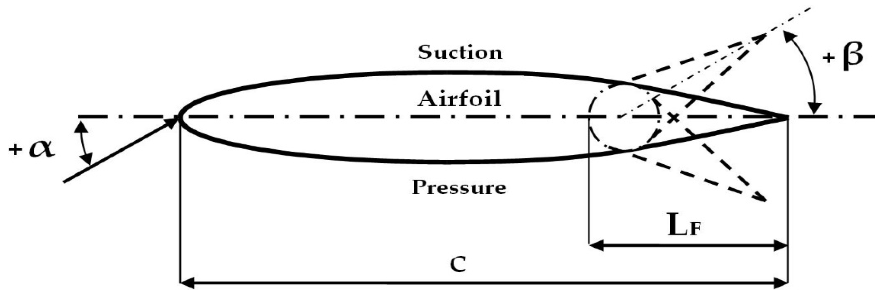
21] explained, their main concept is based on the increase (deployment on the pressure side) or decrease (deployment on the suction side) of the airfoil camber. The camber line, which measures the curvature of the airfoil, will generate more lift in the airfoil as its curvature is greater. So, if the flap is deployed on the pressure side, the lift increases, and if the flap is deployed on the suction side, the lift decreases.
TEFs can be employed in two ways: discrete flaps require a moment on the hinge to achieve the required position, while flexible flaps present a smoother shape between the device and the airfoil, which increases their efficiency. The scheme of a trailing edge flap installed on an airfoil is shown in Figure 1.
Non-traditional TEFs operate on the same principle as traditional ones, but they use newer technology such as piezoelectrics and ‘smart’ materials. Quickly activated, they are lightweight, and occupy a shorter chord to improve load alleviation. However, scalability to large models and the durability and reliability of the deployment devices can be inherent drawbacks [11].
Johnson et al. [22] commented on the three most relevant non-traditional TEFs: The compact TEF (see Roth et al. [23]), the adaptive compliant wing (see Kota et al. [24]), and the adaptive trailing edge geometry [10,17].
Lackner M. et al. [25] presented the benefits of using flow control devices such as TEFs. Basualdo [26] showed that the use of variable geometry airfoils in wind turbine blades can lead to load alleviation. Andersen et al. [27] report the potential of flaps to alleviate 34% of the fatigue equivalent damage in flapwise loading, while Barlas et al. [28] find slightly lower values up to 27%. The success of the static angle testing of the modular blade flaps and the ability of the system to measure moment changes within the blade introduces numerous possibilities for further research [20].
A parametric study of trailing edge flap implementation on three different airfoils through an artificial neuronal network is presented in this article.
There are two main contributions made by this study: On the one hand the high number of simulations and different parameters combinations performed for three different airfoils, on the other hand, the use of an artificial neural network.
As shown in the methodology section, the large number of simulations performed is due to the high number of specifically designed combinations that have been carried out between different parameters (flap angle β and flaplength LF). In addition, as it has also been specified in the same section, this research increases the analysis ratio of some parameters with respect to the state of the art.
For different angles of attack, the relationship between aerodynamic forces, flap position and flaplength has been presented for each airfoil using an original three-dimensional surface. This research, apart from adding new knowledge about the effects of TEFs applied to three airfoils sections, has compared the results corresponding to the different airfoils in each step.
An artificial neural network-based prediction model for aerodynamic forces built through the results obtained from the research is presented in this study. The relevance of this type of mathematical solutions for control tools has been increased for the last decade.
Finally, in order to consolidate the results of this study, these are complemented with data on the near wake region and pressure.

2. Aims and Methodology

Aiming to optimize airfoil aerodynamic performance, the purpose of this study is a numerical assessment of the aerodynamic characteristics of airfoil sections, specifically intended for wind turbine applications, equipped with TEFs. For this, a parametric study of three different airfoils, NACA 0012, NACA 64(3)-618, and S810, with TEFs installed has been carried out. Then, with the aim of facilitate future computational control tools for TEFs and aerodynamic predictions tools, all the results have been used to build a mathematical prediction model through an artificial neural network which is more detailed in Section 4.4.
The airfoils used, are part of two different airfoil families. On the one hand, those corresponding to the National Advisory Committee of Aeronautics (NACA) airfoils, NACA 0012 and NACA 64 (3)-618, and on the other hand a wind turbine airfoil from the National Renewable Energy Laboratory (NREL), S810. Figure 2 illustrates precisely the outline of the three aerodynamic profiles:
The well-documented airfoil from the 4-digit series of NACA airfoils, the NACA 0012 is symmetrical; the 00 indicates that it has not camber. The 12 indicates that the airfoil has a 12% thickness to chord length ratio: it is 12% as thick as it is long. The main reason why this airfoil has been chosen together with the other two airfoils for this study is due to its symmetry. This symmetry helps the effects produced by the TEFs to be understood and shown more clearly. Recent studies carried out by Di et al. [29] and Al Mutairi et al. [30] show that NACA 0012 airfoil is still of interest of to the scientific community.
The NACA 64(3)-618 however, belongs to the “6 series” of the NACA family. 6 denotes the series and indicates that this group is designed for greater laminar flow than the 4-digit series. The second digit, 4, is the location of the minimum pressure in tenths of chord (0.4c). The number in parentheses 3 indicates that low drag is maintained at lift coefficients 0.3 above and below the design lift coefficient (0.6) specified by the first digit after the dash in tenths. The final two digits specify the thickness in percentage of chord, 18% (see [31]).
The S810 is a 18% thick, laminar-flow airfoil, designed specifically for HAWT applications (see Sommers [32]).
In order to measure aerodynamic coefficients, and later, analyze them, a large number of 2D simulations are performed in this study.
TEFs actuate at different angles as flow control devices on airfoil sections and are capable of changing their aerodynamic characteristics significantly. As Menon et al. [33] explained, the increase or decrease in lift depends on the relative angle between airfoil and flap sections (actuation angle, β) and the angle of relative wind (angle of attack, α).
This study, apart from the effect of the angles α and β, will also analyze the effect of different flaplengths (LF) in the change of lift.
The three different airfoils NACA 0012, NACA 64(3)-618, and S810 have five flaplengths of 8%, 9%, 10%, 12%, and 14% of the airfoil chord c that are combined with eleven flap angles from β = −5° to β = 5°, in one degree steps, yielding a total of 55 meshes. The simulations were performed for seventeen angles of attack from α = −6° to α = 10°, and in one-degree steps.
Procedure sketch showing the different combinations between flaplength, flap angle, and angle of attack, is shown in Figure 3.
Therefore, for each airfoil, a total number of 935 2D simulations were performed as a function of the angle of attack, the flap angle, and the flaplength.
In the course of the European UPWIND project at the Institute of Aerodynamics and Gas Dynamics (IAG), Lutz et al. [34], analyzed an airfoil specifically designed for load alleviation purposes equipped with 10% of c trailing edge flap. Moreover, as proposed by Wei Jun Zhu [35], the trailing edge flaps accounts for approximately 10% of the airfoil chord length. With the purpose of adding new insight of the effect of different flaplengths in the change of the lift and drag, this study chose a range of different flap lengths close to the 10% of c.
The cases studied by Menon et al. [33] in a similar research, involved three different angles of actuation of the flap: −5°, 0° and 5°. However, this study pretends to extend the previous study analyzing all the β angles between -5° and 5°, in one degree steps, so that the mapping charts shown later in the results section are supported by a greater number of points and are, therefore, of a higher quality.
The range of α angles (−6° till to +10° in one degree steps) used for the simulations of this study has been the necessary and sufficient to obtain the minimum and maximum values of the lift-to-drag ratio CL/CD, experiencing minimum and maximum figures respectively for these limits, as will be seen later in the results section.
According to Ju et al. [36], a high lift-to-drag ratio and a high lift coefficient are one of the principal aerodynamic requirements that a wind turbine airfoil should satisfy. So, this study has focused on the maximum CL/CD values, while stall regions will be studied in a following paper.
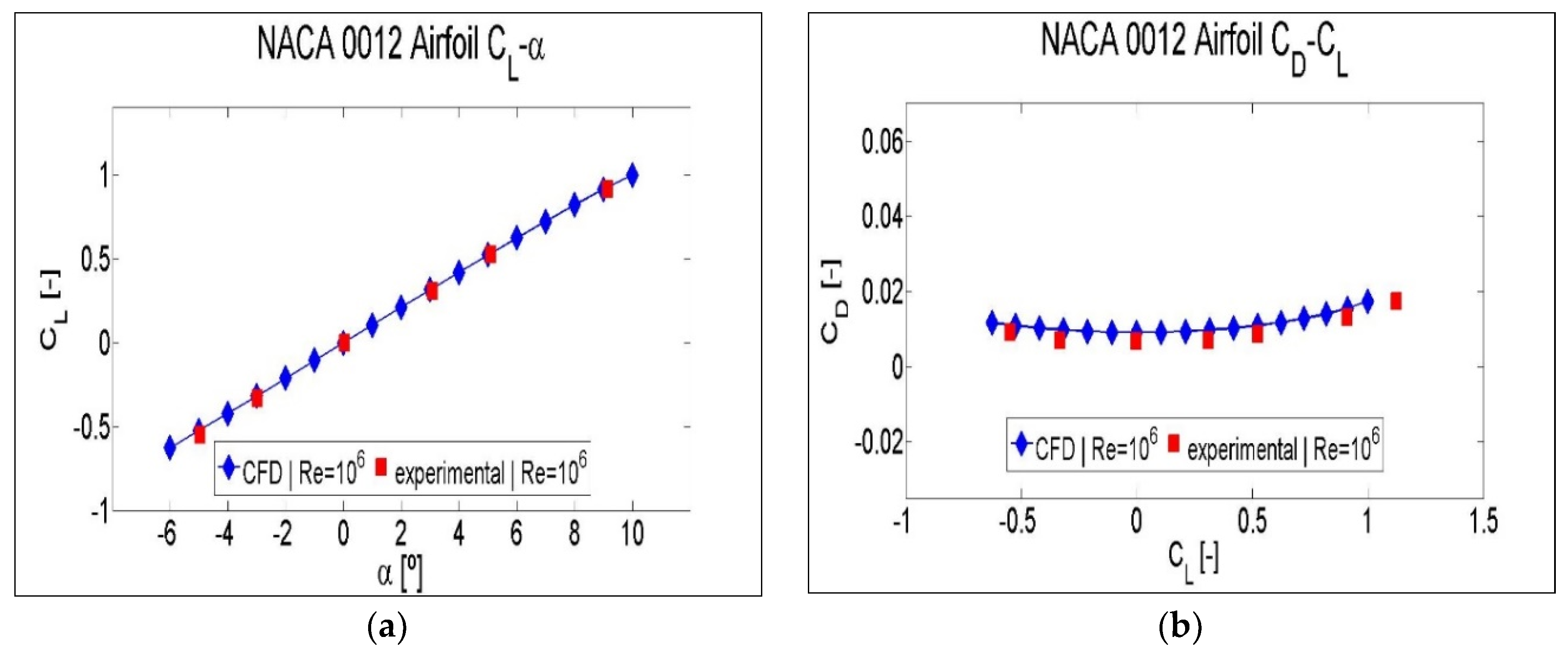
Computational simulations of the NACA 0012, the NACA 64(3)-618, and the S810 airfoils without a TEF were performed and validated against the experimental data provided by Douvi and Margaris [37], Abbot [19], and Reuss Ramsay et al. [38], respectively. These experimental data were obtained under similar boundary conditions to those of this study.

3. Numerical Setup

3.1. Computational Configuration and Procedure

CFD techniques have been employed, in order to obtain the aerodynamic features of the trailing edge flap (TEF) on an airfoil. Nowadays, non-commercial and proprietary CFD codes are used to reproduce most physical problems relatively well. In this work, the open source code OpenFOAM [39] was used to simulate the effects of different airfoil chords, depending on the TEF length with different flap angle positions installed on three different airfoils: NACA 0012, NACA 64(3)-618, and S810.
The potentialFoam solver which solves potential flow problems was used to generate starting fields, in order to speed up the convergence process. This solver is a suitable tool to generate the initial conditions for more advanced solvers, such as simpleFoam, the one used in the present work. The simpleFoam solver has been applied for steady-state, incompressible and turbulent flows using the RANS (Reynolds averaged Navier-Stokes) equations. Throughout the calculations, this solver uses the k-ω SST (shear stress transport) turbulence model developed by Menter [40], due to its robust performance in detached flows, as reported by Kral [41] and Gatski [42]. The turbulence model is a combination of two models: Wilcox’s k-ω model for near wall regions and the k-ε model for the outer region and in free shear flows. Second-order discretization schemes were employed in the computational simulations.
Python code was used for the generation of an optimized O-grid 2D mesh with a finite sharp trailing edge around the different types of airfoil under analysis. The coordinate points defining the airfoils, some from the airfoil coordinates database [43] and from Timmer et al. [44], were interpolated, in order to improve the surrounding mesh quality. The computational domain generated, shown in Figure 4, was a function of the O-grid radius, the flap angle and length, the airfoil geometry and the corresponding parameters such as chord and maximum thickness.
The cell number in the chord-wise direction was around 382 and in the normal direction 400. The outer boundary, according to the criteria followed by some authors [45], can be 40 chords away from the airfoil.
For this study, the patches of particular interest are inlet (inflow), outlet (zero gradient), and wall (airfoil).
The wall condition is a non-slip condition, constant zero velocity and no gradient pressure. The variables of particular interest which require boundary conditions (BC) are the fluid quantities velocity and pressure. The side patches of the domain have been defined as slip conditions.
For the current computations, the turbulence intensity has been set to 5%, and the mixing length has been estimated as a quarter of the airfoil chord length.
After having performed a sensitivity analysis, the number of cells of the O-grid 2D mesh was around 120,000. The python code output was fully compatible with the OpenFOAM blockMesh mesh utility, and the structured meshes were generated with proper stretching functions, yielding low expansion rates and dimensionless wall distance (y+ ≈ 1) for the Reynolds number under consideration.
Figure 5 shows the mesh around the trailing edge flap for its two extreme deployment positions, installed on one of the airfoils in this study. Each position of the TEF requires the generation of a new mesh for each airfoil. As proposed in Wei Jun Zhu [35], the trailing flap is designed as a flexible part which bends its sides when it flaps. Fincham et al. [46] used a similar concept in their study. However, in our particular model shown in Figure 1, for simplification, the flap shape is not modified, it is considered as a rigid body. The sub-chord length trailing flap rotates an angle β as a rigid body for each case with similar merging conditions for all the flap installation angles β, as a positive direction of the flap motion is considered counter clockwise rotation.
The orthogonality and skewness of the mesh of the three airfoils have been studied for the three airfoils and for three flap angles β. We chose the extreme values β = −5 and +5 degrees and the one with β = 0 degrees. The Table 1 summarizes the results of both mesh quality parameters.
A general rule is that the maximum skewness for a mesh in most flows should be kept below 0.95, which is the case in the present study as the maximum skewness is 0.87, for the NACA 64(3)-618 case (see Table 1):
As Belamadi et al. [47] used in a similar and recent research, the simulations considered a Reynolds number of Re = 106. The resulting flow speed is 15.11 m s−1. The Reynolds number is defined in Equation (1):
Re = ρ   U c μ   [ - ]
where ρ is the density, μ the absolute viscosity, c the reference length, which in the case of an airfoil is the chord length, and U the free stream velocity. Their values are shown in Table 2.
The Reynolds number is known, so the high (y) that the first row of grid cells should have is y = 3.65 × 10⁻⁵ m. Figure 6 shows the wall y+ distribution over the NACA0012 airfoil for two flap angle configurations β = 5° and −5°, angle of attack of α = 0° and flaplength of 8% of c.
In addition, the wall y+ parameter of the computations of the three airfoils have also been studied for two flap angle configurations β = 5° and β = −5°. Table 3 summarizes the results obtained in all cases for the non-dimensional wall y+ parameter. Angle of attack with α = 0° and flaplength of 8% of c.
Simulations were performed on a personal server-clustered parallel machine with Intel® Core i7-6700 CPU 3.40 GHz × 8 cores and 32 GB RAM on 64 bits Linux. Each domain corresponding to an O-grid mesh was automatically divided into eight subdomains to be solved in parallel, thereby reducing the simulation time.
The CD on the airfoil has been calculated by the application of Equation (2) in the far field planes normal to the flow direction and applied to the streamwise velocity in different wake rakes (WR), according to Beans et al. [48] and Young [49].
C D = 2 A   2 π   + u U   ( 1 u U ) y   dy   [ - ]
where A is the area determined by the chord length and the span, A = b × c. In our cases, 2D simulations have been carried out, and the drag coefficient CD has been calculated per meter of airfoil span.
The lift coefficient CL was determined by the OpenFOAM inbuilt code, which determines the value by means of the Equation (3):
C L = F L 1 2 ρ AU   [ - ]

3.2. Validation

The validations are represented in two different types of plots for each airfoil: (a) coefficient of lift against angle of attack CL–α; and, (b) drag coefficient to lift coefficient CD-CL in Figure 7, Figure 8 and Figure 9. Each pair of plots for each airfoil is represented by a different figure.
Figure 7a corresponds to the validation performed for the symmetric airfoil NACA 0012. The CL–α curves show that the lift CFD data at a Reynolds number of Re = 106 are coincident with the experimental ones [37]. Figure 7b, corresponding to the representation of the CD-CL curves, shows an over estimation of the drag CFD data with respect to the experimental ones. In order to highlight the trend of CFD data more clearly, the volume of CFD data used for the validation of the NACA 0012 airfoil is higher than the volume of the experimental points.
In the case of the NACA 64(3)-618 airfoil, the CFD data were obtained at a Reynolds number of Re = 106, but the experimental ones [19] were obtained at a Reynolds number of Re = 3 × 10⁶. This difference might explain an additional deviation in CD-CL curves. Therefore, Figure 8b shows that the CFD data for the drag are overestimated with respect to the experimental data. Figure 8a shows almost coincident CL–α curves for the CFD and the experimental data.
The following validation corresponds to airfoil S810, the CFD and the experimental data [38] of which are compared in Figure 9. In this case, CFD and experimental data were obtained at a Reynolds number of Re = 106. Figure 9a shows coincident CL–α curves for the CFD and experimental data along the entire curve except for the last two points of the experimental curve. CD-CL curves of Figure 9b shows an over estimation of the CFD data with respect the CFD data. Therefore, a concurrency between experimental data and CFD does exist. In this last validation of airfoil S810, as in the first validation of NACA 0012, due to the high number of simulations performed and the limited volume of experimental data, the volume of CFD data is larger than the experimental data.
Taking into account the concurrency between CFD and experimental CL–α curves, and in spite of the minimum differences between CFD and experimental CD-CL curves, we can safely confirm the validation of the CFD model used in this study.

4. Results

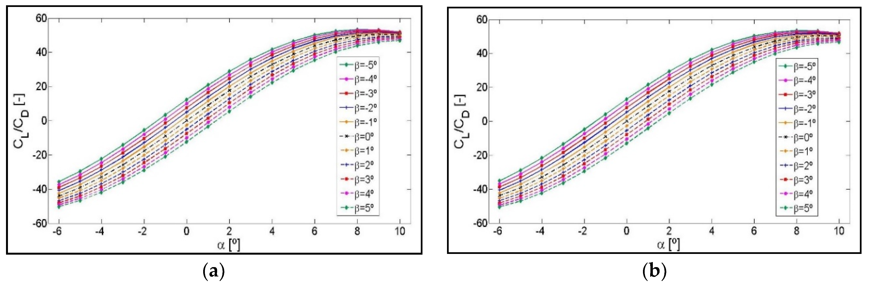
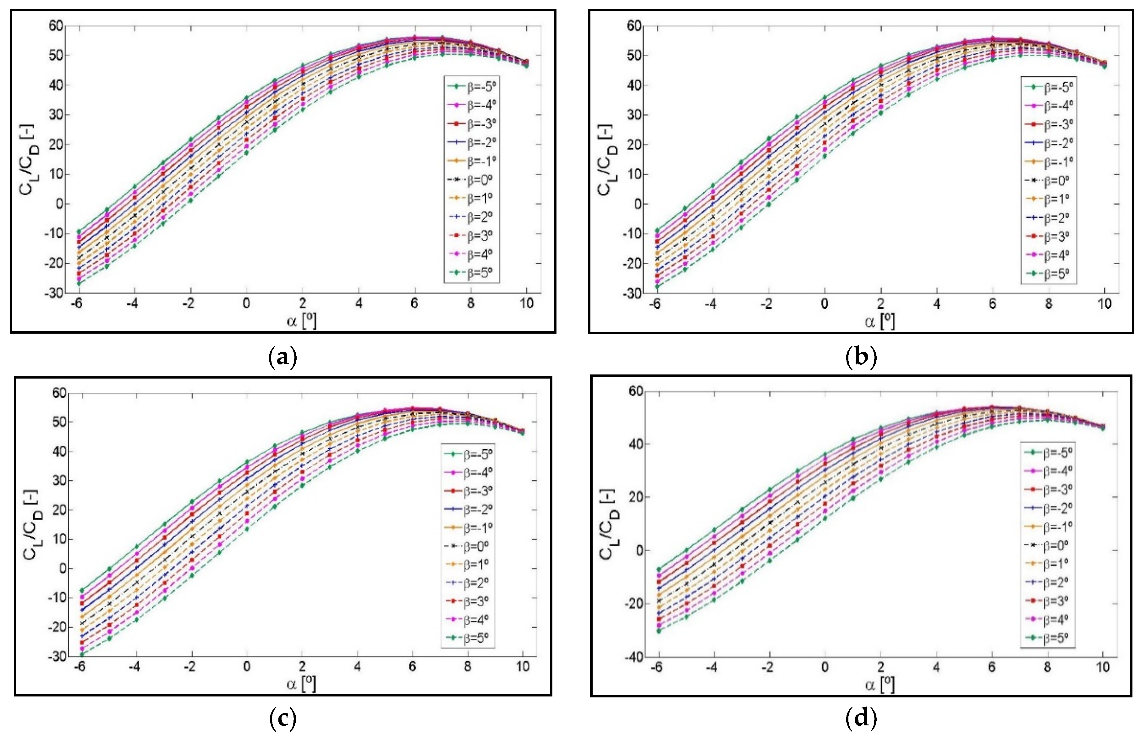
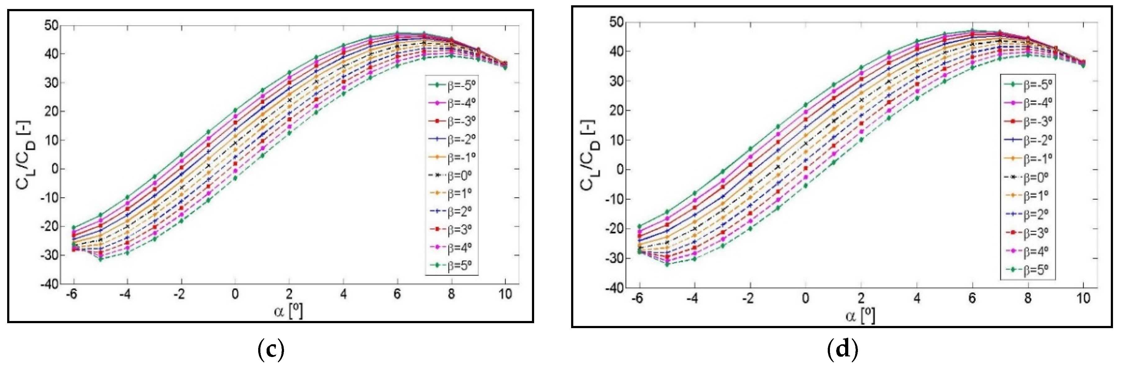
4.1. Lift-to-Drag Ratio CL/CD as a Function of the Angle of Attack, α, for Different Flap Angles β

Lift-to-drag ratio, CL/
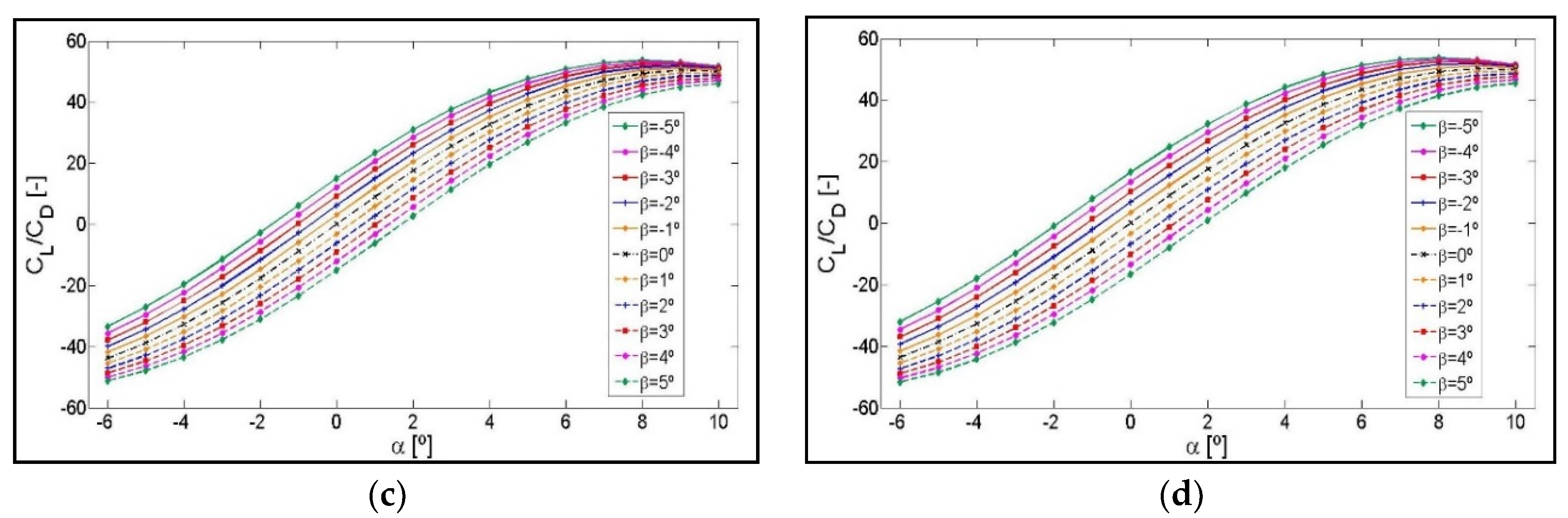
CD, as a function of the angle of attack, α, is used to show the results obtained from computational simulations. As explained in the previous section, simulations were performed for seventeen angles of attack, by combining eleven flap angles with five flaplengths. A flaplength of 8% of chord length c is chosen in this section. The curves corresponding to the rest of the flaplengths 9%, 10%, 12%, and 14% of c are included in Appendix A.
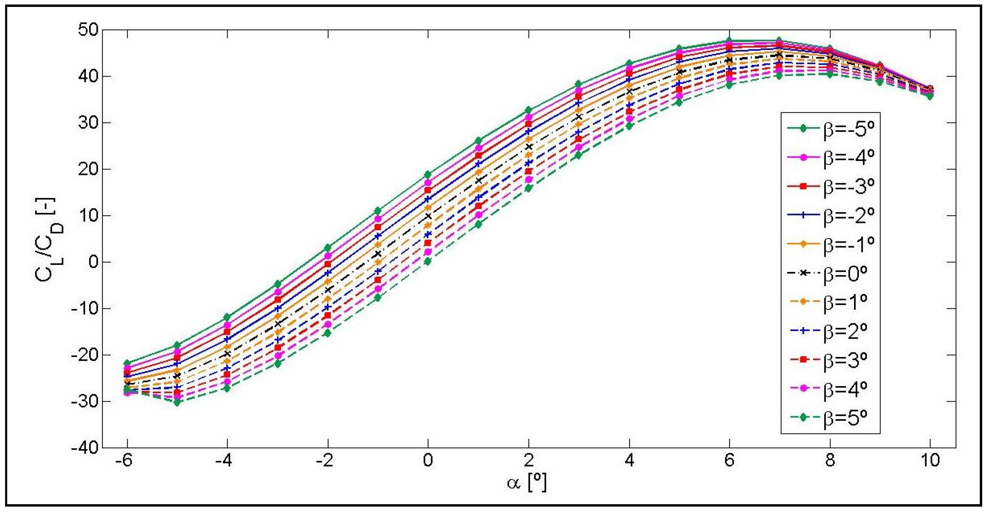
As explained in the introduction, the TEF concept is based on lift increase, when the flap is deployed on the pressure side (negative β angles), and lift decrease when the flap is deployed on the suction side (positive β angles) of the airfoil. It can therefore be deduced from the following Figure 10, Figure 11 and Figure 12, corresponding to the profiles for NACA 0012, NACA 64(3)-618, and S810, respectively, that results are in concordance with the aerodynamic results expected when studying a TEF inserted on an airfoil. As the flap is deployed towards the pressure area of the airfoil, approaching higher values of negative β angles, the lift increases. As the flap is deployed towards the suction zone of the airfoil, approaching higher values of positive β angles, the lift decreases.
As shown in the following Figure 10, Figure 11 and Figure 12 of the CL/CD curves, the CL/CD ratio of each airfoil for the same angle of attack, α, increases and it decreases as a function of the β angle in the same proportion with respect to the curve, β = 0°.
For a flap angle of β = −5°, the range of α angles of attack chosen for this study, allow obtaining a maximum lift-to-drag ratio CL/CD for the three airfoils studied. As shown in Figure 10, Figure 11 and Figure 12, depending on the flap angle, the maximum values of the CL/CD are obtained for the following intervals of the angle of attack: α = [8–10°] in the case of airfoil NACA 0012 and α = [6–8°] in the case of NACA 64(3)-618 and S810 airfoils.
As the positive and negative angle of attack, α, increases, the drag increases in a larger proportion than the lift, in such a way that when reaching the highest positive angle of attack, α = 10°, and at the highest negative angle of attack α = −6°, the CL/CD ratio values for different β angles are almost overlapping. These near overlaps are shown in Figure 10 and Figure 12, corresponding to airfoils NACA 0012 and S810, respectively, where the drag increases in the same proportion for α positive angles and for negative ones in the case of NACA 0012, and almost in the same proportion in the case of S810. However, as shown in Figure 11, drag increases substantially as the positive value of α increases for the NACA 64(3)-618 airfoil and less so when the negative value of α increases.
As shown in Figure 10, corresponding to the NACA 0012 airfoil, the CL/CD curve for the intermediate flap position β = 0° defines a symmetrically odd function as the positive and negative angle of α increases, due to the symmetry of the airfoil with respect to the horizontal Cartesian axis CL/CD = 0. However, in the case of the other two profiles, NACA 64(3)-618 and S810, there is no symmetrical evolution in the values of the curves due to the fact that they are non-symmetrical airfoils.
In addition, the CL/CD curves cross the α axis and acquire negative values at a specific value of α, in all the CL/CD curves shown in Figure 10, Figure 11 and Figure 12. A negative value of CL/CD means that the value of CL is negative. This change in the distribution of airfoil pressures happens due to a reorientation of the lift force, in such a way that as the value of the negative α angle increases, the pressure gradient in the opposite direction also increases and, consequently, the suction originates in the lower surface. The CL/CD curves acquire negative values of α ≤ 1° for the NACA 0012 airfoil, of α < −2° for the NACA 64(3)-618 airfoil, and of α ≤ 0° for the S810 airfoil. These intersection values are for a flaplength of 8% and could vary depending on the flaplength chosen for the representation of the CL/CD curves of each airfoil, as shown in Appendix A.

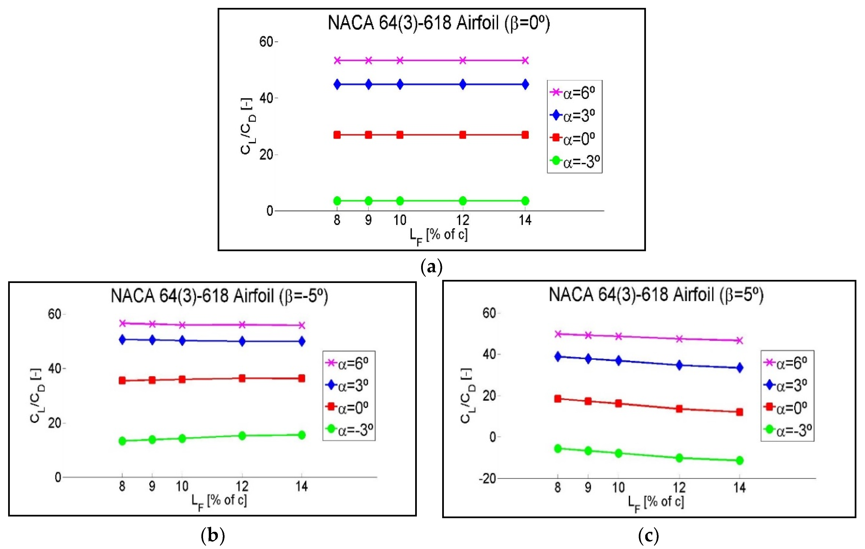
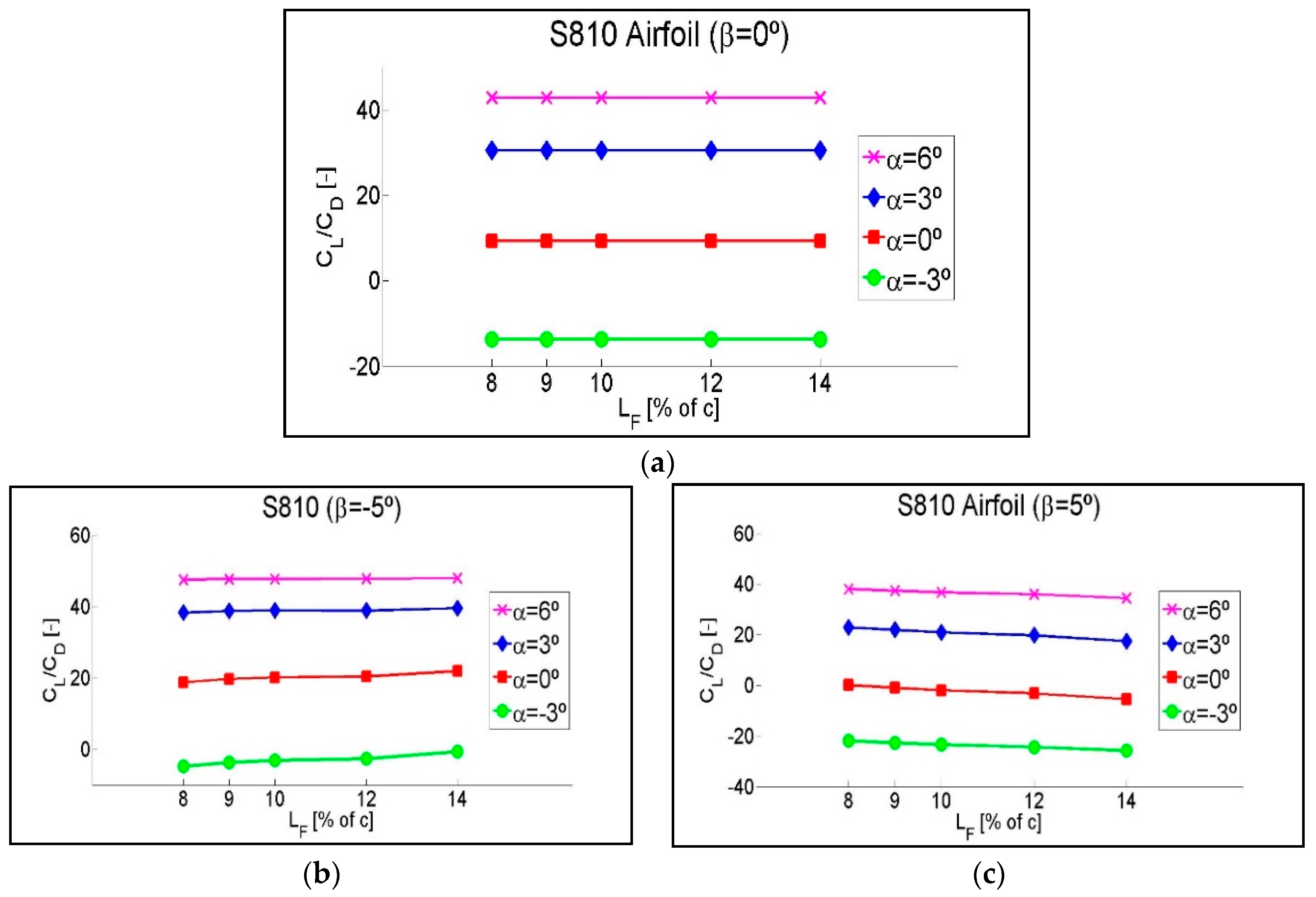
4.2. CL/CD Ratio as a Function of FlapLengths, LF, for Intermediate Angles of Attack, α

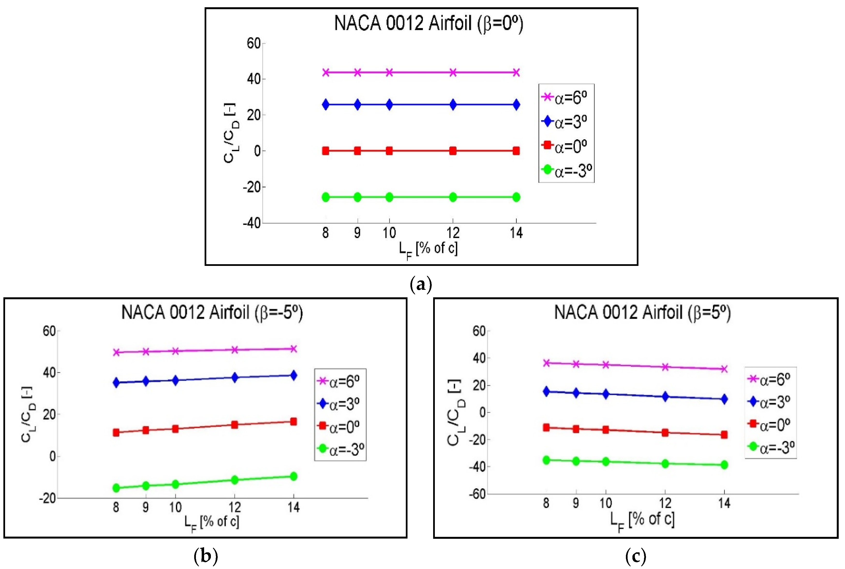
The effect of different flaplengths on the CL/CD ratio is shown in this section, with a view to defining which of them optimizes the operation of a TEF better. Three extreme flap positions were chosen for each airfoil, in order to compare the different flap lengths: flap with a position of: β = 0° (no deflection ≡ intermediate lift force); β = −5° (deflected towards the lower surface ≡ maximum lift force); and, β = 5° (deflected towards the upper surface ≡ minimum lift force).
Each plot corresponds to one of the three mentioned angles β. For each β angle, the CL/CD ratio of four intermediate angles of attack, α = −3°, α = 0°, α = 3° and α = 6°, will be compared for different flaplengths of 8%, 9%, 10%, 12%, and 14% of c.
Figure 13, corresponding to the symmetric airfoil NACA 0012, shows the variations of CL/CD of four angles of attack as a function of the different flap lengths for the angles β = 0°, β = −5°, and β = 5°, respectively.
In Figure 13a, corresponding to the flap position β = 0°, no variations of the CL/CD ratio are observed as a function of flaplength. This is because for β = 0°, the variation of flaplength does not vary the geometry of the airfoil as the flap is an integrated part of it. However, Figure 13b, corresponding to the position of flap β = −5°, clearly shows an upward trend of the CL/CD ratio for all of the four intermediate angles of attack as the flap length increases. This trend indicates that when the flap is deflected towards the lower surface in its extreme position, β = −5°, a position in which the highest lift force is obtained, the maximum CL/CD ratio is obtained with a 14% flap length. Figure 13c, corresponding to the position of flap β = 5°, shows a downward trend of the CL/CD ratio as the flap length increases. This downward trend indicates that when the flap is deflected towards the upper surface at its extreme position, β = 5°, a position in which the least lift force is obtained, the minimum CL/CD ratio is obtained with a flaplength of 14% of c. Therefore, a greater flaplength maximizes the lift in the positions in which the highest lift force is obtained, and minimizes the lift in the positions in which the lowest lift force is obtained.
The results of the NACA 64(3)-618 and the S810 airfoils, shown in Figure A4 and Figure A5 of Appendix B, are consistent with those obtained previously for the NACA 0012 airfoil, which showed the effect of different flaplengths on the aerodynamic coefficients of the airfoil. Consequently, larger flaplengths for the NACA 64(3)-618, and the S810 airfoils also maximize the CL/CD ratio in the positions in which the highest lift force is obtained and minimize it in the positions in which the lowest lift force is obtained. Moreover, as shown in plots A4 (a) and A5 (a) of Figure A4 and Figure A5, for the horizontal position of the flap, β = 0°, there is no variation of the CL/CD values as a function of flaplength either.
Figure A4b, corresponding to the NACA 64(3)-618 airfoil, with a value of α = 6°, very close to stall values, shows that when the flap is deflected towards the lower surface in its extreme position, β = −5°, as the flap length increases, the CL/CD ratio decreases slightly, instead of increasing.

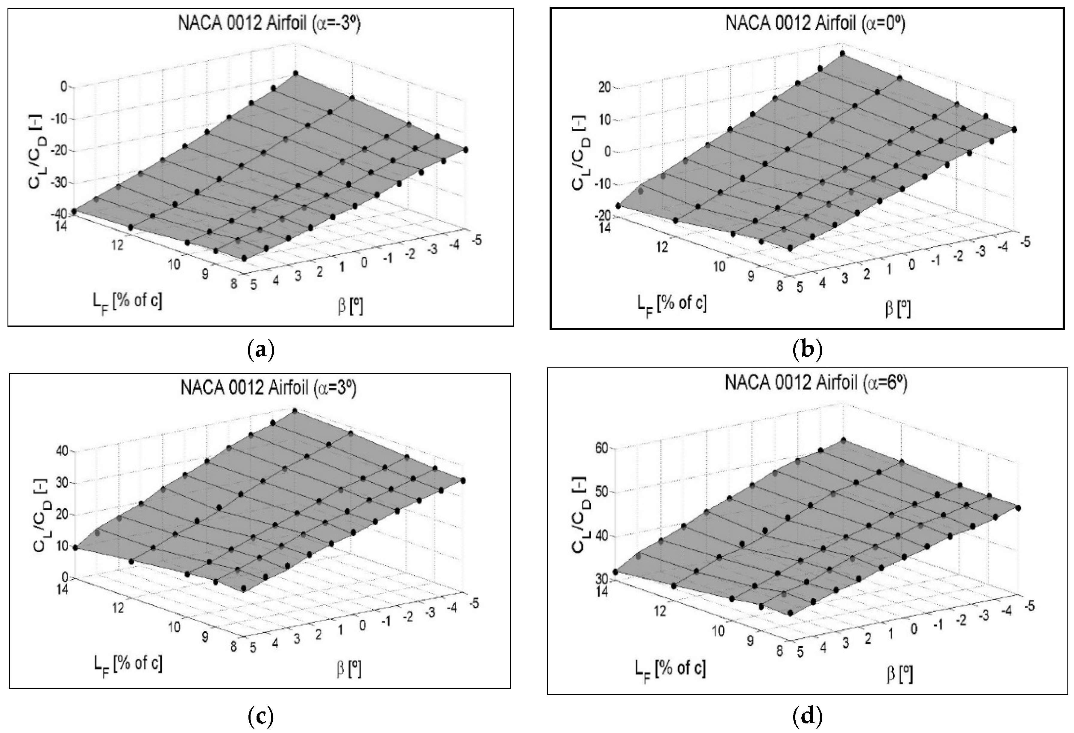
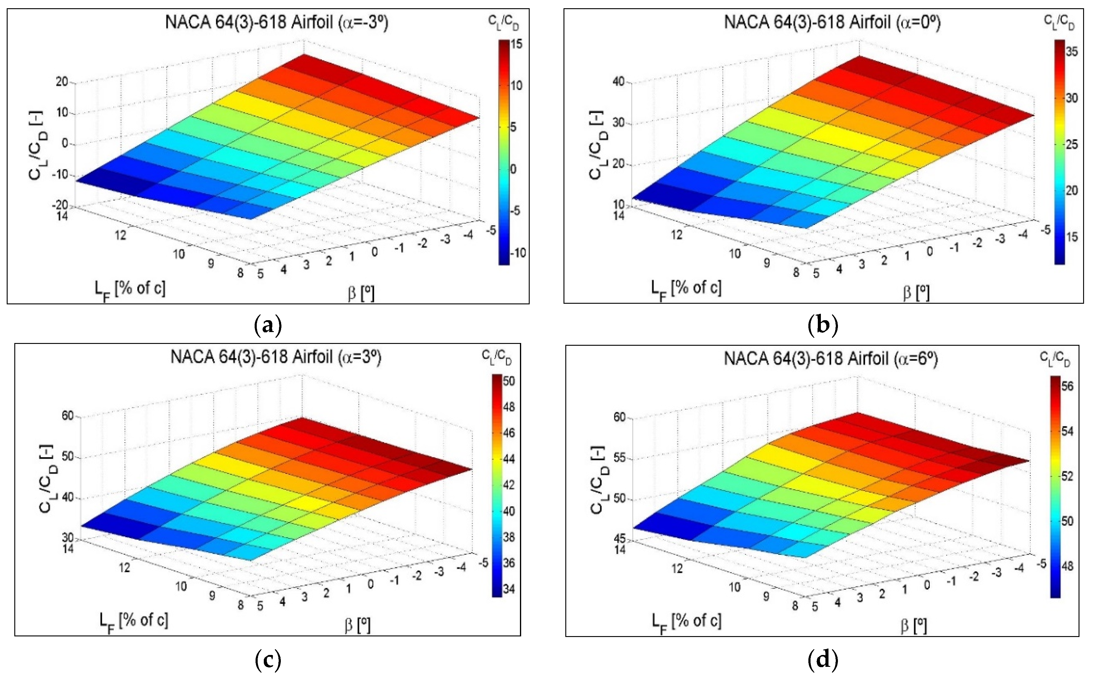
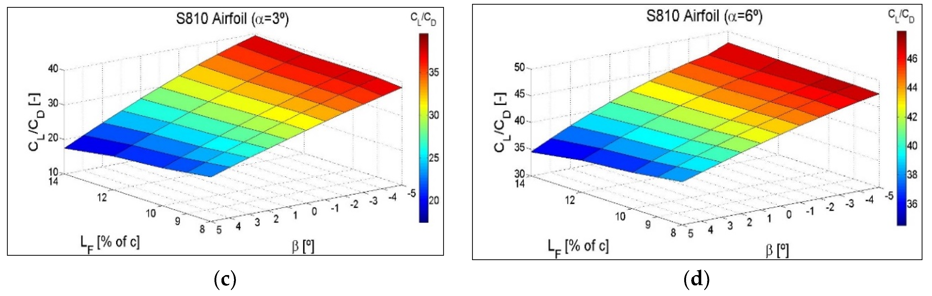
4.3. CL/CD Ratio as a Function of the Flap Angle β and the Different Flap Lengths LF

Figure 14, corresponding to the symmetric airfoil NACA 0012, at four intermediate angles of attack, α = −3°, α = 0°, α = 3° and α = 6°, shows the CL/CD ratio variation as a function of the flap angle β and the different flaplengths in the form of a three-dimensional surface. As the flap is deployed towards the pressure area of the airfoil and negative β increases, the lift increases, and the CL/CD ratio also increases. If the flap is deployed towards the suction zone and positive β increases, the lift decreases, and the CL/CD ratio also decreases. In addition, a greater flaplength maximizes the CL/CD ratio in the positions in which the highest lift force is obtained, and minimizes the CL/CD ratio in the positions in which the lowest lift force is obtained.
The same three-dimensional type of surfaces for NACA 64(3)-618 and S810 non-symmetrical airfoils are shown in Figure A6 and Figure A7 of Appendix C. The drag increases at a value of the angle of attack, α, quite close to stall values and with the flap deflected towards the pressure zone, in such a way that, as the flaplength increases at these extreme α angles, the CL/CD ratio increases less, shows no increase at all, and can even decrease.
Having studied the influence of the flap angle, β, and the flaplength, LF, on the CL/CD ratio for certain angles of attack, α, the next step will be to build a prediction model of aerodynamic forces taking into account all the parameters studied throughout this research. This model is based on an artificial neural network (ANN).

4.4. Modeling of the CFD Results with an Artificial Neural Network

Taking advantage of the results previously generated, the purpose of this section is to make a prediction model that could facilitate future computational control tools for TEFs and aerodynamic predictions tools. Bernhammer et al. [50] demonstrated the load reduction potential of smart rotors by designing an individual flap controller. In addition, the prediction model presented below could be an interesting contribution to the blade element momentum (BEM) theory. BEM theory with airfoil data is a widely used technique for prediction of wind turbine aerodynamic performance, being the reliability of the airfoil data an important factor for the prediction accuracy of aerodynamic forces and power, see Yang et al. [51].
An artificial neural network (ANN) has been designed to model the CL/CD ratio of the three different airfoils as a function of the flap angle β and the different flap lengths LF. Moreover, the ANN contains the model of the CL/CD ratio for different values of the angle of attack, α of the incoming airflow. This model was built using Matlab [52] mathematical software.
The selected topology for the ANN is the MultiLayer Perceptron with BackPropagation (MLP-BP), which is known for its good characteristics to model every surface. In the work of Aramendia et al. [53] a MLP-BP neural network is designed to model the aerodynamic behavior of a DU91W(2)250 airfoil with different length gurney flaps (GFs). A MLP-BP is presented by Saenz-Aguirre et al. [54] to store the data corresponding to the matrix Q(s,a) of a reinforcement learning algorithm for the yaw angle control of a wind turbine.
The MLP-BP designed in this paper presents one input layer with 3 neurons, corresponding to each one of the inputs (α, LF and β), one hidden layer with 25 neurons and one output layer with 1 neuron, corresponding to the output of the ANN (the CL/CD ratio). The training process of the ANN has been carried out with a data set of 220 tuples and the distribution of the data has been set to 90% for the training, 5% for the validation, and 5% for the test.
After the training, the values of the regression coefficient (R) in the test and the values for the mean squared error (MSE) have been obtained. Both are indicators of a correct training process and they are shown below in Table 4.
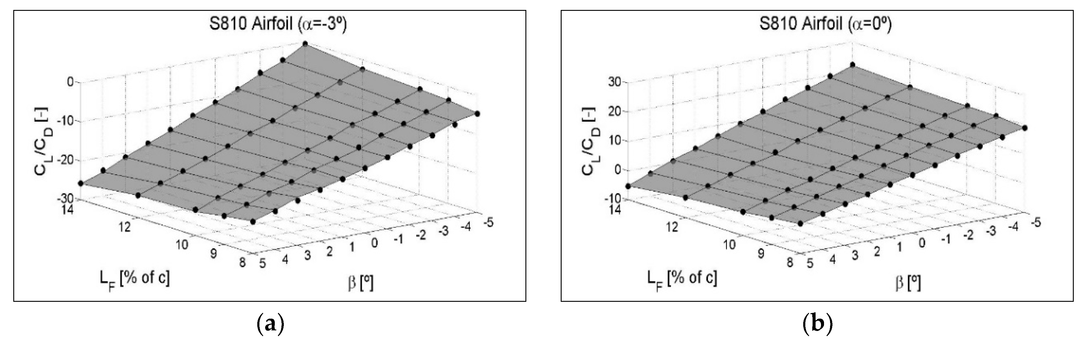
The ANN of this study and the CFD results for the airfoil NACA 0012 are shown in Figure 15. Following the procedure of a similar study carried out by Urkiola et al. [55], the model has been represented as a surface. Black dots represent the CFD results. The same comparative representations for NACA 64(3)-618 and S810 non-symmetrical airfoils are shown in Figure A8 and Figure A9 of Appendix D.
Taking into account the concurrency between CFD results and the ANN, we can confirm that the ANN model could be a good option for future computational control tools for TEFs and aerodynamic predictions tools.
Finally, with the purpose of adding more information to the results previously exposed, the results of the streamwise velocity u (ux due of α = 0°), the wake turbulence kinetic energy TKE and the pressure coefficient Cp have been studied for a select number of cases of the three airfoils NACA 0012, NACA 64(3)-618 and S810.

4.5. Streamwise Velocity

For the same angle of attack α = 0°, six different cases have been chosen for each airfoil. With the intention of covering the largest possible area of data, the minimum and maximum flaplengths of 8% of c and 14% of c with the three extreme flap positions, β = −5°, β = 0° and β = 5° have been combined.
The results corresponding to the streamwise velocity and wake turbulence kinetic energy have been checked in the following wake locations: x/c = 1.05, x/c = 1.25 and x/c = 1.5.
The data corresponding to the NACA 0012 airfoil are shown below in this results section. The data corresponding to the airfoils NACA 64(3)-618 and S810 are shown in Appendix E and Appendix F.
The results of the streamwise velocity and the wake turbulence kinetic energy, shown in Figure 16 and Figure 17 respectively, are represented in normalized form. Each figure contains three different plots. The results of the pressure coefficient are represented in a single plot of Figure 18. The normalized streamwise velocity distributed in different wake positions for three extreme flap positions and two flaplengths is shown in Figure 16a. If the curves corresponding to different wake positions are superimposed for each flaplength of 8% of c and 14% of c, enlargements of the disturbed areas are shown in Figure 16b,c, respectively.
As shown in Figure 16a, due to the reduction of the influence of the airfoil, the curves of normalized streamwise velocity furthest from the trailing edge, x/c = 1, are those that present a lesser alteration. This happens indifferently from the flaplength. The measurements of these alterations can be obtained in Figure 16b,c. The same effect for the airfoils NACA 64(3)-618 and S810 is shown in Figure A10 and Figure A12 of Appendix E.
As shown throughout the results section, also for the streamwise velocity, a greater effect is generated with a flap of 14% of c. The effect of a flaplength of 14% of c is also greater for the airfoils NACA 64(3)-618 and S810.
Because the NACA 0012 is a symmetrical airfoil, the effect generated by the two extreme flap positions of β = 5° and β = −5° is absolutely symmetric with respect to the horizontal axis. This does not happen for the NACA 64(3)-618 and S810 asymmetrical airfoils.

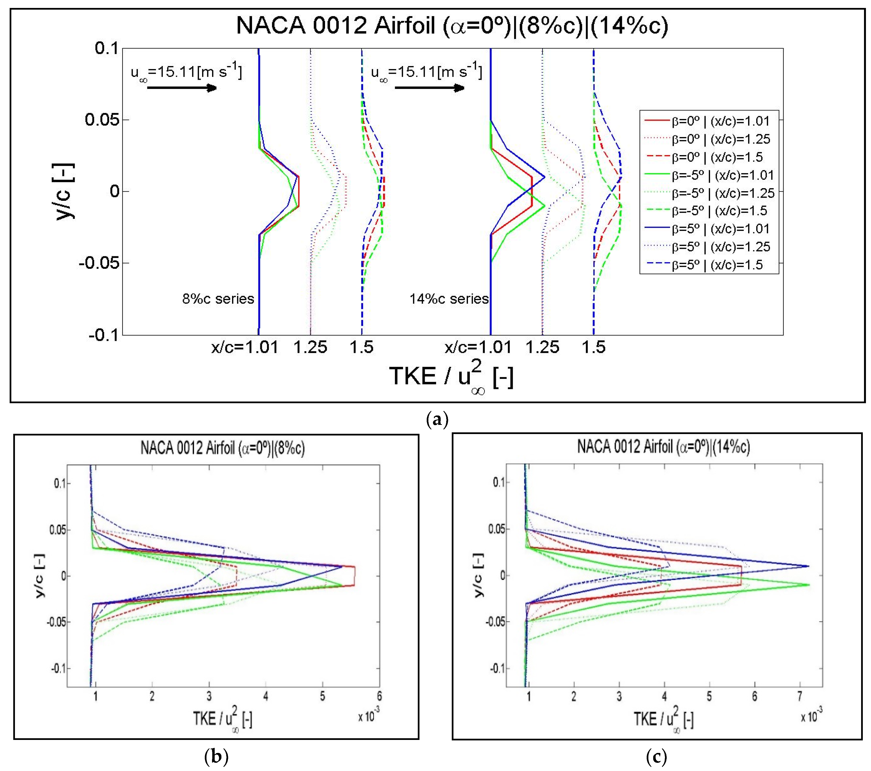
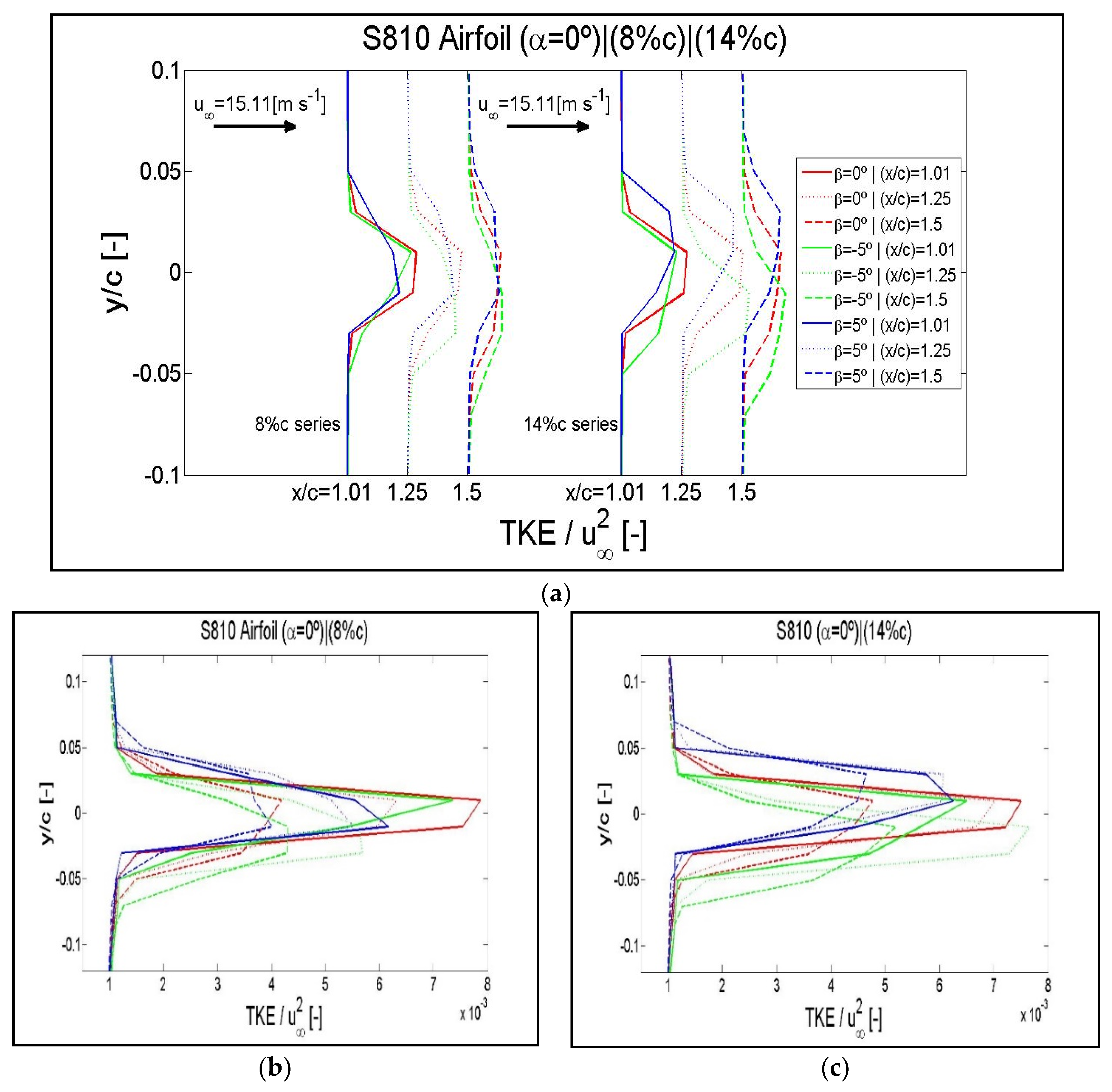
4.6. Turbulence Kinetic Energy

Then, as shown in Figure 17, the results of the normalized wake turbulence kinetic energy are displayed in the same format in which the streamwise velocity has been previously shown.
The normalized turbulence kinetic energy distributed in different wake positions for three extreme flap positions and two flaplengths is shown in Figure 17a. If the curves corresponding to different wake positions are superimposed for each flaplength of 8% of c and 14% of c, enlargements of the disturbed areas are shown in Figure 17b,c, respectively.
As for the streamwise velocity, the curves furthest from the trailing edge are those that present a lesser alteration. Also, for turbulence kinetic energy, a greater effect is generated with a flaplength of 14% of c. The effect generated by the flap positions β= 5° and β = −5° is also symmetric with respect to the horizontal axis for airfoil NACA 0012.
The results corresponding to the airfoils NACA 64(3)-618 and S810 are shown in Figure A11 and Figure A13 of Appendix E.

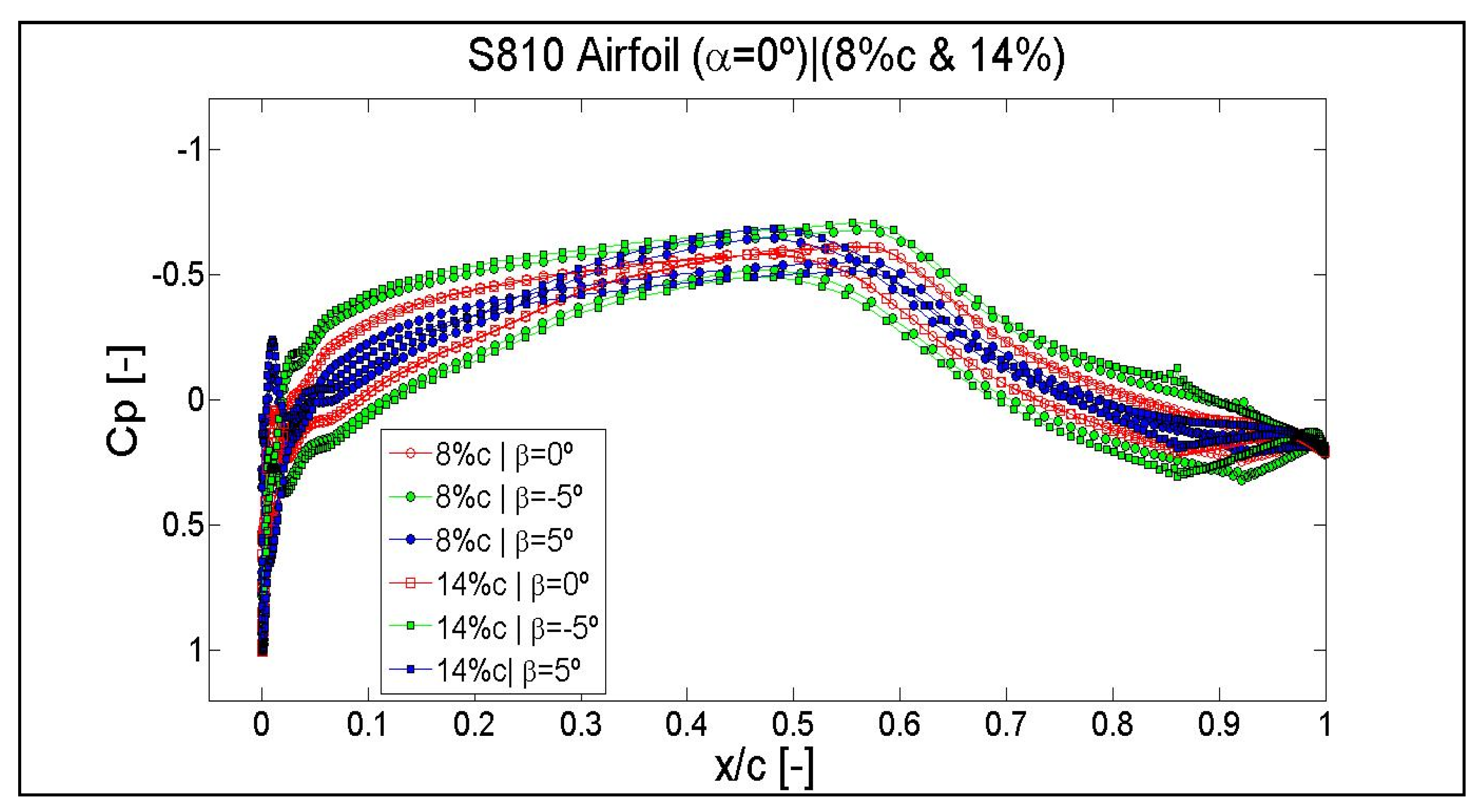
4.7. Pressure Coefficient

As shown in Figure 18, the curves of the pressure coefficient corresponding to the flap position β = 0° are coincident for the flaplengths of 8% of c and 14% of c. The curves corresponding to the flaplength of 14% of c are the ones with the greatest area of pressure.
The curves corresponding to the positions of β = 5° and β = −5° are symmetric with respect to the pressure curve β = 0°. Besides, for the same flaplength, the curves of β = 5° and β = −5° are coincident. As mentioned on previous occasions, this is a phenomenon that happens due to the symmetry of the airfoil NACA0012. As shown in Figure A14 and Figure A15 of Appendix F, this does not happen for airfoils NACA 64(3)-618 and S810.
The slight disturbance appeared between x/c = 0.25 and x/c = 0.5 reflects the laminar-turbulent transition zone.

5. Conclusions

A computational study of three airfoils, NACA 0012, NACA 64(3)-618, and S810 installed with trailing edge flaps has been performed by means of 2D computational fluid dynamic simulations at a Reynolds number of Re = 10⁶. In this work, the open source code OpenFOAM [39] was used for the simulations. The simpleFoam solver, combined with the k-ω SST turbulence model, was applied for steady-state, incompressible, and turbulent flow using RANS equations.
Having previously validated the CFD model, the procedure followed in this work has been schematically shown in Figure 3. The three different airfoils (NACA 0012, NACA 64(3)-618, and S810) have five flaplengths of 8%, 9%, 10%, 12%, and 14% of chord length c combined with eleven flap angles from β = −5° to β = 5°. The simulations have been performed for seventeen angles of attack from α = −6° to α = 10°.
The results add new knowledge about the effects of TEFs applied to three airfoil sections specifically intended for wind turbine application. This research can provide useful data for the research community in developing new blade designs and aerodynamic forces control strategies for wind turbine rotors. The obtained results are in accordance with the aerodynamic results expected when studying a TEF inserted on an airfoil.
As the flap is deployed towards the pressure area of the airfoil, reaching higher values of negative β angles, the lift increases. On the contrary, as the flap is deployed towards the suction zone of the airfoil, reaching higher values of positive β angles, the lift decreases. In addition, the results for all the three airfoils have shown that the greatest flaplength studied here maximizes the CL/CD ratio in the positions in which the highest lift force is obtained, and minimizes the CL/CD ratio in the positions in which the lowest lift force is obtained.
To show the results on which this last conclusion is based, athree-dimensional surface representing CL/CD ratio variation as a function of the flap angle β and the different flaplengths has been addressed.
The maximum values of the lift-to-drag-ratio CL/CD were obtained, with a flaplength of 14% and with a flap angle β = −5°. The maximum CL/CD ratio values are, 53.67 [-], 53.89 [-], and 46.94 [-] for the airfoils NACA 0012, NACA64(3)-618, and S810 respectively.
On the one hand, taking these results into account, aerodynamic forces reduce the blade of a wind turbine by deflection of the flap towards the suction zone, such that when positive β increases, this would be an acceptable option. On the other hand, the deflection of the flap towards the pressure zone, when positive β decreases, would be an acceptable means of increasing the output power of the turbine. The recommended flaplength in both cases would be the largest of them all, in this study 14% of c.
The prediction model built to obtain the CL/CD ratio variation of the airfoils as a function of flap angle, β, and flap length, LF, based on an ANN has been shown in Section 4.4. As the numerical and graphical results show, this approach might represent a good option to facilitate future computational automatic-control tools for TEFs installed on airfoils.
Complementary data about streamwise velocity and turbulence kinetic energy in different points of the wake region as well as pressure coefficient data added to this study can give more information and consolidate the results previously exposed.

Author Contributions

I.R.-E., I.E. and U.F.-G. prepared and ran the numerical part. I.R.-E. made the post processing and wrote the manuscript. J.M.B. and E.Z. provided constructive instructions in the process of preparing the paper. A.S.-A. wrote the ANN code used in the modeling. All authors have read and agreed to the published version of the manuscript.

Funding

The funding from the Government of the Basque Country and the University of the Basque Country UPV/EHU through the ELKARTEK kk-2016/00031 research program is gratefully acknowledged.

Conflicts of Interest

The authors declare no conflict of interest.

Nomenclature

TEFTrailing Edge Flap
DTEFDeformable Trailing Edge Flap
CFDComputational Fluid Dynamics
CLLift coefficient [-]
CDDrag coefficient [-]
αAngle of attack [deg]
βFlap angle [deg]
cAirfoil chord length [m]
LFFlaplength [% of c]
RRadius [nº of c]
UConstant velocity [m s−1]
PNo gradient pressure [N m−2]
νtTurbulent viscosity [m2 s−1]
kKinetic energy [m2 s−2]
ωDissipation rate [s−1]
ITurbulence intensity [%]
lMixing length [m]
ReReynolds number [-]
U Free stream velocity [m s−1]
ρDensity [kg m−3]
y+Dimensionless wall distance [-]
μAbsolute viscosity [kg m−1 s−1]
yFirst cell height [m]
uStreamwise velocity [m s−1]
uxx component of u [m s−1]
bSpan [m]
AArea determined by c and b [m2]
FLLift force [N]
TKETurbulence kinetic energy [m2 s−2]
CpPressure Coefficient [-]
BCBoundary Conditions
RANSReynolds Averaged Navier-Stokes
SSTShear Stress Transport
RCorrelation coefficient [-]
MSEMean Square Error [-]
ANNArtificial Neural Network
MLP-BPMulti Layer Percep.with Back Propagation
BMEBlade Element Momentum
NACANat’l Adv. Comm. of Aeronautics
NRELNat’l Renewable Energy Laboratory
HAWTHorizontal Axis Wind Turbines

Appendix A

Figure A1. Lift-to-drag ratio CL/CD curves as a function of angle of attack, α, for different angles, β. NACA 0012 airfoil with different flaplengths of: (a) 9%, (b) 10%, (c) 12% and (d) 14% of chord length c.
Symmetry 12 00828 g0a1aSymmetry 12 00828 g0a1b
Figure A2. Lift-to-drag ratio CL/CD curves as a function of angle of attack α for different angles, β. NACA 64(3)-618 Airfoil with different flaplengths of: (a) 9%, (b) 10%, (c) 12% and (d) 14% of chord length c.
Symmetry 12 00828 g0a2
Figure A3. Lift-to-drag ratio CL/CD curves as a function of angle of attack, α, for different angles, β. S810 Airfoil with different flaplengths of: (a) 9%, (b) 10%, (c) 12% and (d) 14% of chord length c.
Symmetry 12 00828 g0a3aSymmetry 12 00828 g0a3b

Appendix B

Figure A4. Variation of the CL/CD ratio as a function of different flaplengths, LF, for intermediate angles of attack, α. Rated for three different flap positions: (a) β = 0°, (b) β = −5°and (c) β = 5°. NACA 64(3)-618 Airfoil.
Symmetry 12 00828 g0a4
Figure A5. Variation of the CL/CD ratio as a function of different flaplengths LF, for intermediate angles of attack, α. Rated for three different flap positions: (a) β = 0°, (b) β = −5°and (c) β = 5°. S810 Airfoil.
Symmetry 12 00828 g0a5

Appendix C

Figure A6. CL/CD ratio variation as a function of the flap angle, β, and the different flaplengths, LF, for intermediate angles of attack: (a) α = −3°, (b) α = 0°, (c) α = 3° and (d) α = 6°. NACA 64(3)-618 Airfoil.
Symmetry 12 00828 g0a6
Figure A7. CL/CD ratio variation as a function of the flap angle, β, and the different flaplengths, LF, for intermediate angles of attack (a) α = −3°, (b) α = 0°, (c) α = 3° and (d) α = 6°. S810 Airfoil.
Symmetry 12 00828 g0a7aSymmetry 12 00828 g0a7b

Appendix D

Figure A8. The surface represents the ANN. The results of the CFD are indicated by black dots for the intermediate angles of attack (a) α = −3°, (b) α = 0°, (c) α = 3° and (d) α = 6°. NACA 64(3)-618 Airfoil.
Symmetry 12 00828 g0a8
Figure A9. The surface represents the ANN. The results of the CFD are indicated by black dots for the intermediate angles of attack (a) α = −3°, (b) α = 0°, (c) α = 3° and (d) α = 6°. S810 Airfoil.
Symmetry 12 00828 g0a9aSymmetry 12 00828 g0a9b

Appendix E

Figure A10. Results of the normalized streamwise velocity checked in the wake locations of x/c = 1.05, 1.25 and 1.5 for an angle of attack of α = 0° and flap positions of β = −5°, β = 0° and β = 5°. (a) Curves corresponding to the flaplengths of 8% of c and 14% of c distributed in the wake region. Enlargements of the disturbed areas in superimposed curves: (b) flaplength of 8% of c, (c) flaplength of 14% of c. Airfoil NACA 64(3)-618.
Symmetry 12 00828 g0a10
Figure A11. Results of the normalized wake TKE checked in the wake locations of x/c = 1.05, 1.25 and 1.5 for an angle of attack of α = 0° and flap positions of β = −5°, β = 0° and β = 5°. (a) Curves corresponding to the flaplengths of 8% of c and 14% of c distributed in the wake region. Enlargements of the disturbed areas in superimposed curves: (b) flaplength of 8% of c, (c) flaplength of 14% of c. Airfoil NACA 64(3)-618.
Symmetry 12 00828 g0a11
Figure A12. Results of the normalized streamwise velocity checked in the wake locations of x/c = 1.05, 1.25 and 1.5 for an angle of attack of α = 0° and flap positions of β = −5°, β = 0° and β = 5°. (a) Curves corresponding to the flaplengths of 8% of c and 14% of c distributed in the wake region. Enlargements of the disturbed areas in superimposed curves: (b) flaplength of 8% of c, (c) flaplength of 14% of c. Airfoil S810.
Symmetry 12 00828 g0a12
Figure A13. Results of the normalized wake TKE checked in the wake locations of x/c = 1.05, 1.25 and 1.5 for an angle of attack of α = 0° and flap positions of β = −5°, β = 0° and β = 5°. (a) Curves corresponding to the flaplengths of 8% of c and 14% of c distributed in the wake region. Enlargements of the disturbed areas in superimposed curves: (b) flaplength of 8% of c, (c) flaplength of 14% of c. Airfoil S810.
Symmetry 12 00828 g0a13

Appendix F

Figure A14. Results of the pressure coefficient Cp for an angle of attack of α = 0°, flaplengths of 8% of c and 14% of c, and flap positions of β = −5°, β = 0° and β = 5°. Airfoil NACA 64(3)-618.
Symmetry 12 00828 g0a14
Figure A15. Results of the pressure coefficient Cp for an angle of attack of α = 0°, flaplengths of 8% of c and 14% of c, and flap positions of β = −5°, β = 0° and β = 5°. Airfoil S810.
Symmetry 12 00828 g0a15

References

  1. Musial, W.; Butterfield, S.; Ram, B. Energy from Offshore Wind; Conf. Paper NREL/CP-500-39450; National Renewable Energy Lab. (NREL): Golden, CO, USA, 2006.
  2. Fichaux, N.; Beurskens, J.; Jensen, P.; Wilkes, J. Design Limits and Solutions for Very Large Wind Turbines—A 20 MW Turbine Is Feasible; Tech. Rep.: Brussels, Belgium, 2011. [Google Scholar]
  3. Barlas, T.K.; van Wingerden, W.; Hulskamp, A.W.; van Kuik, G.A.M.; Bersee, H.E.N. Smart dynamic rotor control using active flaps on a small-scale wind turbine: Aeroelastic modeling and comparison with wind tunnel measurements. Wind Energy 2013, 16, 1287–1301. [Google Scholar] [CrossRef]
  4. Veers, P.; Ashwill, T.; Sutherland, H.; Laird, D.; Lobitz, D.; Griffin, D.; Mandell, J.; Musial, W.; Jackson, K.; Zuteck, M.; et al. Trends in the design, manufacture and evaluation of wind turbine blades. Wind Energy 2003, 6, 245–259. [Google Scholar] [CrossRef]
  5. Yu, W.; Zhang, M.M.; Xu, J.Z. Effect of Smart Rotor Control Using a Deformable Trailing Edge Flap on Load Reduction under Normal and Extreme Turbulence. Energies 2012, 5, 3608–3626. [Google Scholar] [CrossRef]
  6. Barlas, T.K.; Van Kuik, G.A.M. State of the art and prospectives of smart rotor control for wind turbines. J. Phys. Conf. Ser. 2007, 75. [Google Scholar] [CrossRef]
  7. Collis, S.S.; Joslin, R.D.; Seifert, A.; Theofilis, V. Issues in active flow control: Theory, control, simulation,’ and experiment. Prog. Aerosp. Sci. 2004, 40, 237–289. [Google Scholar] [CrossRef]
  8. Fernandez-Gamiz, U.; Zulueta, E.; Boyano, A.; Ramos-Hernanz, J.A.; Manuel Lopez-Guede, J. Microtab Design and Implementation on a 5 MW Wind Turbine. Appl. Sci. 2017, 7, 536. [Google Scholar] [CrossRef]
  9. Fernandez-Gamiz, U.; Zulueta, E.; Boyano, A.; Ansoategui, I.; Uriarte, I. Five Megawatt Wind Turbine Power Output Improvements by Passive Flow Control Devices. Energies 2017, 10, 742. [Google Scholar] [CrossRef] [Green Version]
  10. Van Wingerden, J.W.; Hulskamp, A.W.; Barlas, T.; Marrant, B.; Van Kuik, G.A.M.; Molenaar, D.-P.; Verhaegen, M. On the proof of concept of a ‘smart’ wind turbine rotor blade for load alleviation. Wind Energy 2008, 11, 265–280. [Google Scholar] [CrossRef]
  11. Van Dam, C.; Berg, D.E.; Johnson, S.J. Active Load Control Techniques for Wind Turbines; Technical Report SAND2008-4809; U.S. Department of Commerce, National Technical Information Service: Springfield, VA, USA, 2008.
  12. Yagiz, B.; Kandil, O.; Pehlivanoglu, Y.V. Drag minimization using active and passive flow control techniques. Aerosp. Sci. Technol. 2012, 17, 21–31. [Google Scholar] [CrossRef]
  13. Wood, R.M. A discussion of aerodynamic control effectors (ACEs) for unmanned air vehicles (UAVs). In Proceedings of the 1st UAV Conference, Portsmouth, VA, USA, 20–23 May 2002. [Google Scholar]
  14. Aramendia-Iradi, I.; Fernandez-Gamiz, U.; Sancho-Saiz, J.; Zulueta-Guerrero, E. State of the art of active and passive flow control devices for wind turbines. DYNA 2016, 91, 512–516. [Google Scholar]
  15. Houghton, T.; Bell, K.R.W.; Doquet, M. Offshore transmission for wind: Comparing the economic benefits of different offshore network configurations. Renew. Energy 2016, 94, 268–279. [Google Scholar] [CrossRef] [Green Version]
  16. Joncas, S.; Bergsmat, O.; Beukers, A. Power regulation and optimization of offshore wind turbines through trailing edge flap control. In Proceedings of the 43rd AIAA Aerospace Sciences Meeting and Exhibit, Reno, NV, USA, 10–13 January 2005; pp. 12467–12477. [Google Scholar]
  17. Buhl, T.; Gaunaa, M.; Bak, C. Potential load reduction using airfoils with variable trailing edge geometry. J. Sol. Energy Eng. Trans. ASME 2005, 127, 503–516. [Google Scholar] [CrossRef]
  18. Barlas, T.K.; van Kuik, G.A.M. Review of state of the art in smart rotor control research for wind turbines. Prog. Aerosp. Sci. 2010, 46, 1–27. [Google Scholar] [CrossRef]
  19. Abbott, I.H.; Von Doenhoff, A.E. Theory of Wing Sections, Including a Summary of Airfoil Data; Courier Corporation: Washington, DC, USA, 1959. [Google Scholar]
  20. Abdelrahman, A.; Johnson, D.A. Development of a wind turbine test rig and rotor for trailing edge flap investigation: Static flap angles case. J. Phys. Conf. Ser. 2014, 524, 012059. [Google Scholar] [CrossRef] [Green Version]
  21. Aramendia, I.; Fernandez-Gamiz, U.; Ramos-Hernanz, J.A.; Sancho, J.; Lopez-Guede, J.M.; Zulueta, E. Flow Control Devices for Wind Turbines; Springer: Cham, Switzerland, 2017; p. 629. [Google Scholar]
  22. Johnson, S.J.; Baker, J.P.; Van Dam, C.P.; Berg, D. An overview of active load control techniques for wind turbines with an emphasis on microtabs. Wind Energy 2010, 13, 239–253. [Google Scholar] [CrossRef]
  23. Roth, D.; Enenkl, B.; Dieterich, O. Active rotor control by flaps for vibration reduction-full scale demonstrator and first flight test results. In Proceedings of the 32nd European Rotorcraft Forum, Maastricht, The Netherlands, 12–14 September 2006. [Google Scholar]
  24. Kota, S.; Hetrick, J.; Osborn, R.; Paul, D.; Pendleton, E.; Flick, P.; Tilmann, C. Design and application of compliant mechanisms for morphing aircraft structures. In Smart Structures and Materials 2003: Industrial and Commercial Applications of Smart Structures Technologies; International Society for Optics and Photonics: Washington, DC, USA, 2003; Volume 5054, pp. 24–33. [Google Scholar]
  25. Lackner, M.A.; van Kuik, G. A comparison of smart rotor control approaches using trailing edge flaps and individual pitch control. Wind Energy 2010, 13, 117–134. [Google Scholar] [CrossRef] [Green Version]
  26. Basualdo, S. Load alleviation on wind turbine blades using variable airfoil geometry. Wind Eng. 2005, 29, 169–182. [Google Scholar] [CrossRef]
  27. Andersen, P.B.; Gaunaa, M.; Bak, C.; Hansen, M.H. A Dynamic Stall Model for Airfoils with Deformable Trailing Edges. Wind Energy 2009, 12, 734–751. [Google Scholar] [CrossRef] [Green Version]
  28. Barlas, T.K.; van der Veen, G.J.; van Kuik, G.A.M. Model predictive control for wind turbines with distributed active flaps: Incorporating inflow signals and actuator constraints. Wind Energy 2012, 15, 757–771. [Google Scholar] [CrossRef]
  29. Di, G.; Wu, Z.; Huang, D. The research on active flow control method with vibration diaphragm on a NACA0012 airfoil at different stalled angles of attack. Aerosp. Sci. Technol. 2017, 69, 76–86. [Google Scholar] [CrossRef]
  30. AlMutairi, J.; Ellack, E.; AlQadi, I. Dynamics of laminar separation bubble over NACA-0012 airfoil near stall conditions. Aerosp. Sci. Technol. 2017, 68, 193–203. [Google Scholar] [CrossRef]
  31. NACA National Advisory Committee of Aeronautics. AIRFOILS|NASA. Available online: https://www.nasa.gov/image-feature/langley/100/naca-airfoils (accessed on 20 October 2018).
  32. Somers, D.M. Design and Experimental Results for the S809 Airfoil; NRELlSR-440-6918 • UC Category: 1213 • DE97000206; National Renewable Energy Lab. (NREL): Golden, CO, USA, 1997.
  33. Menon, M.; Ponta, F.; Sun, X.; Dai, Q. Aerodynamic Analysis of Flow-Control Devices for Wind Turbine Applications Based on the Trailing-Edge Slotted-Flap Concept. J. Aerosp. Eng. 2016, 29, 04016037. [Google Scholar] [CrossRef]
  34. Lutz, T.; Wolf, A. Aerodynamic and acoustic design of wind turbine airfoils with trailing-edge flap. In Proceedings of the DEWEK 2010, Bremen, Germany, 17–18 November 2010; pp. 17–18. [Google Scholar]
  35. Zhu, W.J.; Behrens, T.; Shen, W.Z.; Sorensen, J.N. Hybrid Immersed Boundary Method for Airfoils with a Trailing-Edge Flap. AIAA J. 2013, 51, 30–41. [Google Scholar] [CrossRef]
  36. Ju, Y.P.; Zhang, C.H. Multi-point robust design optimization of wind turbine airfoil under geometric uncertainty. Proc. Inst. Mech. Eng. Part A J. Power Energy 2012, 226, 245–261. [Google Scholar] [CrossRef]
  37. Douvi, E.C.; Margaris, D.P. Aerodynamic Characteristics of S809 vs. NACA 0012 Airfoil for Wind Turbine Applications. In Proceedings of the 5th International Conference from Scientific Computing to Computational Engineering, 5th IC-SCCE, Athens, Greece, 4–7 July 2012. [Google Scholar]
  38. Ramsay, R.; Hoffman, M.; Gregorek, G. Effects of Grit Roughness and Pitch Oscillations on the S810 Airfoil; NREL/TP-442-7816; National Renewable Energy Lab. (NREL): Golden, CO, USA, 1996. [CrossRef]
  39. OpenFOAM. Available online: https://openFOAM.org (accessed on 8 February 2018).
  40. Menter, F.R. Zonal Two Equation Kappa-Omega Turbulence Models for Aerodynamic Flows. In Proceedings of the NASA Technical Memorandum 103975, AIAA Fluid Dynamics Conference, Orlando, FL, USA, 6 July 1993. [Google Scholar]
  41. Kral, L. Recent experience with different turbulence models applied to the calculation of flow over aircraft components. Prog. Aerosp. Sci. 1998, 34, 481–541. [Google Scholar] [CrossRef]
  42. Gatski, T. Turbulence Modeling for Aeronautical Flows; VKI Lecture Series; von Karman Institute for Fluid Dynamics: Sint-Genesius-Rode, Belgium, 2003. [Google Scholar]
  43. UIUC Airfoil Coordinates Database. Available online: http://m-selig.ae.illinois.edu/ads/coord_database.html (accessed on 9 February 2018).
  44. Timmer, W.; Van Rooij, R. Summary of the Delft University wind turbine dedicated airfoils. Trans. Am. Soc. Mech. Eng. J. Sol. Energy Eng. 2003, 125, 488–496. [Google Scholar] [CrossRef]
  45. Sørensen, N.N.; Méndez, B.; Muñoz, A.; Sieros, G.; Jost, E.; Lutz, T.; Papadakis, G.; Voutsinas, S.; Barakos, G.N.; Colonia, S.; et al. CFD code comparison for 2D airfoil flows. J. Phys. Conf. Ser. 2016, 753, 082019. [Google Scholar] [CrossRef] [Green Version]
  46. Fincham, J.H.S.; Friswell, M.I. Aerodynamic optimisation of a camber morphing aerofoil. Aerosp. Sci. Technol. 2015, 43, 245–255. [Google Scholar] [CrossRef] [Green Version]
  47. Belamadi, R.; Djemili, A.; Ilinca, A.; Mdouki, R. Aerodynamic performance analysis of slotted airfoils for application to wind turbine blades. J. Wind Eng. Ind. Aerodyn. 2016, 151, 79–99. [Google Scholar] [CrossRef]
  48. Beans, E.; Jakubowski, G. Method for Estimating the Aerodynamic Coefficients of Wind Turbine-Blades at High Angles of Attack. J. Energy 1983, 7, 747–749. [Google Scholar] [CrossRef]
  49. Young, A.D. The Calculation of Total and Skin Friction Drags of Bodies of Revolution at Zero Incidence; ARC R & M.; No. 1874: London, UK, 1939. [Google Scholar]
  50. Bernhammer, L.O.; van Kuik, G.A.M.; De Breuker, R. Fatigue and extreme load reduction of wind turbine components using smart rotors. J. Wind Eng. Ind. Aerodyn. 2016, 154, 84–95. [Google Scholar] [CrossRef]
  51. Yang, H.; Shen, W.; Xu, H.; Hong, Z.; Liu, C. Prediction of the wind turbine performance by using BEM with airfoil data extracted from CFD. Renew. Energy 2014, 70, 107–115. [Google Scholar] [CrossRef]
  52. Moler, C. MATLAB and Statistics Toolbox; The MathWorks, Inc.: Natick, MA, USA, 2013; Available online: https://es.mathworks.com/products/matlab.html (accessed on 20 October 2018).
  53. Aramendia, I.; Fernandez-Gamiz, U.; Zulueta, E.; Saenz-Aguirre, A.; Teso-Fz-Betono, D. Parametric Study of a Gurney Flap Implementation in a DU91W(2)250 Airfoil. Energies 2019, 12, 294. [Google Scholar] [CrossRef] [Green Version]
  54. Saenz-Aguirre, A.; Zulueta, E.; Fernandez-Gamiz, U.; Lozano, J.; Manuel Lopez-Guede, J. Artificial Neural Network Based Reinforcement Learning for Wind Turbine Yaw Control. Energies 2019, 12, 436. [Google Scholar] [CrossRef] [Green Version]
  55. Urkiola, A.; Fernandez-Gamiz, U.; Errasti, I.; Zulueta, E. Computational characterization of the vortex generated by a Vortex Generator on a flat plate for different vane angles. Aerosp. Sci. Technol. 2017, 65, 18–25. [Google Scholar] [CrossRef]
Figure 1. Detailed sketch of the airfoils with TEF installed and analyzed in this study where c, β, α, and LF are the airfoil chord length, the flap angle, the angle of attack, and the flaplength, respectively.
Symmetry 12 00828 g001
Figure 2. Outline of the three aerodynamic profiles used in the current work.
Symmetry 12 00828 g002
Figure 3. Procedure sketch showing the different combinations between flaplength, flap angle, and angle of attack for the airfoil NACA 0012.
Symmetry 12 00828 g003
Figure 4. Domain used for the numerical simulations in this study with an enlargement view of the airfoil in the center of the domain.
Symmetry 12 00828 g004
Figure 5. Mesh snapshots around the trailing edge flap for two different flap positions: (a) β = 5°and (b) β = −5°. Mean camber line has been added in dashed lines. Airfoil NACA 0012.
Symmetry 12 00828 g005
Figure 6. Wall y+ distribution over the airfoil for an angle of attack of α = 0°, flaplength of 8% of chord length c and two different flap positions: (a) β = 5°and (b) β = −5°. Airfoil NACA 0012.
Symmetry 12 00828 g006
Figure 7. Comparison between experimental data and CFD data for NACA 0012: (a) lift coefficient CL against angle of attack α; (b) drag coefficient CD against lift coefficient CL.
Symmetry 12 00828 g007
Figure 8. Comparison between experimental data and CFD data for NACA 64(3)-618: (a) lift coefficient CL against angle of attack α; (b) drag coefficient CD against lift coefficient CL.
Symmetry 12 00828 g008
Figure 9. Comparison between experimental data and CFD data for S810: (a) lift coefficient CL against angle of attack α; (b) drag coefficient CD against lift coefficient CL.
Symmetry 12 00828 g009
Figure 10. Lift-to-drag ratio CL/CD curves as a function of the angle of attack, α, for different angles β. The NACA 0012 airfoil with a flap length of 8% of chord length c.
Symmetry 12 00828 g010
Figure 11. Lift-to-drag ratio CL/CD curves as a function of the angle of attack, α, for different angles β. The NACA 64(3)-618 airfoil with a flap length of 8% of chord length c.
Symmetry 12 00828 g011
Figure 12. Lift-to-drag ratio CL/CD curves as a function of the angle of attack, α, for different angles β. The S810 airfoil with a flap length of 8% of chord length c.
Symmetry 12 00828 g012
Figure 13. Variation of the CL/CD ratio as a function of different flaplengths, LF, for intermediate angles of attack, α. Rated for three different flap positions: (a) β = 0°, (b) β = −5°, and (c) β = 5°. NACA 0012 Airfoil.
Symmetry 12 00828 g013
Figure 14. CL/CD ratio variation as a function of the flap angle β and the different flaplengths LF for intermediate angles of attack (a) α = −3°, (b) α = 0°, (c) α = 3° and (d) α = 6°. NACA 0012 Airfoil.
Symmetry 12 00828 g014
Figure 15. The surface represents the ANN. The results of the CFD are indicated by black dots for the intermediate angles of attack (a) α = −3°, (b) α = 0°, (c) α = 3° and (d) α = 6°. NACA 0012 Airfoil.
Symmetry 12 00828 g015
Figure 16. Results of the normalized streamwise velocity checked in the wake locations of x/c = 1.05, 1.25 and 1.5 for an angle of attack of α = 0° and flap positions of β = −5°, β = 0° and β = 5°. (a) Curves corresponding to the flaplengths of 8% of c and 14% of c distributed in the wake region. Enlargements of the disturbed areas in superimposed curves: (b) flaplength of 8% of c, (c) flaplength of 14% of c. Airfoil NACA 0012.
Symmetry 12 00828 g016
Figure 17. Results of the normalized wake TKE checked in the wake locations of x/c = 1.05, 1.25 and 1.5 for an angle of attack of α = 0° and flap positions of β = −5°, β = 0° and β = 5°. (a) Curves corresponding to the flaplengths of 8% of c and 14% of c distributed in the wake region. Enlargements of the disturbed areas in superimposed curves: (b) flaplength of 8% of c, (c) flaplength of 14% of c. Airfoil NACA 0012.
Symmetry 12 00828 g017
Figure 18. Results of the pressure coefficient Cp for an angle of attack of α = 0°, flaplengths of 8% of c and 14% of c, and flap positions of β = −5°, β = 0° and β = 5°. Airfoil NACA 0012.
Symmetry 12 00828 g018
Table 1. Summary of the results of orthogonality and skewness mesh quality parameters.
β [°]Non-Orthogonality (Average)Maximum Skewness
NACA 0012−527.700.54
027.680.49
+527.700.54
NACA 64(3)-618−522.280.87
022.160.79
+522.110.85
S810−526.390.67
026.330.61
+526.320.67
Table 2. Value of the different variables that are part of the calculation of the Reynolds number.
Reynolds Number [-]ρ [kg m−3]μ [kg m−1 s−1]c [m] U [m s−1]
1061.2251.8375 × 10−5115.11
Table 3. Summary of the non-dimensional wall y+ parameters results.
β [°]Wall y+ [-]
MinAverageMax
NACA 0012−50.020.551.29
00.020.551.18
50.020.551.09
NACA 64(3)-618−50.010.560.95
00.010.571.02
50.020.591.09
S810−50.020.681.15
00.020.671.11
50.020.681.06
Table 4. Regression coefficient (R) and Root Mean Square Error (RMSE).
AirfoilR [-]MSE [-]
NACA00120.99950.0248
NACA 64(3)-6180.99980.0173
S8100.999860.0165

