Optimal Investment, Consumption and Leisure with an Option to File for Bankruptcy

Abstract

This paper investigates the optimal personal bankruptcy decision of a debtor who participates in the labor market. This paper is based on a mathematical finance model that assumes a Black-Scholes financial market and describes a decision problem as an expected discounted utility maximization problem. Our optimization problem can be cast into a mixed optimal stopping and control problem, and has a symmetry feature with a voluntary retirement decision problem in characterizing the stopping times. To obtain value function and optimal strategies, we use dynamic programming method and transform the relevant nonlinear Bellman equation into a linear equation. Numerical illustrations from our explicit expressions for the optimal strategies reveal how an opportunity to file for bankruptcy affects debtor’s consumption, leisure, and portfolio decisions.

1. Introduction

Bankruptcy laws in the United States allow overburdened debtors to file for bankruptcy and to get a fresh financial start (Chapter 7) or reorganize debts (Chapter 13). If a debtor files for bankruptcy under Chapter 7, unsecured debts are wiped out in exchange for nonexempt assets and the debtor is allowed to keep future incomes. Chapter 13 petitioners retain all of the assets and should repay their debts over a 3–5 year period.

There is a plenty of economic literature on personal bankruptcy. Reference [1] argued that the dramatic rise of personal bankruptcy in the U.S. was due to the changes in social norms, and [2] attributed it to the expansion of credit card borrowing. How the bankruptcy protection affects on consumers was investigated by [3] (bankruptcy protection increase earnings and employment) and [4] (role of bankruptcy protection as implicit health insurance). Empirical studies [5,6,7] revealed that filers have restrictions on access to credit markets.

On the other hand, personal bankruptcy decision problem, unlike retirement decision problem, receives little attention in mathematical finance literature. Optimal retirement problem attracts enormous interests in mathematical finance literature as well as in economics literature, for examples [8,9,10,11,12,13,14] and others. Our personal bankruptcy decision problem, however, can also be cast into optimal stopping problems, which is the same as an agent’s voluntary retirement problem. The symmetry feature between personal bankruptcy and voluntary retirement can be found in manners that characterize the stopping times. The former characterizes it as the first hitting time the wealth level reaches a certain wealth threshold from above, the latter does it from below.

The first mathematical treatment of personal bankruptcy decision problem is provided in [15], which uses dynamic programming method to solve the optimization problem of a debtor who is not a wage earner. Recently, [16] considers the case where a Chapter 7 filer faces borrowing constraints against future labor income and solves utility maximization problem using martingale and duality method. In [16], the debtor is a wage earner with a fixed labor income stream, i.e., the debtor’s labor supply (or leisure rate) is not a control variable.

This paper investigates the optimal consumption, leisure, portfolio, and bankruptcy, assuming that the debtor is eligible for Chapter 7 bankruptcy. Numerous empirical studies have investigated the personal bankruptcy and labor supply (see [3,17,18,19]). All of them discuss how the debt relief have impacts on the post-bankruptcy consumer’s labor supply. However, to the best of our knowledge, there are little empirical studies for the effects of personal bankruptcy option on pre-bankruptcy debtor’s consumption, portfolio, and labor supply. An intuition is that with an option to file for bankruptcy the debtor tends supply less labor than he/she does without such an option. The aim and contribution of this paper is to justify this intuition based on a quantitative method. Our numerical illustrations based on the explicit solution we derived reveal that a debtor with an option to file for bankruptcy tends to enjoy more consumption, supply less labor and reduce savings comparing to a debtor without such an option. Moreover, with an option to file for bankruptcy the debtor tends to invest more in the risky asset than he/she does without the option. Although we have little empirical results available for our analysis, we believe this study contributes to providing an implication for policy making.

The utility is derived from consumption and leisure and has a form of Cobb-Douglas function. The Cobb-Douglas function is well suited for considering utility from consumption/leisure and is popularly accepted by many researchers in this field (for example see [11,12]). In addition, the Cobb-Douglas utility function capture consumption jump at the optimal stopping times, such as retirement time or bankruptcy time. A dynamic programming method is applied to obtain value functions and explicit forms of the optimal strategies. Numerical illustrations with our solution show the effects of an option to file for bankruptcy on debtor’s consumption, portfolio, and leisure: with an option to file for bankruptcy, he/she enjoys more consumption, leisure and invests more in the risky asset than he/she does without such an option.

The paper proceeds as follows. Section 2 introduces our markets and utility function. Section 3 defines maximization problems and solves them. Section 4 exhibits numerical results from our explicit solutions and derives the effects of an option to file for bankrputcy, and Section 5 concludes.

2. The Model

2.1. The Markets

We consider an infinitely lived debtor who participates in the financial market and the labor market. We assume a Black-Scholes financial market with constrant coefficients. The financial market consists of a money market account (riskless asset) and a risky asset. The price of money market account $\mathbf{M}:={\left(M_t\right)}_{\{t\ge 0\}}$ follows

$$d{M}_t/M_t=rdt,$$

where $r>0$ is a constant risk-free interest rate. The risky asset price $\mathbf{S}:={\left(S_t\right)}_{\{t\ge 0\}}$ evolves according to the following equation

$$\frac{d{S}_t}{S_t}=\mu dt+\sigma d{B}_t,$$

where ${\left(B_t\right)}_{t\ge 0}$ is a standard Brownian on a probability space $(\Omega ,\mathcal{F},\mathbb{P}).$ Denote by ${\left({\mathcal{F}}_t\right)}_{t\ge 0}$ the $\mathbb{P}$-augmentation of the natural filtration generated by ${\left(B_t\right)}_{t\ge 0}$. The drift $\mu (>r)$ and the volatility $\sigma$ of the risky assets are constants. Let $\mathbf{\pi }:={\left({\pi }_t\right)}_{\{t\ge 0\}}$ (call portfolio process) be the amount of money invested in the risky asset, and $\mathbf{c}:={\left(c_t\right)}_{\{t\ge 0\}}$ (call consumption process) be the nonnegative rate of consumption. The debtor’s participation in the labor market is characterized in terms of her choice of leisure. If the sum of labor rate and leisure rate is a constant $\overline{L}$, the income rate is given by $w(\overline{L}-l_t)$, where $\mathbf{l}:={\left(l_t\right)}_{\{t\ge 0\}}$ (call leisure process) is the leisure rate, and w is the wage rate. The debtor supplies a minimum level of labor rate $w(\overline{L}-L),\overline{L}>L>0,$ and thereby we will have $0\le l_t\le L.$ We assume that $\mathbf{\pi },\mathbf{c},$ and $\mathbf{l}$ are ${\mathcal{F}}_t$-progressively measurable and

$${\int }_0^t{\pi }_s^{2}ds<\infty \mathrm{for}\mathrm{all}t\ge 0a.s.,{\int }_0^t{c}_{s}ds<\infty ,\mathrm{for}\mathrm{all}t\ge 0a.s.,{\int }_0^t{l}_{s}ds<\infty \mathrm{for}\mathrm{all}t\ge 0a.s.$$

(1)

2.2. Utility Function

We employ a Cobb-Douglas utility function as the debtor’s utility function of consumption and leisure as follows

$$u(c,l)=\frac{1}{\alpha }·\frac{{\left(c^{\alpha }{l}^{1-\alpha }\right)}^{1-{\gamma }^{\ast }}}{1-{\gamma }^{\ast }},0<\alpha <1,{\gamma }^{\ast }>0({\gamma }^{\ast }\ne 1),$$

(2)

where ${\gamma }^{\ast }$ is the coefficient of relative risk aversion for consumption and leisure. $\alpha$ measures the contribution of consumption to the debtor’s utility. If we define define $\gamma :=1-\alpha (1-{\gamma }^{\ast })$, the utility function in Equation (2) can be rewritten as

$$u(c,l)=\frac{c^{1-\gamma }{l}^{\gamma -{\gamma }^{\ast }}}{1-\gamma }.$$

3. The Optimization Problems and Solution

Under Chapter 7, unsecured debts are discharged but nonexempt assets should be relinquished to the bankruptcy trustee who will liquidate them to repay creditors. To reconcile this Chapter 7 bankruptcy rule with our model, we postulate that if the debtor files for bankruptcy, the debtor (hence becomes a filer) retains some proportion $ϵ$ of wealth less a fixed cost $\nu$. Let $\mathbf{X}:={\left(X_t\right)}_{\{t\ge 0\}}$ be the wealth level and $\tau$ be the time of filing for Chapter 7 bankruptcy. Then we have

$$X_{{\tau }_{+}}=ϵ(X_{\tau }-\nu ),0\le ϵ\le 1,\nu >0.$$

After filing for Chapter 7 bankruptcy, the debtor is allowed to keep future incomes. We assume that the debtor and the filer have the same labor market parameters. Before filing for bankruptcy, the debtor repays a debt at a constant rate p. Therefore, the wealth level process satisfies the following equation

$$\begin{array}{c}\hfill d{X}_t=\left\{\begin{array}{cc}\left[r{X}_t+{\pi }_t(\mu -r)-c_t+w(\overline{L}-l_t)-p\right]dt+\sigma {\pi }_{t}d{B}_t,& t\le \tau ,\\ \left[r{X}_t+{\pi }_t(\mu -r)-c_t+w(\overline{L}-l_t)\right]dt+\sigma {\pi }_{t}d{B}_t.& t>\tau .\end{array}\right.\end{array}$$

Remark 1.

We define $\theta :=(\mu -r)/\sigma$ and consider two roots $m_{+}>0$ and $m_{-}<-1$ of the equation

$$\frac{1}{2}{\theta }^2{m}^2+\left(\beta -r+\frac{1}{2}{\theta }^2\right)m-r=0,$$

for solutions to the optimization problems.

Assumption 1.

$$K^{\ast }:=r+\frac{\beta -r}{{\gamma }^{\ast }}+\frac{{\gamma }^{\ast }-1}{2{\left({\gamma }^{\ast }\right)}^2}{\theta }^2>0,K:=r+\frac{\beta -r}{\gamma }+\frac{\gamma -1}{2{\gamma }^2}{\theta }^2>0.$$

3.1. Filer’s Optimization Problem

Firstly, we will derive the filer’s value function $V_F$ and optimal strategies. The filer’s wealth level process evolves according to the following equation

$$d{X}_t=\left[r{X}_t+{\pi }_t(\mu -r)-c_t+w(\overline{L}-l_t)\right]dt+\sigma {\pi }_{t}d{B}_t,t\ge 0,X_0=x.$$

Definition 1.

We call $(\mathbf{c},\mathbf{\pi },\mathbf{l})$ an admissible policy for a filer at x if

(a) 

c, $\mathbf{\pi }$, and $\mathbf{l}$ satisfy Equation (1),

(b) 

${\displaystyle X_t\ge -\frac{w}{r}\overline{L},t\ge 0,}$

(c) 

${\displaystyle \mathbb{E}{\int }_0^{\infty }{e}^{-\beta t}\left|u(c_t,l_t)\right|dt<\infty .}$

Let ${\mathcal{A}}_F\left(x\right)$ be the set of all admissible policies for a filer at x. Then the value function $V_F$ is defined as follows

$$V_F\left(x\right)=\underset{(\mathbf{c},\mathbf{\pi },\mathbf{l})\in {\mathcal{A}}_F\left(x\right)}{max}\mathbb{E}\left[{\int }_0^{\infty }{e}^{-\beta t}u(c_t,l_t)dt\right]=\underset{(\mathbf{c},\mathbf{\pi },\mathbf{l})\in {\mathcal{A}}_F\left(x\right)}{max}\mathbb{E}\left[{\int }_0^{\infty }{e}^{-\beta t}\frac{c_t^{1-\gamma }{l}_t^{\gamma -{\gamma }^{\ast }}}{1-\gamma }dt\right].$$

Before we state the filer’s value function and optimal strategies, we define the following constants and functions

$$\begin{array}{cc}\hfill \tilde{c}& :=\left(\frac{w\alpha }{1-\alpha }\right)L,\hfill \\ \hfill A& :=\frac{{\tilde{c}}^{{\gamma }^{\ast }{m}_{-}}}{{\gamma }^{\ast }\gamma (m_{+}-m_{-})}\left\{(1+\gamma m_{+})\frac{{\gamma }^{\ast }}{K}\tilde{c}-(1+{\gamma }^{\ast }{m}_{+})\frac{\gamma }{\alpha K^{\ast }}\tilde{c}+\frac{wL}{r}{\gamma }^{\ast }\gamma m_{+}\right\},\hfill \\ \hfill B& :=\frac{{\tilde{c}}^{\gamma m_{+}}}{{\gamma }^{\ast }\gamma (m_{+}-m_{-})}\left\{(1+\gamma m_{-})\frac{{\gamma }^{\ast }}{K}\tilde{c}-(1+{\gamma }^{\ast }{m}_{-})\frac{\gamma }{\alpha K^{\ast }}\tilde{c}+\frac{wL}{r}{\gamma }^{\ast }\gamma m_{-}\right\},\hfill \\ \hfill X_F^l\left(c\right)& :=A{c}^{-{\gamma }^{\ast }{m}_{-}}+\frac{1}{\alpha K^{\ast }}c-\frac{w\overline{L}}{r},\hfill \\ \hfill X_F^L\left(c\right)& :=B{c}^{-\gamma m_{+}}+\frac{1}{K}c-\frac{w(\overline{L}-L)}{r},\hfill \\ \hfill {\Phi }_l\left(c\right)& {\displaystyle :={\left(\frac{w\alpha }{1-\alpha }\right)}^{{\gamma }^{\ast }-\gamma }\left[\frac{r-\frac{1}{2}{\theta }^2{m}_{-}}{\beta }A{c}^{-{\gamma }^{\ast }(m_{-}+1)}+\frac{1}{K^{\ast }(1-\gamma )}{c}^{1-{\gamma }^{\ast }}\right],}\hfill \\ \hfill {\Phi }_L\left(c\right)& {\displaystyle :=L^{-({\gamma }^{\ast }-\gamma )}\left[\frac{r-\frac{1}{2}{\theta }^2{m}_{+}}{\beta }B{z}^{-\gamma (m_{+}+1)}+\frac{1}{K(1-\gamma )}{z}^{1-\gamma }\right].}\hfill \end{array}$$

Theorem 1.

The filer’s value function $V_F$ is given by

$$\begin{array}{c}\hfill V_F\left(x\right)=\left\{\begin{array}{c}{\displaystyle {\Phi }_l\left(C_F^l\left(x\right)\right)for-\frac{w\overline{L}}{r}\le x<\tilde{x},}\hfill \\ {\Phi }_L\left(C_F^L\left(x\right)\right)forx\ge \tilde{x},\hfill \end{array}\right.\end{array}$$

where $C_F^l(·)$ and $C_F^L(·)$ are the inverse functions of $X_F^l(·)$ and $X_F^L(·)$, respectively, and $\tilde{x}$ is given by

$$\tilde{x}=X_F^l\left(\tilde{c}\right).$$

Moreover, the filer’s optimal strategies $({\mathbf{c}}^{\ast },{\mathbf{\pi }}^{\ast },{\mathbf{l}}^{\ast })$ are given as follows

$$\begin{array}{c}\hfill \left\{\begin{array}{cc}{c}_t^{\ast }=C_F^l\left(X_t\right),\hfill & {\displaystyle -\frac{w\overline{L}}{r}\le X_t<\tilde{x},}\hfill \\ {\displaystyle {\pi }_t^{\ast }=\frac{\theta }{{\gamma }^{\ast }\sigma }\left\{-{\gamma }^{\ast }{m}_{-}A{C}_F^l{\left(X_t\right)}^{-{\gamma }^{\ast }{m}_{-}}+\frac{1}{\alpha K^{\ast }}{C}_F^l\left(X_t\right)\right\},}\hfill & {\displaystyle -\frac{w\overline{L}}{r}\le X_t<\tilde{x},}\hfill \\ {\displaystyle l_t^{\ast }={\left(\frac{w\alpha }{1-\alpha }\right)}^{-1}{C}_F^l\left(X_t\right),}\hfill & {\displaystyle -\frac{w\overline{L}}{r}\le X_t<\tilde{x},}\hfill \end{array}\right.\end{array}$$

$$\begin{array}{c}\hfill \left\{\begin{array}{cc}{c}_t^{\ast }=C_F^L\left(X_t\right),\hfill & {\displaystyle X_t\ge \tilde{x},}\hfill \\ {\displaystyle {\pi }_t^{\ast }=\frac{\theta }{\gamma \sigma }\left\{-\gamma m_{+}B{C}_F^L{\left(X_t\right)}^{-\gamma m_{+}}+\frac{1}{K}{C}_F^L\left(X_t\right)\right\},}\hfill & {\displaystyle X_t\ge \tilde{x},}\hfill \\ {\displaystyle l_t^{\ast }=L,}\hfill & {\displaystyle X_t\ge \tilde{x}.}\hfill \end{array}\right.\end{array}$$

Proof. 

The Bellman equation for the value function $V_F$ is given by

$$\begin{array}{c}\hfill \beta V_F\left(x\right)=\underset{c\ge 0,\pi ,0\le l\le L}{max}\left[\left\{rx+\pi (\mu -r)-c+w(\overline{L}-l)\right\}{V}_F^{\prime }\left(x\right)+\frac{1}{2}{\sigma }^2{\pi }^2{V}_F^{″}\left(x\right)+\frac{c^{1-\gamma }{l}^{\gamma -{\gamma }^{\ast }}}{1-\gamma }\right].\end{array}$$

(3)

The maximizer $l=l^{\ast }$ to Equation (3) is given by

$${\displaystyle l^{\ast }=min\left[{\left(\frac{w\alpha }{1-\alpha }\right)}^{-\frac{\gamma }{{\gamma }^{\ast }}}{\left(V_F^{\prime }\left(x\right)\right)}^{-\frac{1}{{\gamma }^{\ast }}},L\right],}$$

and there exists a wealth threshold $\tilde{x}$ such that the first order conditions (FOCs) for Equation (3) are given by

$$\begin{array}{c}\hfill \left\{\begin{array}{cc}{\displaystyle c^{\ast }={\left(\frac{w\alpha }{1-\alpha }\right)}^{\frac{{\gamma }^{\ast }-\gamma }{{\gamma }^{\ast }}}{V}_F^{\prime }{\left(x\right)}^{-\frac{1}{{\gamma }^{\ast }}},}\hfill & {\displaystyle -\frac{w\overline{L}}{r}\le x<\tilde{x},}\hfill \\ {\displaystyle {\pi }^{\ast }=-\frac{\theta }{\sigma }\frac{V_F^{\prime }\left(x\right)}{V_F^{″}\left(x\right)},}\hfill & {\displaystyle -\frac{w\overline{L}}{r}\le x<\tilde{x},}\hfill \\ {\displaystyle l^{\ast }={\left(\frac{w\alpha }{1-\alpha }\right)}^{-\frac{\gamma }{{\gamma }^{\ast }}}{\left(V_F^{\prime }\left(x\right)\right)}^{-\frac{1}{{\gamma }^{\ast }}}}\hfill & {\displaystyle -\frac{w\overline{L}}{r}\le x<\tilde{x},}\hfill \end{array}\right.\left\{\begin{array}{cc}{\displaystyle c^{\ast }=L^{-\frac{{\gamma }^{\ast }-\gamma }{\gamma }}{V}_F^{\prime }{\left(x\right)}^{-\frac{1}{\gamma }},}\hfill & x\ge \tilde{x},\hfill \\ {\displaystyle {\pi }^{\ast }=-\frac{\theta }{\sigma }\frac{V_F^{\prime }\left(x\right)}{V_F^{″}\left(x\right)},}\hfill & x\ge \tilde{x},\hfill \\ {\displaystyle l^{\ast }=L,}\hfill & x\ge \tilde{x}.\hfill \end{array}\right.\end{array}$$

(4)

Firstly, we consider the case where $-w\overline{L}/r\le x<\tilde{x}$. Borrowing the idea from [20], we write the maximizer c to Equation (3) be a function of x such that $c=C_F^l\left(x\right)$ for a function $C_F^l(·).$ Denote by $X_F^l(·)$ the inverse function of $C_F^l(·)$ such that $x=X_F^l\left(c\right),c=C_F^l\left(x\right),X_F^l\left(C_F^l\left(x\right)\right)=x$. Then we have

$$V_F^{\prime }\left(x\right)={\left(\frac{w\alpha }{1-\alpha }\right)}^{{\gamma }^{\ast }-\gamma }{C}_F^l{\left(x\right)}^{-{\gamma }^{\ast }},V_F^{″}\left(x\right)=-{\gamma }^{\ast }{\left(\frac{w\alpha }{1-\alpha }\right)}^{{\gamma }^{\ast }-\gamma }\frac{C_F^l{\left(x\right)}^{-{\gamma }^{\ast }-1}}{d{X}_F^l\left(c\right)/dc}$$

(5)

Combining Equations (4) and (5) and plugging into Equation (3) yields

$$\begin{array}{c}\hfill \beta V_F\left(X_F^l\left(c\right)\right)={\left(\frac{w\alpha }{1-\alpha }\right)}^{{\gamma }^{\ast }-\gamma }\left[\left(r{X}_F^l\left(c\right)+w\overline{L})c^{-{\gamma }^{\ast }}+\frac{{\theta }^2}{2{\gamma }^{\ast }}{c}^{1-{\gamma }^{\ast }}\frac{d{X}_F^l\left(c\right)}{dc}+\frac{{\gamma }^{\ast }}{1-\gamma }{c}^{1-{\gamma }^{\ast }}\right)\right].\end{array}$$

(6)

If we differentiate Equation (6) with respect to c, we obtain the following ordinary differential equation

$$\frac{1}{2{\gamma }^{\ast }}{\theta }^2{c}^2\frac{d^2{X}_F^l\left(c\right)}{d{c}^2}+\left(r-\beta +\frac{1-{\gamma }^{\ast }}{2{\gamma }^{\ast }}{\theta }^2\right)c\frac{d{X}_F^l\left(c\right)}{dc}-r{\gamma }^{\ast }{X}_F^l\left(c\right)+\frac{{\gamma }^{\ast }}{\alpha }c-{\gamma }^{\ast }w\overline{L}=0,$$

which has the general solution of the form

$$x=X_F^l\left(c\right)=A{c}^{-{\gamma }^{\ast }{m}_{-}}+\tilde{A}{c}^{-{\gamma }^{\ast }{m}_{+}}+\frac{1}{\alpha K^{\ast }}c-\frac{w\overline{L}}{r},0\le c<\tilde{c}.$$

(7)

We choose $\tilde{A}=0$ to discard a rapid growth term $c^{-{\gamma }^{\ast }{m}_{+}}$ of Equation (7) as $c\downarrow 0$. Substituting Equation (7) into Equation (6), we find

$$V_F\left(x\right)={\left(\frac{w\alpha }{1-\alpha }\right)}^{{\gamma }^{\ast }-\gamma }\left[\frac{r-\frac{1}{2}{\theta }^2{m}_{-}}{\beta }A{C}_F^l{\left(x\right)}^{-{\gamma }^{\ast }(m_{-}+1)}+\frac{1}{K^{\ast }(1-\gamma )}{C}_F^l{\left(x\right)}^{1-{\gamma }^{\ast }}\right],-\frac{w\overline{L}}{r}\le x<\tilde{x}.$$

For the case where $x\ge \tilde{x}$, the maximizer l to Equation (3) is L and we write the maximizer c to (3) as $c=C_F^L\left(x\right)$ for a function $C_F^L(·)$ and denote by $X_F^L(·)$ the inverse function of $C_F^L(·)$ such that $x=X_F^L\left(c\right),c=C_F^L\left(x\right),X_F^L\left(C_F^L\left(x\right)\right)=x$. Then we obtain

$$V_F^{\prime }\left(x\right)=L^{-({\gamma }^{\ast }-\gamma )}{C}_F^L{\left(x\right)}^{-\gamma },V_F^{″}\left(x\right)=-\gamma L^{-({\gamma }^{\ast }-\gamma )}\frac{C_F^L{\left(x\right)}^{-\gamma -1}}{d{X}_F^L\left(c\right)/dc}.$$

Similarly to the way we obtained Equation (7), it is possible to find

$$x=X_F^L\left(c\right)=B{c}^{-\gamma m_{+}}+\tilde{B}{c}^{-\gamma m_{-}}+\frac{1}{K}c-\frac{w(\overline{L}-L)}{r},c>\tilde{c},$$

(8)

We take $\tilde{B}=0$ due to rapid growth of $c^{-\gamma m_{-}}$ in Equation (8) when $c\uparrow 0$. The value function for this case is given by

$$V_F\left(x\right)=L^{-({\gamma }^{\ast }-\gamma )}\left[\frac{r-\frac{1}{2}{\theta }^2{m}_{+}}{\beta }B{C}_F^L{\left(x\right)}^{-\gamma (m_{+}+1)}+\frac{1}{K(1-\gamma )}{C}_F^L{\left(x\right)}^{1-\gamma }\right],x\ge \tilde{x}.$$

To find out $\tilde{c},A$ and B, we apply $C^2$ condition of $V_F\left(x\right)$ at $x=\tilde{x}$, so we have the followings:

$$\begin{array}{cc}\hfill \tilde{x}& =X_F^l\left(\tilde{c}\right)=X_F^L\left(\tilde{c}\right),\hfill \end{array}$$

which is equivalent to

$$A{\tilde{c}}^{-{\gamma }^{\ast }{m}_{-}}+\frac{1}{\alpha K^{\ast }}\tilde{c}-\frac{w\overline{L}}{r}=B{\tilde{c}}^{-\gamma m_{+}}+\frac{1}{K}\tilde{c}-\frac{w(\overline{L}-L)}{r},$$

(9)

$$V_F^{\prime }\left(\tilde{x}\right)={\left(\frac{w\alpha }{1-\alpha }\right)}^{{\gamma }^{\ast }-\gamma }{\tilde{c}}^{-{\gamma }^{\ast }}=L^{-({\gamma }^{\ast }-\gamma )}{\tilde{c}}^{-\gamma }.$$

Therefore, we have

$$\tilde{c}=\left(\frac{w\alpha }{1-\alpha }\right)L,$$

$$V_F^{″}\left(\tilde{x}\right)=-{\gamma }^{\ast }{\left(\frac{w\alpha }{1-\alpha }\right)}^{{\gamma }^{\ast }-\gamma }\frac{{\tilde{c}}^{-{\gamma }^{\ast }-1}}{\frac{d{X}_F^l\left(c\right)}{dc}{|}_{c=\tilde{c}}}=-\gamma L^{-({\gamma }^{\ast }-\gamma )}\frac{{\tilde{c}}^{-\gamma -1}}{\frac{d{X}_F^L\left(c\right)}{dc}{|}_{c=\tilde{c}}},$$

and, consequently

$$-A{\gamma }^{\ast }\gamma m_{-}{\tilde{c}}^{-{\gamma }^{\ast }{m}_{-}-1}+\frac{\gamma }{\alpha K^{\ast }}=-B{\gamma }^{\ast }\gamma m_{+}{\tilde{c}}^{-\gamma m_{+}-1}+\frac{{\gamma }^{\ast }}{K}.$$

(10)

Combining Equations (9) and (10) yields

$$\begin{array}{cc}\hfill A& =\frac{{\tilde{c}}^{{\gamma }^{\ast }{m}_{-}}}{{\gamma }^{\ast }\gamma (m_{+}-m_{-})}\left\{(1+\gamma m_{+})\frac{{\gamma }^{\ast }}{K}\tilde{c}-(1+{\gamma }^{\ast }{m}_{+})\frac{\gamma }{\alpha K^{\ast }}\tilde{c}+\frac{wL}{r}{\gamma }^{\ast }\gamma m_{+}\right\},\hfill \\ \hfill B& =\frac{{\tilde{c}}^{\gamma m_{+}}}{{\gamma }^{\ast }\gamma (m_{+}-m_{-})}\left\{(1+\gamma m_{-})\frac{{\gamma }^{\ast }}{K}\tilde{c}-(1+{\gamma }^{\ast }{m}_{-})\frac{\gamma }{\alpha K^{\ast }}\tilde{c}+\frac{wL}{r}{\gamma }^{\ast }\gamma m_{-}\right\}.\hfill \end{array}$$

The optimal strategies $({\mathbf{c}}^{\ast },{\mathbf{\pi }}^{\ast },{\mathbf{l}}^{\ast })$ follow from the first order conditions (FOCs). □

With the filer’s value function in hand, we are ready to investigate the optimization of the debtor.

3.2. Debtor’s Optimization Problem

The debtor’s wealth level satisfies the following equation

$$d{X}_t=\left[r{X}_t+{\pi }_t(\mu -r)-c_t+w(\overline{L}-l_t)-p\right]dt+\sigma {\pi }_{t}d{B}_t,0\le t\le \tau ,X_0=x.$$

Definition 2.

We call $(\mathbf{c},\mathbf{\pi },\mathbf{l},\tau )$ an admissible policy for a debtor at x if

(a) 

c, $\mathbf{\pi }$, and $\mathbf{l}$ satisfy Equation (1),

(b) 

τ is an ${\mathcal{F}}_t$-stopping time,

(c) 

${\displaystyle X_t\ge max\left\{-\frac{w\overline{L}-p}{r}+\nu ,-\frac{w\overline{L}}{ϵr}+\nu \right\},0\le t\le \tau ,}$

(d) 

${\displaystyle \mathbb{E}{\int }_0^{\tau }{e}^{-\beta t}\left|u(c_t,l_t)\right|dt<\infty .}$

Let $\mathcal{A}\left(x\right)$ be the set of all admissible policies for the debtor at x. Then the debtor’s optimization problem is to choose optimally consumption, portfolio, leisure processes and time for filing for bankruptcy, which is defined by

$$\begin{array}{cc}\hfill V\left(x\right)& =\underset{(\mathbf{c},\mathbf{\pi },\mathbf{l},\tau )\in \mathcal{A}\left(x\right)}{max}\mathbb{E}\left[{\int }_0^{\tau }{e}^{-\beta t}u(c_t,l_t)dt+e^{-\beta \tau }{V}_F\left(X_{{\tau }_{+}}\right)\right]\hfill \\ \hfill & =\underset{(\mathbf{c},\mathbf{\pi },\mathbf{l},\tau )\in \mathcal{A}\left(x\right)}{max}\mathbb{E}\left[{\int }_0^{\tau }{e}^{-\beta t}\frac{c_t^{1-\gamma }{l}_t^{\gamma -{\gamma }^{\ast }}}{1-\gamma }dt+e^{-\beta \tau }{V}_F\left(ϵ\left(X_{\tau }-\nu \right)\right)\right].\hfill \end{array}$$

Similarly to the case of the filer, there exists a wealth threshold $\widehat{x}$ above which the debtor enjoys the maximum leisure L.

Assumption 2.

The debtor does not file for bankruptcy while enjoying the maximum leisure L nor enjoys the maximum leisure L immediately after filing for bankruptcy.

Assumption 2 is reasonable since the personal bankruptcy is intended for debt relief for overburdened debtors. The optimal time for filing for bankruptcy ${\tau }^{\ast }$ is described as the first hitting time of the wealth level on a certain threshold, call the bankruptcy wealth level $\overline{x}$ such that ${\tau }^{\ast }=inf\{t>0|X_t\le \overline{x}\}$ (See [15]). Therefore, Assumption 2 implies

$$X_{\tau }^{\ast }=\overline{x}<\widehat{x},X_{{\tau }_{+}^{\ast }}=ϵ(X_{\tau }^{\ast }-\nu )<\tilde{x}.$$

Before we state the debtor’s value function and optimal strategies, we define the following constants and functions

$$\begin{array}{cc}\hfill \widehat{c}& :=\tilde{c},\hfill \\ \hfill A_1& :=A,\hfill \\ \hfill A_2& {\displaystyle :=\frac{\left(A{ϵ}^{-m_{-}}-ϵA_1\right){\overline{c}}^{-{\gamma }^{\ast }{m}_{-}}+\frac{1}{\alpha K^{\ast }}\left({ϵ}^{\frac{1}{{\gamma }^{\ast }}}-ϵ\right)\overline{c}-\frac{(1-ϵ)w\overline{L}+ϵp}{r}+ϵ\nu }{ϵ{\overline{c}}^{-{\gamma }^{\ast }{m}_{+}}},}\hfill \\ \hfill A_3& :=A_1{\widehat{c}}^{-{\gamma }^{\ast }{m}_{-}+\gamma m_{+}}+A_2{\widehat{c}}^{-({\gamma }^{\ast }-\gamma )m_{+}}+\left(\frac{1}{\alpha K^{\ast }}-\frac{1}{K}\right){\widehat{c}}^{1+\gamma m_{+}}-\frac{wL}{r}{\widehat{c}}^{\gamma m_{+}},\hfill \\ \hfill X_D^l\left(c\right)& :=A_1{c}^{-{\gamma }^{\ast }{m}_{-}}+A_2{c}^{-{\gamma }^{\ast }{m}_{+}}+\frac{1}{\alpha K^{\ast }}c-\frac{w\overline{L}-p}{r},\hfill \\ \hfill X_D^L\left(c\right)& :=A_3{c}^{-\gamma m_{+}}+\frac{1}{K}c-\frac{w(\overline{L}-L)-p}{r},\hfill \\ \hfill {\Psi }_l\left(c\right)& {\displaystyle :={\left(\frac{w\alpha }{1-\alpha }\right)}^{{\gamma }^{\ast }-\gamma }\left[\frac{r-\frac{1}{2}{\theta }^2{m}_{-}}{\beta }{A}_1{c}^{-{\gamma }^{\ast }(m_{-}+1)}+\frac{r-\frac{1}{2}{\theta }^2{m}_{+}}{\beta }{A}_2{c}^{-{\gamma }^{\ast }(m_{+}+1)}\right.,}\hfill \\ \hfill & {\displaystyle +\left.\frac{1}{K^{\ast }(1-\gamma )}{c}^{1-{\gamma }^{\ast }}\right],}\hfill \\ \hfill {\Psi }_L\left(c\right)& {\displaystyle :=L^{-({\gamma }^{\ast }-\gamma )}\left[\frac{r-\frac{1}{2}{\theta }^2{m}_{+}}{\beta }{A}_3{c}^{-\gamma (m_{+}+1)}+\frac{1}{K(1-\gamma )}{c}^{1-\gamma }\right],}\hfill \end{array}$$

where $\overline{c}$ solves

$$\begin{array}{cc}\hfill & \frac{1}{2\beta }{\theta }^2(m_{+}-m_{-})(A_1-A{ϵ}^{-m_{-}-1}){\overline{c}}^{-{\gamma }^{\ast }{m}_{-}}+\frac{1}{K^{\ast }}\left(\frac{1}{1-\gamma }-\frac{r-\frac{1}{2}{\theta }^2{m}_{+}}{\alpha \beta }\right)\left(1-{ϵ}^{\frac{1}{{\gamma }^{\ast }}-1}\right)\overline{c}\hfill \\ \hfill -& \frac{r-\frac{1}{2}{\theta }^2{m}_{+}}{ϵ\beta }\left\{\frac{(1-ϵ)w\overline{L}+ϵp}{r}-ϵ\nu \right\}=0.\hfill \end{array}$$

Theorem 2.

The debtor’s value function $V\left(x\right)$ is given by

$$\begin{array}{c}\hfill V\left(x\right)=\left\{\begin{array}{cc}{\Psi }_l\left(C_D^l\left(x\right)\right),\hfill & \overline{x}\le x<\widehat{x},\hfill \\ {\Psi }_L\left(C_D^L\left(x\right)\right),\hfill & x\ge \widehat{x},\hfill \end{array}\right.\end{array}$$

where $C_D^l(·)$ and $C_D^L(·)$ are the inverse functions of $X_D^l(·)$ and $X_D^L(·)$, respectively. $\widehat{x}$ and $\overline{x}$ are given by

$$\widehat{x}=X_D^l\left(\widehat{c}\right),\overline{x}=X_D^l\left(\overline{c}\right).$$

Proof. 

The Bellman equation of $V\left(x\right)$ is given by

$$\beta V\left(x\right)=\underset{c\ge 0,\pi ,0\le l\le L}{max}\left[\left\{rx+\pi (\mu -r)-c+w(\overline{L}-l)-p\right\}{V}^{\prime }\left(x\right)+\frac{1}{2}{\sigma }^2{\pi }^2{V}^{″}\left(x\right)+\frac{c^{1-\gamma }{l}^{\gamma -{\gamma }^{\ast }}}{1-\gamma }\right].$$

(11)

Due to the constraint $0\le l\le L,$ there exists a wealth threshold $\widehat{x}$ with the corresponding optimal consumption $\widehat{c}$ such that the first order conditions (FOCs) of Equation (11) are given by

$$\begin{array}{c}\hfill \left\{\begin{array}{cc}{\displaystyle c^{\ast }={\left(\frac{w\alpha }{1-\alpha }\right)}^{\frac{{\gamma }^{\ast }-\gamma }{{\gamma }^{\ast }}}{V}^{\prime }{\left(x\right)}^{-\frac{1}{{\gamma }^{\ast }}},}\hfill & {\displaystyle \overline{x}\le x<\widehat{x},}\hfill \\ {\displaystyle {\pi }^{\ast }=-\frac{\theta }{\sigma }\frac{V^{\prime }\left(x\right)}{V^{″}\left(x\right)},}\hfill & {\displaystyle \overline{x}\le x<\widehat{x},}\hfill \\ {\displaystyle l^{\ast }={\left(\frac{w\alpha }{1-\alpha }\right)}^{-\frac{\gamma }{{\gamma }^{\ast }}}{V}^{\prime }{\left(x\right)}^{-\frac{1}{{\gamma }^{\ast }}},}\hfill & {\displaystyle \overline{x}\le x<\widehat{x},}\hfill \end{array}\right.\left\{\begin{array}{cc}{\displaystyle c^{\ast }=L^{-\frac{{\gamma }^{\ast }-\gamma }{\gamma }}{V}^{\prime }{\left(x\right)}^{-\frac{1}{\gamma }},}\hfill & x\ge \widehat{x},\hfill \\ {\displaystyle {\pi }^{\ast }=-\frac{\theta }{\sigma }\frac{V^{\prime }\left(x\right)}{V^{″}\left(x\right)},}\hfill & x\ge \widehat{x},\hfill \\ {\displaystyle l^{\ast }=L,}\hfill & x\ge \widehat{x}.\hfill \end{array}\right.\end{array}$$

For the case where $\overline{x}\le x<\widehat{x}$ (resp. $x\ge \widehat{x}$), write the maximizer c to Equation (11) be a function of x such that $c=C_D^l\left(x\right)$ (resp. $c=C_D^L\left(x\right)$) for a function $C_D^l(·)$ (resp. $C_D^L(·)$). Denote by $X_D^l(·)$ (resp. $X_D^L(·)$) the inverse function of $C_D^l(·)$ (resp. $C_D^L(·)$). Similar lines to the proof of Theorem 1 leads us to obtain

$$\begin{array}{cc}\hfill X_D^l\left(c\right)& :=A_1{c}^{-{\gamma }^{\ast }{m}_{-}}+A_2{c}^{-{\gamma }^{\ast }{m}_{+}}+\frac{1}{\alpha K^{\ast }}c-\frac{w\overline{L}-p}{r},\hfill \\ \hfill X_D^L\left(c\right)& :=A_3{c}^{-\gamma m_{+}}+\frac{1}{K}c-\frac{w(\overline{L}-L)-p}{r},\hfill \end{array}$$

(12)

where the rapid growth term $c^{-\gamma m_{-}}$ term of Equation (12) is discarded.

Let us denote by $\overline{c}$ and ${\overline{c}}_l$ the optimal consumption rate such that

$$\begin{array}{cc}\hfill X_{\tau }& =\overline{x}=X_D^l\left(\overline{c}\right),\hfill \end{array}$$

(13)

$$\begin{array}{cc}\hfill X_{{\tau }_{+}}& =ϵ(X_{\tau }-\nu )=X_F^l\left({\overline{c}}_l\right).\hfill \end{array}$$

(14)

In addition, let $\widehat{c}$ be the optimal consumption rate that corresponds $\widehat{x}$. To determine $A_1,A_2,A_3,\overline{c},{\overline{c}}_l,$ and $\widehat{c}$ we apply $C^2$ condition of $V\left(x\right)$ at $x=\widehat{x}$ and the smooth pasting condition of $V\left(x\right)$ and $V_F\left(x\right)$ at $x=\overline{x}$. The condition

$$\widehat{x}=X_D^l\left(\widehat{c}\right)=X_D^L\left(\widehat{c}\right)$$

implies

$$A_1{\widehat{c}}^{-{\gamma }^{\ast }{m}_{-}}+A_2{\widehat{c}}^{-{\gamma }^{\ast }{m}_{+}}+\frac{\widehat{c}}{\alpha K^{\ast }}-\frac{w\overline{L}-p}{r}=A_3{\widehat{c}}^{-\gamma m_{+}}+\frac{\widehat{c}}{K}-\frac{w(\overline{L}-L)-p}{r}.$$

(15)

$V^{\prime }\left(\widehat{x}\right)$ and $V^{″}\left(\widehat{x}\right)$ imply

$$\widehat{c}=\left(\frac{w\alpha }{1-\alpha }\right)L,$$

$$-A_1{\gamma }^{\ast }\gamma m_{-}{\widehat{c}}^{-{\gamma }^{\ast }{m}_{-}-1}-A_2{\gamma }^{\ast }\gamma m_{+}{\widehat{c}}^{-{\gamma }^{\ast }{m}_{+}-1}+\frac{\gamma }{\alpha K^{\ast }}=-A_3{\gamma }^{\ast }\gamma m_{+}{\widehat{c}}^{-\gamma m_{+}-1}+\frac{{\gamma }^{\ast }}{K},$$

(16)

respectively. At $x=\overline{x}$, we have the following smooth pasting condition

$$V^{\prime }\left(\overline{x}\right)=\frac{d}{dx}{V}_F\left(ϵ(x-\nu )\right){|}_{x=\overline{x}}=ϵV_F^{\prime }\left(ϵ(\overline{x}-\nu )\right),$$

which yields

$${\displaystyle {\overline{c}}_l={ϵ}^{\frac{1}{{\gamma }^{\ast }}}\overline{c}.}$$

(17)

Combining Equations (13) and (14) with Equation (17) we obtain

$$\begin{array}{cc}\hfill & ϵA_1{\overline{c}}^{-{\gamma }^{\ast }{m}_{-}}+ϵA_2{\overline{c}}^{-{\gamma }^{\ast }{m}_{+}}+\frac{ϵ}{\alpha K^{\ast }}\overline{c}-ϵ\frac{w\overline{L}-p}{r}-ϵ\nu \hfill \\ \hfill =& A{ϵ}^{-m_{-}}{\overline{c}}^{-{\gamma }^{\ast }{m}_{-}}+\frac{1}{\alpha K^{\ast }}{ϵ}^{\frac{1}{{\gamma }^{\ast }}}\overline{c}-\frac{w\overline{L}}{r}.\hfill \end{array}$$

(18)

The value matching condition $V\left(\overline{x}\right)=V_F\left(ϵ(\overline{x}-\nu )\right)$ gives

$$\begin{array}{cc}\hfill & \left[\frac{r-\frac{1}{2}{\theta }^2{m}_{-}}{\beta }{A}_1{\overline{c}}^{-{\gamma }^{\ast }(m_{-}+1)}+\frac{r-\frac{1}{2}{\theta }^2{m}_{+}}{\beta }{A}_2{\overline{c}}^{-{\gamma }^{\ast }(m_{+}+1)}+\frac{1}{K^{\ast }(1-\gamma )}{\overline{c}}^{1-{\gamma }^{\ast }}\right]\hfill \\ \hfill =& \left[\frac{r-\frac{1}{2}{\theta }^2{m}_{-}}{\beta }A{ϵ}^{-m_{-}-1}{\overline{c}}^{-{\gamma }^{\ast }(m_{-}+1)}+\frac{1}{K^{\ast }(1-\gamma )}{ϵ}^{\frac{1-{\gamma }^{\ast }}{{\gamma }^{\ast }}}{\overline{c}}^{1-{\gamma }^{\ast }}\right],\hfill \end{array}$$

(19)

where Equation (17) is used. Combining Equations (15) and (16) results in

$$\begin{array}{c}\hfill {\displaystyle A_1=\frac{\left\{\frac{{\gamma }^{\ast }}{K}(1+\gamma m_{+})-\frac{\gamma }{\alpha K^{\ast }}(1+{\gamma }^{\ast }{m}_{+})\right\}\widehat{c}+w\frac{L}{r}{\gamma }^{\ast }\gamma m_{+}}{{\gamma }^{\ast }\gamma (m_{+}-m_{-}){\widehat{c}}^{-{\gamma }^{\ast }{m}_{-}}},}\end{array}$$

and Equation (18) implies

$$\begin{array}{c}\hfill {\displaystyle A_2=\frac{\left(A{ϵ}^{-m_{-}}-ϵA_1\right){\overline{c}}^{-{\gamma }^{\ast }{m}_{-}}+\frac{1}{\alpha K^{\ast }}\left({ϵ}^{\frac{1}{{\gamma }^{\ast }}}-ϵ\right)\overline{c}-\frac{(1-ϵ)w\overline{L}+ϵp}{r}+ϵ\nu }{ϵ{\overline{c}}^{-{\gamma }^{\ast }{m}_{+}}}.}\end{array}$$

(20)

Plugging Equation (20) into Equation (19) we find

$$\begin{array}{cc}\hfill & \frac{1}{2\beta }{\theta }^2(m_{+}-m_{-})(A_1-A{ϵ}^{-m_{-}-1}){\overline{c}}^{-{\gamma }^{\ast }{m}_{-}}+\frac{1}{K^{\ast }}\left(\frac{1}{1-\gamma }-\frac{r-\frac{1}{2}{\theta }^2{m}_{+}}{\alpha \beta }\right)\left(1-{ϵ}^{\frac{1}{{\gamma }^{\ast }}-1}\right)\overline{c}\hfill \\ \hfill -& \frac{r-\frac{1}{2}{\theta }^2{m}_{+}}{ϵ\beta }\left\{\frac{(1-ϵ)w\overline{L}+ϵp}{r}-ϵ\nu \right\}=0.\hfill \end{array}$$

From Equation (15), we obtain

$$A_3=A_1{\widehat{c}}^{-{\gamma }^{\ast }{m}_{-}+\gamma m_{+}}+A_2{\widehat{c}}^{-({\gamma }^{\ast }-\gamma )m_{+}}+\left(\frac{1}{\alpha K^{\ast }}-\frac{1}{K}\right){\widehat{c}}^{1+\gamma m_{+}}-\frac{wL}{r}{\widehat{c}}^{\gamma m_{+}}.$$

 □

Theorem 3.

The debtor’s optimal strategies $({\mathbf{c}}^{\ast },{\mathbf{\pi }}^{\ast },{\mathbf{l}}^{\ast },{\tau }^{\ast })$ are given as follows

$$\begin{array}{c}\hfill \left\{\begin{array}{cc}{c}_t^{\ast }=C_D^l\left(X_t\right),\hfill & {\displaystyle \overline{x}\le X_t<\widehat{x},}\hfill \\ {\displaystyle {\pi }_t^{\ast }=\frac{\theta }{{\gamma }^{\ast }\sigma }\left\{-{\gamma }^{\ast }{m}_{-}{A}_1{C}_D^l{\left(X_t\right)}^{-{\gamma }^{\ast }{m}_{-}}-{\gamma }^{\ast }{m}_{+}{A}_2{C}_D^l{\left(X_t\right)}^{-{\gamma }^{\ast }{m}_{+}}+\frac{1}{\alpha K^{\ast }}{C}_D^l\left(X_t\right)\right\},}\hfill & {\displaystyle \overline{x}\le X_t<\widehat{x},}\hfill \\ {\displaystyle l_t^{\ast }={\left(\frac{w\alpha }{1-\alpha }\right)}^{-1}{C}_D^l\left(X_t\right),}\hfill & {\displaystyle \overline{x}\le X_t<\widehat{x},}\hfill \end{array}\right.\end{array}$$

$$\begin{array}{c}\hfill \left\{\begin{array}{cc}{c}_t^{\ast }=C_D^L\left(X_t\right),\hfill & {\displaystyle X_t\ge \widehat{x},}\hfill \\ {\displaystyle {\pi }_t^{\ast }=\frac{\theta }{\gamma \sigma }\left\{-\gamma m_{+}{A}_3{C}_D^L{\left(X_t\right)}^{-\gamma m_{+}}+\frac{1}{K}{C}_D^L\left(X_t\right)\right\},}\hfill & {\displaystyle X_t\ge \widehat{x},}\hfill \\ {\displaystyle l_t^{\ast }=L,}\hfill & {\displaystyle X_t\ge \widehat{x},}\hfill \end{array}\right.\end{array}$$

$${\tau }^{\ast }=inf\{t>0|X_t\le \overline{x}\}.$$

Proof. 

The optimal strategies ${\mathbf{c}}^{\ast },{\mathbf{\pi }}^{\ast },{\mathbf{l}}^{\ast }$ follow from the first order conditions (FOCs), and the rest of the proof follows similar lines to the proof of Theorem 3.1 of [15]. □

4. Numerical Illustrations

We provide some numerical results from our explicit expressions for the optimal strategies of a debtor with an option to file for bankruptcy.

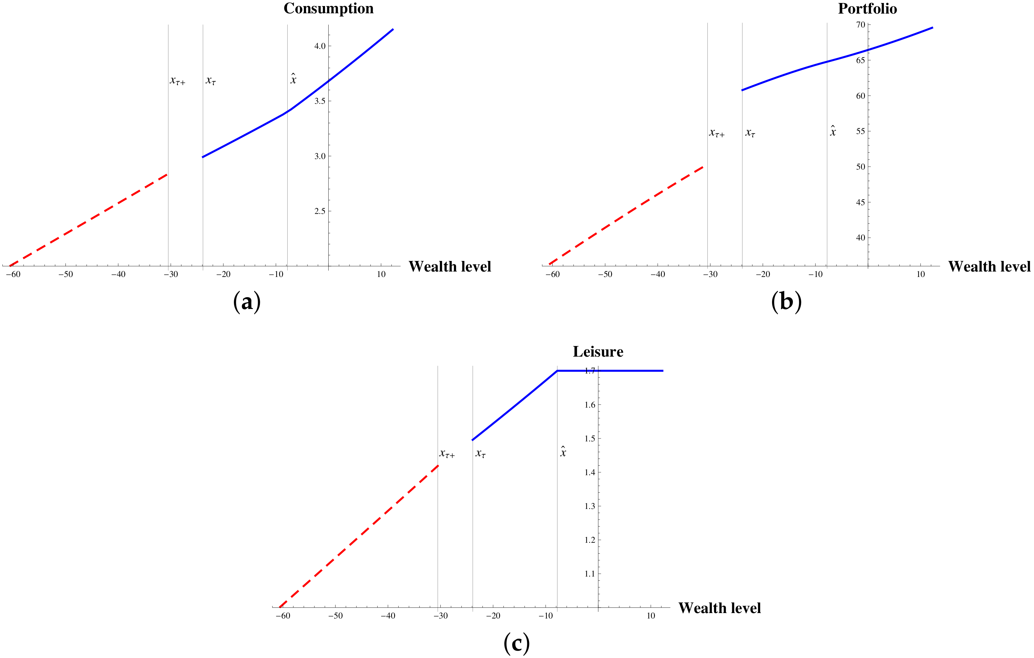
Figure 1 shows the optimal consumption, portfolio, and leisure for the debtor and filer. We see that consumption, portfolio, and leisure drop at bankruptcy. From Equation (17), the consumption drop at bankruptcy is given by

$${\overline{c}}_l-\overline{c}=({ϵ}^{\frac{1}{{\gamma }^{\ast }}}-1)\overline{c}<0,$$

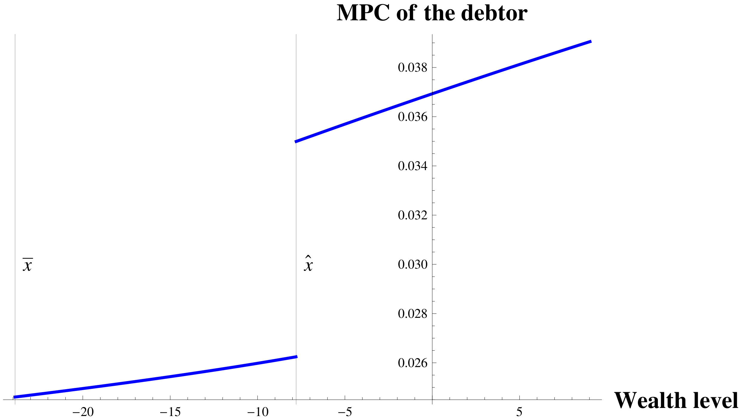
regardless of magnitude of the coefficient of relative risk aversion ${\gamma }^{\ast }$. To take a close look at the debtor’s consumption as the wealth level approaches the bankruptcy wealth level, we define the marginal propensity to consume (MPC) out of wealth as follows

$$MPC:=\frac{d{c}_t^{\ast }}{d{X}_t}.$$

From the inverse relation of $C_D^l(·)$ (resp. $C_D^L(·)$) and $X_D^l(·)$ (resp. $X_D^L(·)$), the MPC of the debtor is given by

$$\begin{array}{c}\hfill MPC=\left\{\begin{array}{cc}\frac{1}{\frac{d{X}_D^l\left(c\right)}{dc}{|}_{c=c_t^{\ast }}}\hfill & \overline{x}\le X_t<\widehat{x},\hfill \\ \frac{1}{\frac{d{X}_D^L\left(c\right)}{dc}{|}_{c=c_t^{\ast }}},\hfill & X_t\ge \widehat{x}.\hfill \end{array}\right.\end{array}$$

The optimal bankruptcy decision problem in this paper is similar to the optimal retirement problem (for example, [8,9,11]) in that both the optimal bankruptcy time and the retirement time are characterized as the first time the wealth level hit a certain threshold from above and below, respectively. From [11], which employ a Cobb-Douglas utility function, consumption jumps (resp. drops) at retirement if the coefficient of relative risk aversion is larger (resp. smaller) than 1. In addition, we see from [11] that the consumption is concave with wealth as the wealth level approaches to the retirement wealth level from below. On the other hand, we see from Figure 2 that when the debtor has an option to file for bankruptcy, consumption is convex with wealth as the wealth level approaches to the retirement wealth level from above.

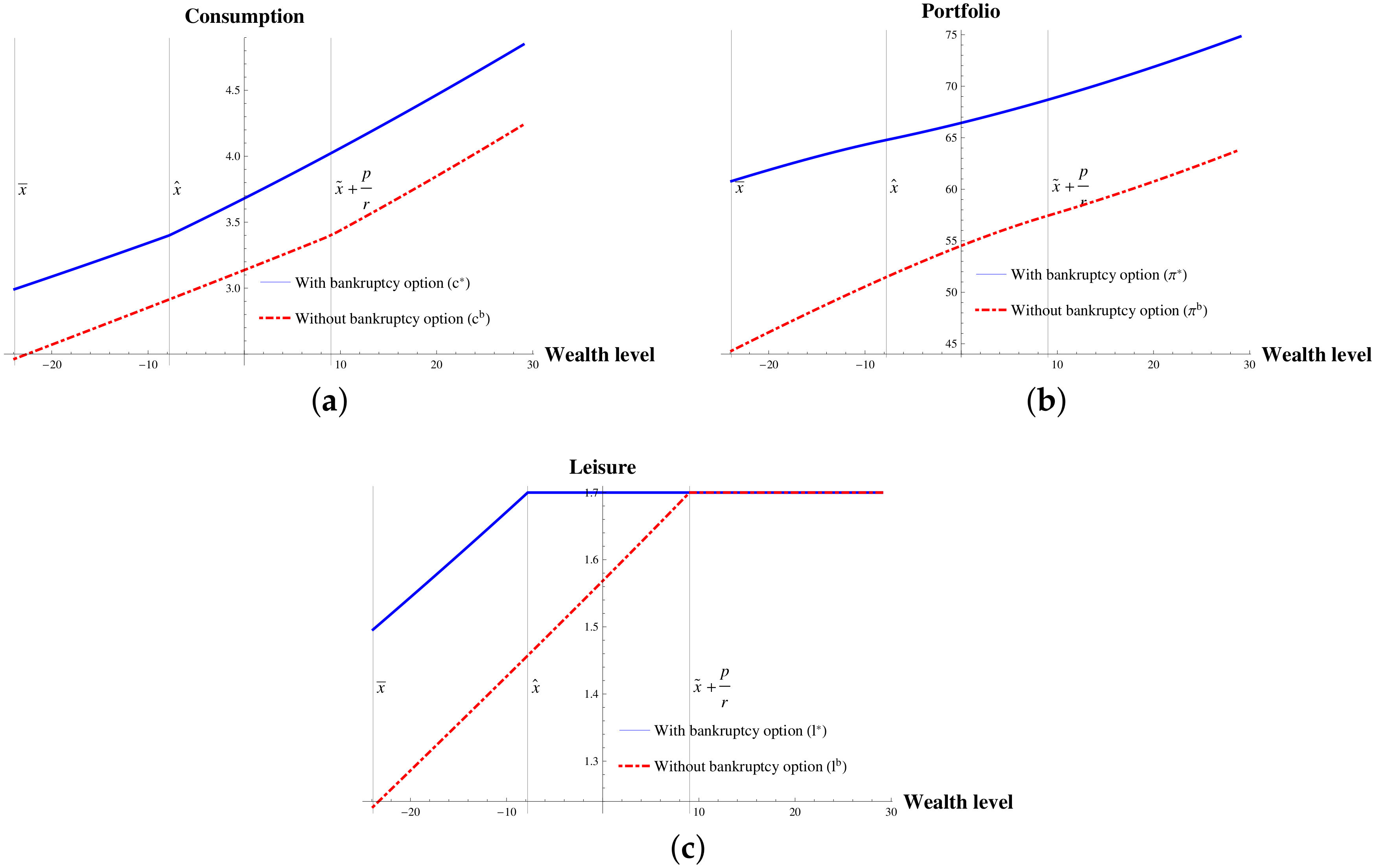
We compare the optimal strategies of a debtor who are given an opportunity to file for bankruptcy with those of a debtor without such an opportunity. Denote by $({\mathbf{c}}^b,{\mathbf{\pi }}^b,{\mathbf{l}}^b)$ the triple of the optimal consumption, portfolio, and leisure policies of a debtor without an option to file for bankruptcy. It is easy to find the optimal strategies $({\mathbf{c}}^b,{\mathbf{\pi }}^b,{\mathbf{l}}^b)$ which are given by

$$\begin{array}{c}\hfill \left\{\begin{array}{cc}{c}_t^b=C^l\left(X_t\right),\hfill & {\displaystyle -\frac{w\overline{L}-p}{r}\le X_t<\tilde{x}+\frac{p}{r},}\hfill \\ {\displaystyle {\pi }_t^b=\frac{\theta }{{\gamma }^{\ast }\sigma }\left\{-{\gamma }^{\ast }{m}_{-}A{C}^l{\left(X_t\right)}^{-{\gamma }^{\ast }{m}_{-}}+\frac{1}{\alpha K^{\ast }}{C}^l\left(X_t\right)\right\},}\hfill & {\displaystyle -\frac{w\overline{L}-p}{r}\le X_t<\tilde{x}+\frac{p}{r},}\hfill \\ {\displaystyle l_t^{\ast }={\left(\frac{w\alpha }{1-\alpha }\right)}^{-1}{C}^l\left(X_t\right),}\hfill & {\displaystyle -\frac{w\overline{L}-p}{r}\le X_t<\tilde{x}+\frac{p}{r},}\hfill \end{array}\right.\end{array}$$

$$\begin{array}{c}\hfill \left\{\begin{array}{cc}{c}_t^{\ast }=C^L\left(X_t\right),\hfill & {\displaystyle X_t\ge \tilde{x}+\frac{p}{r},}\hfill \\ {\displaystyle {\pi }_t^{\ast }=\frac{\theta }{\gamma \sigma }\left\{-\gamma m_{+}B{C}^L{\left(X_t\right)}^{-\gamma m_{+}}+\frac{1}{K}{C}^L\left(X_t\right)\right\},}\hfill & {\displaystyle X_t\ge \tilde{x}+\frac{p}{r},}\hfill \\ {\displaystyle l_t^{\ast }=L,}\hfill & {\displaystyle X_t\ge \tilde{x}+\frac{p}{r},}\hfill \end{array}\right.\end{array}$$

where $C^l(·)$ (resp. $C^L(·)$) is the inverse function of $X^l(·):=X_F^l(·)+p/r$ (resp. $X^L(·):=X_F^L(·)+p/r$).

From Figure 3, we see that an opportunity to file for bankruptcy leads a debtor to consume more and work less than he/she does without an option to file for bankruptcy. Due to the existence of a refuge from financial distress, a debtor with such an option can enjoy consumption and leisure more and reduces savings comparing to a debtor without and option to file for bankruptcy. Also, with an option to file for bankruptcy the debtor tends to invest more in the risky asset than he/she does without the option.

5. Conclusions

This paper investigates the optimal consumption, portfolio and leisure of a debtor who is eligible for Chapter 7 bankruptcy. Explicit expressions for the optimal strategies can be obtained with a Cobb-Douglas utility function. There exists consumption and leisure drops at bankruptcy regardless of magnitude of the coefficient of relative risk aversion. An option to file for bankruptcy enables the debtor to increase consumption, leisure and to invest more in the risky asset.

Unlike the debtor, we assume that the filer receives a fixed income stream and is not able to control labor supply. Due to the bankruptcy flag, the filer is likely to face restriction to borrow against future income, but we assume that the filer can borrow up the 100% of the present value of the future income stream. These are limitations to this study. Therefore, considering the liquidity constraint of the filer or providing labor supply flexibility to the filer, although methodologically challenging, can increase realism and are possible future research directions.

References

1. Buckley, F.H.; Brinig, M.F. The bankruptcy puzzle. J. Leg. Stud. 1998, 27, 187–207. [Google Scholar] [CrossRef] [Green Version]
2. White, M.J. Bankruptcy Reform and Credit Cards. J. Econ. Perspect. 2007, 21, 175–199. [Google Scholar] [CrossRef] [Green Version]
3. Dobbie, W.; Song, J. Debt Relief and Debtor Outcomes: Measuring the Effects of Consumer Bankruptcy Protection. Am. Econ. Rev. 2015, 105, 1272–1311. [Google Scholar] [CrossRef] [Green Version]
4. Mahoney, N. Bankruptcy as Implicit Health Insurance. Am. Econ. Rev. 2015, 105, 710–746. [Google Scholar] [CrossRef] [PubMed] [Green Version]
5. Filer, L.; Fisher, J.D. Do liquidity constraints generate excess sensitivity in consumption? New evidence from a sample of post-bankruptcy households. J. Macroecon. 2007, 29, 790–805. [Google Scholar] [CrossRef]
6. Han, S.; Li, G. Household Borrowing after Personal Bankruptcy. J. Money Credit. Bank. 2011, 43, 491–517. [Google Scholar] [CrossRef]
7. Livshits, I.; MacGee, J.; Tertilt, M. Consumer Bankruptcy: A Fresh Start. Am. Econ. Rev. 2007, 97, 402–418. [Google Scholar] [CrossRef] [Green Version]
8. Choi, K.J.; Shim, G. Disutility, Optimal Retirement, and Portfolio Selection. Math. Financ. 2006, 16, 443–467. [Google Scholar] [CrossRef]
9. Choi, K.J.; Shim, G.; Shin, Y.H. Optimal Portfolio, Consumption-Leisure and Retirement Choice Problem with CES Utility. Math. Financ. 2008, 18, 445–472. [Google Scholar] [CrossRef]
10. Dybvig, P.H.; Liu, H. Lifetime Consumption and Investment: Retirement and Constrained Borrowing. J. Econ. Theory 2010, 145, 885–907. [Google Scholar] [CrossRef] [Green Version]
11. Farhi, E.; Panageas, S. Saving and investing for early retirement: A theoretical analysis. J. Financ. Econ. 2007, 83, 87–121. [Google Scholar] [CrossRef]
12. Lee, H.S.; Jang, B. Retirement with risk aversion change and borrowing constraints. Financ. Res. Lett. 2016, 16, 112–124. [Google Scholar] [CrossRef]
13. Lim, B.H.; Shin, Y.H. Optimal Investment, Consumption and Retirement Decision with Disutility and Borrowing Constraints. Quant. Financ. 2011, 11, 1581–1592. [Google Scholar] [CrossRef]
14. Park, S.; Jang, B. Optimal Retirement Strategy with a Negative Wealth Constraint. Oper. Res. Lett. 2014, 42, 208–212. [Google Scholar] [CrossRef]
15. Jeanblanc, M.; Lakner, P.; Kadam, A. Optimal Bankruptcy Time and Consumption/Investment Policies on an Infinite Horizon with a Continuous Debt Repayment Until Bankruptcy. Math. Oper. Res. 2004, 29, 649–671. [Google Scholar] [CrossRef]
16. Lee, H.S.; Lim, B.H. Strategic Default and Post-Bankruptcy Liquidity Constraint; Working Paper; 2019; submitted. [Google Scholar]
17. Han, S.; Li, W. Fresh Start or Head Start? The Effects of Filing for Personal Bankruptcy on Work Effort. J. Financ. Serv. Res. 2007, 31, 123–152. [Google Scholar] [CrossRef]
18. Chen, D.; Zhao, J. The impact of personal bankruptcy on labor supply decisions. Rev. Econ. Dyn. 2017, 27, 40–61. [Google Scholar] [CrossRef]
19. Dobbie, W.; Goldsmith-Pinkham, P.; Yang, C.S. Consumer Bankruptcy and Financial Health. Rev. Econ. Stat. 2017, 99, 853–869. [Google Scholar] [CrossRef] [Green Version]
20. Karatzas, I.; Lehoczky, J.; Sethi, S.; Shreve, S.E. Explicit solution of a general consumption/investment problem. Math. Oper. Res. 1986, 11, 261–294. [Google Scholar] [CrossRef]
Figure 1. Debtor’s and Filer’s optimal strategies ( γ = 2 , r = 0.03 , μ = 0.07 , σ = 0.2 , β = 0.07 , α = 0.5 , w = 2 , L ¯ = 2 , L = 1.7 , p = 0.6 , ϵ = 0.9 , ν = 0.5 p / r ). (a) Consumption. (b) Porfolio. (c) Leisure.
Symmetry 12 00827 g001
Figure 2. MPC of the debtor ( γ = 2 , r = 0.03 , μ = 0.07 , σ = 0.2 , β = 0.07 , α = 0.5 , w = 2 , L ¯ = 2 , L = 1.7 , p = 0.6 , ϵ = 0.9 , ν = 0.5 p / r ).
Symmetry 12 00827 g002
Figure 3. Debtor’s optimal strategies with and without option to file for bankruptcy ( γ = 2 , r = 0.03 , μ = 0.07 , σ = 0.2 , β = 0.07 , α = 0.5 , w = 2 , L ¯ = 2 , L = 1.7 , p = 0.6 , ϵ = 0.9 , ν = 0.5 p / r ) (a) Consumption. (b) Porfolio. (c) Leisure.
Symmetry 12 00827 g003