Abstract
The fluctuation of the stock market has a symmetrical characteristic. To improve the performance of self-forecasting, it is crucial to summarize and accurately express internal fluctuation rules from the historical time series dataset. However, due to the influence of external interference factors, these internal rules are difficult to express by traditional mathematical models. In this paper, a novel forecasting model is proposed based on probabilistic linguistic logical relationships generated from historical time series dataset. The proposed model introduces linguistic variables with positive and negative symmetrical judgements to represent the direction of stock market fluctuation. Meanwhile, daily fluctuation trends of a stock market are represented by a probabilistic linguistic term set, which consist of daily status and its recent historical statuses. First, historical time series of a stock market is transformed into a fluctuation time series (FTS) by the first-order difference transformation. Then, a fuzzy linguistic variable is employed to represent each value in the fluctuation time series, according to predefined intervals. Next, left hand sides of fuzzy logical relationships between currents and their corresponding histories can be expressed by probabilistic linguistic term sets and similar ones can be grouped to generate probabilistic linguistic logical relationships. Lastly, based on the probabilistic linguistic term set expression of the current status and the corresponding historical statuses, distance measurement is employed to find the most proper probabilistic linguistic logical relationship for future forecasting. For the convenience of comparing the prediction performance of the model from the perspective of accuracy, this paper takes the closing price dataset of Taiwan Stock Exchange Capitalization Weighted Stock Index (TAIEX) as an example. Compared with the prediction results of previous studies, the proposed model has the advantages of stable prediction performance, simple model design, and an easy to understand platform. In order to test the performance of the model for other datasets, we use the prediction of the Shanghai Stock Exchange Composite Index (SHSECI) to prove its universality.
1. Introduction
Accurate predictions of future fluctuation for financial data can help investors hedge against risk. However, affected by high noise, instability, and long-term unpredictability of the stock market, it is difficult to predict the future trend of the stock market with absolute accuracy. Since each data set has its own inherent regulation of fluctuation, many researchers put forward many models that can predict the future by learning historical fluctuation laws, such as a regression analysis model [1], an autoregressive integrated moving average (ARIMA) model [2], an autoregressive conditional heteroscedasticity (ARCH) model [3], generalized ARCH (GARCH) [4], and more. These models use different methods to extract rules from historical data and employ them to predict the future. However, due to the interference of noise and random factors, over-fitting with historical data may lead to the lack of universality of rules, which makes the predicted results unsatisfactory.
Stock market fluctuation has symmetrical characteristics, which shows two aspects including the symmetry of fluctuation directions, the symmetry of historical fluctuation, and future trend. Affected by the dynamic external environment, the fluctuation of the financial time series dataset is a complicated nonlinear system with uncertainty, which makes it difficult to be expressed by traditional mathematical models. Inspired by Zadeh’s theory, Song and Chissom proposed fuzzy time series (FTS) prediction model [5,6,7] in 1993 to predict nonlinear complexed problems. The first fuzzy time series model was a first-order time-invariant FTS model for predicting enrollments of the university in the United States. Compared with traditional regressive models, the FTS model has many advantages because of its outstanding performance in expressing logical rules. Related models are also introduced to forecast project cost [8] and electricity load demand [9]. In a financial environment, the FTS method is widely used to predict stock index [10,11,12]. FTS-based models reduce the negative impact of random and uncertain factors on the prediction results by means of fuzziness, and the prediction accuracy is significantly improved when compared with the traditional regression method.
Fuzzy time series mainly consists of three parts: (1) interval division and fuzzification, (2) establishment of a fuzzy relationship, and (3) prediction and defuzzification. To state appropriate fuzzy logical relationships, fuzzy auto regressive (AR) models and fuzzy auto regressive and moving average (ARMA) models are widely adopted to show the impact of recurrence and weights in different fuzzy logical relationships [13,14,15,16,17,18,19]. With the development of computers, machine learning, and artificial intelligence, many scholars have even introduced neural networks and machine learning programs [19,20,21,22,23,24,25] to discover prediction rules from historical time series. In the forecasting process, the obtained logical relationships were used as rules. However, the FTS prediction model is based on the extraction rules of the first or multi-order continuous historical state, and the low-order model cannot fully reflect the periodic characteristics of the stock market fluctuation. At the same time, the high-order model will cause the lack of rules in the prediction stage due to the strict matching requirements of the fluctuation series.
In order to express the rules in time series more accurately and avoid the lack of rules, Guan et al. [26] introduced neutrosophic sets (NSs). NSs was proposed by Smarandache [27] from the philosophical thinking, which consisted of three degrees of truth, indeterminacy, and falsity. Many scholars have extended the application of the neutrosophic set to the field of disease diagnosis, prediction, and so on. In Guan’s model, historical states are mapped to the three dimensions of the neutrosophic set, and the matching of rules is realized by similarity, which avoids the problem of rules missing in the multi-order model. However, Guan’s model cannot reflect more detailed information such as fluctuation range because it maps the fluctuation states into only three dimensions.
Inspired by this, we introduce probabilistic linguistic terms set to express the fluctuation status and distance measurement to find the best matching rule. The probabilistic linguistic terms set was proposed by Pang et al. [28] in 2016. Each term was composed of corresponding probabilistic information, and Tang et al. [29] called it a probabilistic linguistic element. Linguistic variables in a probabilistic linguistic term set have positive and negative symmetrical judgements, which are employed to express different levels of decision direction. The probabilistic linguistic term set enriches decision makers’ way of expressing preference information and strengthens their ability of expressing uncertainty information. Probabilistic linguistic has been widely used in decision making [30,31,32,33,34], risk emergency plan decision making, and more. Probabilistic linguistics were successfully applied to decision making but rarely applied to forecasting problems.
This paper introduces probability linguistics into stock market prediction. A prediction model based on probabilistic linguistic theory and fuzzy logic relationship between current and historical states is proposed. For the initial step, the original time series of the stock market is represented as a fluctuation time series by calculating the difference between each piece of data with that of the previous day. The fluctuation time series is then fuzzified into a fuzzy-fluctuation time series. Next, probabilistic linguistic logical rules can be generated from traditional fuzzy logical relationships. Lastly, based on the probabilistic linguistic term set expression of current status and the corresponding historical statuses, distance measurement is employed to find the most proper probabilistic linguistic logical relationship for future forecasting. The advantages of this model lies in the following aspects. (1)The combination of the symmetrical characteristic of language variables and the symmetrical direction of the stock market fluctuation makes it convenient to describe the state and evolution trend of stock market fluctuation. Meanwhile, the fuzziness of language variables helps to reduce the interference of noise information. (2) Probabilistic linguistic logical rules can explore the internal rules of the actual existence of sequential data in an unsupervised fashion. (3) The probabilistic linguistic forecasting model can reasonably reduce the influence of noises from the internal rules by proper fuzzy treatment. The main contributions of this paper are as follows. (1) It introduced the probability linguistic method into the time series forecasting model, expanding the application field of this method. (2) The expression advantages of probability linguistics in uncertainty problems improve the reflection of the uncertainty of time series fluctuation. It provides a new expression form of fuzzy time series and deepens related research. (3) The distance measure function of probability language is used as the matching method of forecasting rules, which provides a new idea for future forecasting. The Taiwan Stock Exchange Capitalization Weighted Stock Index (TAIEX) data set from 1997 to 2005 and Shanghai Stock Exchange Composite Index (SHSECI) from 1998 to 2006 are taken as examples to verify the validation and universality of the proposed model. We also compare experimental results with some existing models to test the performance.
The second part introduces the basic concepts of fuzzy fluctuation time series and probability linguistic related theories. The third part introduces the prediction method based on probability linguistic logical rules. The fourth part uses the Taiwan Stock Exchange Capitalization Weighted Stock Index (TAIEX) data set from 1997 to 2005 and Shanghai Stock Exchange Composite Index (SHSECI) data from 2007 to 2015 to forecast the stock market. The fifth part summarizes the conclusions and potential problems in future research.
2. Preliminaries
2.1. Definition of Fuzzy-Fluctuation Time Series (FFTS)
Fuzzy time series was proposed by Song and Chissom [5,6,7]. In this section, we propose the concept of fuzzy-fluctuation time series (FFTS) based on existing Fuzzy time series.
Definition 1 (Linguistic Fuzzy Set).
Let U be a universe of discourse, then a fuzzy setin U can be defined by its membership function, , wheredenotes the grade of membership of, U =.
Let be a linguistic term set (LTS) describing the meaning of the fuzzy set with corresponding to For example, describes the fluctuation trends of a stock market. The element and its subscript are strictly monotonically increasing [35]. Therefore, the function can be defined by .
Definition 2 (Fuzzy-Fluctuation Time Series).
Letbe a time series of real numbers, where T is the number of the time series.can be defined by, whereis called fluctuation time series (FTS). Each element ofcan be represented by a linguistic fuzzy setas defined in Definition 1.is a fuzzy-fluctuation time series (FFTS) generated from the original.
Definition 3 (Fuzzy-Fluctuation Logical Relationship).
Letbe a FFTS. Assumeis determined by, then the fuzzy-fluctuation logical relationship is represented by:
It is called the nth-order fuzzy-fluctuation logical relationship (FFLR) of the fuzzy-fluctuation time series, where is called the left-hand side (LHS) and is called the right-hand side (RHS) of the FFLR.
2.2. Concept of Probabilistic Linguistic
In 2016, Pang et al. [28] proposed the theory of the probabilistic linguistic term set (PLTS).
Definition 4 (Probabilistic Linguistic Term Set).
Letbe a linguistic term set (LTS), a PLTS can be defined as:
whereis called a probabilistic linguistic variable (PLV), which is the linguistic termassociated with the probability.
Definition 5 (Conversion of Fuzzy Fluctuation Logical Relationship).
Letbe the LHS of a nth-order FFLR. It can be converted to a probabilistic linguistic term set (PLTS) as follows.
whereif the subscript of X(t − i) is equal toand 0, otherwise.is called the PLTS form of the LHS (PLHS) expression of a FFLR.
Example 1.
Let= 4 as defined in Definition 1. The LHS of a FFLRcan be converted to a probabilistic linguistic term set (PLTS). For convenience, the PLHS of the FFLR can be represented by the probability of each linguistic variable of an LTS in order. For example, the above PLTS can be simplified to be represented by.
Definition 6 (Probabilistic Linguistic Logical Relationship).
Letbe a FFTS, and L(t) is the PLHS expression of the FFTS. The RHSs of FFLRs with the same L(t) can be grouped by putting all their RHSs together as on the RHS of the FFLR, which can be converted a PLTSaccording to definition 5. By this way, a FFLR can be represented by a probabilistic linguistic logical relationship (PLLR) as
Example 2.
For a FFLR, all FFLRs with the same PLHSare as follows:, , ,, ,,,and. The RHSs of these FFLRs can be grouped to (, which can be represented by ). Thus, a PLLR can be generated as , which can be simplified to be represented by.
2.3. Distance Measurement
Definition 7 (Distance Measurement) [36].
Letandbe any two PLTSs. The generalized distance betweenandcan be defined as follows.
whereis the linguistic scale function, which can be defined as follows.
Evidently, if r = 1, then Equation (4) is reduced to the Hamming-Hausdorff distance and it is Euclidean-Hausdorff distance when r = 2.
2.4. Score Function
Definition 8 (Score of PLTS) [36].
Letbe a PLTS. The score functionofis defined as follows.
where m = .
Example 3.
For a PLTS, its score is calculated as:
3. A Novel Forecasting Model Based on Probabilistic Linguistics
Based on probabilistic linguistic logical relationships, a new forecasting model can be developed. In order to compare the forecasting results with existing works [11,22,37,38,39,40,41,42,43,44], the authentic TAXEI (Taiwan Stock Exchange Capitalization Weighted Stock Index) in 2004 is employed to illustrate the forecasting process. The dataset TAXEI in 2004 is split into two parts. The training dataset takes place from January 2004 to October 2004 and the testing dataset occurs from November 2004 to December 2004. The basic steps of the proposed model are shown in Figure 1.
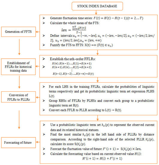
Figure 1.
Flowchart of the proposed forecasting model. FTS-fuzzy time series, FFLR–fuzzy fluctuation logical relationship, LHS-left hand side of FFLR, RHS–right hand side of FFLR, PLLR-probabilistic linguistic logical relationship, PLHS-left hand of PLLR, also the probabilistic linguistic term set(PLTS) format of a LHS.
Step 1. Generation of FFTS
For an original time series , its corresponding fluctuation time series is determined by . Let represent the whole mean of all elements in the fluctuation time series . Define intervals , and linguistic terms set . can be fuzzified into a fuzzy-fluctuation time series according to Definition 2.
Step 2. Establishment of FFLRs for Historical Training Data
According to Definition 3, each in the historical training dataset can establish FFLR with its related historical data as .
Step 3. Conversion of FFLRs to PLLRs
According to Definition 5, each LHS of FFLRs can be expressed by a PLHS L(t). Then, we can generate the for different respectively, as described in Definition 6. Thus, the FFLRs for the historical training dataset are converted into PLLRs.
Step 4. Forecasting of the Future
For each observed point in the test time series, use a to represent its current and related historical statuses. Then, find the most similar in the left-hand side of PLLRs generated in step 3 by distance comparison, as described in Definition 7. According to the right-hand side of the selected PLLR , calculate its score S( as described in Definition 8. The fluctuation value of the next point can be forecasted as . Lastly, the forecasting value can be calculated based on the observed point by .
4. Empirical Analysis
4.1. Forecasting of the Taiwan Stock Exchange Capitalization Weighted Stock Index
Many studies use TAIEX2004 as an example to illustrate their proposed forecasting methods [11,18,19,22,37,38,39,40,41,42,43,44]. In order to test the accuracy, we also use TAIEX2004 to illustrate the proposed method.
Step 1: Calculate the fluctuation value for each data in the historical training dataset of TAIEX2004. Then, calculate the whole mean of the fluctuation numbers of the training dataset for further fuzzification. In this case, the whole mean of the historical dataset of TAIEX2004 from January to October is = 61.87. Therefore, the historical training dataset can be represented by FFTS, as shown in Appendix Table A1.
Step 2: Build nth-order FFLRs according to the relationships of each data and its historical fluctuations (as shown in Appendix Table A2). For convenience, the element is simplified to number i in the expression of FFLRs.
Step 3: In order to convert the FFLRs to PLLRs, the LHSs of the FFLRs in Table A2 are converted to PLHSs. Then, the RHSs of the FFLRs are grouped by PLHSs and expressed by probabilistic linguistic terms sets. In this way, FFLRs are converted to PLLRs. For example, the LHS of FFLR can be represented by a probabilistic linguistic term set and simplified as . All RHSs with the same PLHS can be grouped to (, which can be further converted to a probabilistic linguistic term set and simplified as . Thus, a PLLR is generated. The detailed process is shown in Figure 2.
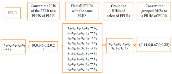
Figure 2.
Group and converting process from the fuzzy-fluctuation logical relationship (FFLR) to the probabilistic linguistic logical relationship (PLLR). FFLR-fuzzy-fluctuation logical relationship, LHS–left hand side of FFLR, RHS–right hand side of FFLR, PLLR-probabilistic linguistic logical relationship, PLHS-left hand of PLLR, PRHS-right hand of PLLR.

Table 1.
Probabilistic linguistic logical relationship (PLLR) for the historical training dataset of Taiwan Stock Exchange Capitalization Weighted Stock Index (TAIEX) 2004.
Step 4: Use the PLLRs obtained from the historical training dateset to forecast the testing dataset from 1 November 2004 to 31 December 2004. For example, set current point is the date 29 October 2004 and the forecasting date is 1 November 2004. First, the 5th-order current and related historical fuzzy-fluctuation trends are (as shown in Table A1 from date 29 October to 22 October), which can be represented by a probabilistic linguistic term set . Then, by using the distance measurement method described in Definition 8 (where the parameter r is set to 1), the most optimal PLLR is . Therefore, the fuzzified forecasting fluctuation can be obtained by the score of the RHS of PLLR.
It can be defuzzified by:
At last, the forecasted value can be calculated through the current value and the fluctuation value.
Table 2.
Forecasting results from 1 November 2004 to 31 December 2004.
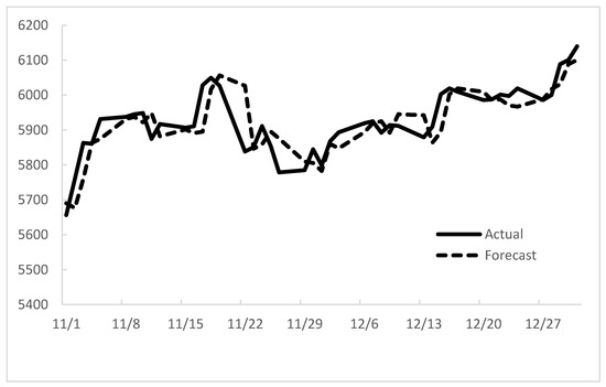
Figure 3.
Forecasting results from 1 November 2004 to 31 December 2004.
From the perspective of accuracy, a performance assessment can be carried out comparing forecasted values and the actual values. There are many indicators that have been verified to be useful for difference comparisons, such as the mean squared error (MSE), the root of the mean squared error (RMSE), the mean absolute error (MAE), and the mean percentage error (MPE). The definitions are described as follows.
where t = 1,2,…,n denotes the position of series to be compared, n denotes the number of the series, and forecast (t) and actual (t) denote the forecasted value and actual value at position t, respectively.
With respect to the proposed method for the 5th-order forecasting model, the mean squared error (MSE), the root of the mean squared error (RMSE), the mean absolute error (MAE), and the mean percentage error (MPE) are 3029.91, 55.04, 5927.36, 38.87, respectively. The forecasting errors of RMSE for different nth-order models are shown in Table 3.
Table 3.
Comparison of forecasting errors for different nth-order models.
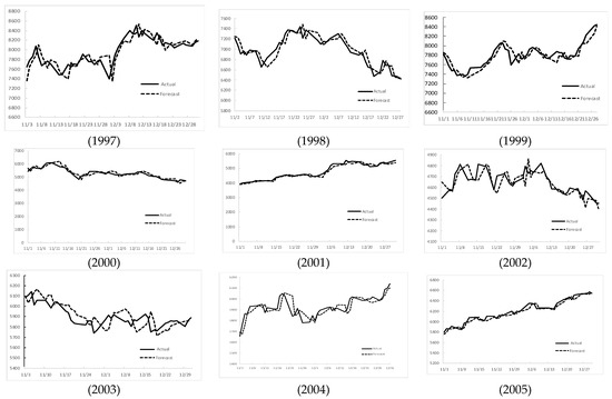
Figure 4.
The stock market fluctuation for the Taiwan Stock Exchange Capitalization Weighted Stock Index (TAIEX) test dataset (1997–2005).
Table 4.
Root mean square errors (RMSEs) of forecast errors for Taiwan Stock Exchange Capitalization Weighted Stock Index (TAIEX) 1997 to 2005.
Table 5 shows a comparison of the RMSEs of different methods for forecasting the TAIEX 1997–2005.
Table 5.
A comparison of RMSEs for forecasting TAIEX 1997–2005.
From Table 5, we can see that the performance of the method presented in this paper is stable and acceptable. Although performance of the proposed method is not the best method for all time series, its average performance is the best. In fact, accuracy is not the unique judgement criteria for a forecasting method. One particularly preferred aspect is that it can be easily realized by a computer because it does not need human intervention. Meanwhile, the introduction of a probabilistic linguistic term set makes it easy to understand and possible to employ a distance measurement method to find out the most appropriate rules for further forecasting. From that point of view, it has better universality for different types of time series.
4.2. Forecasting Shanghai Stock Exchange Composite Index
In order to verify the universality of the proposed model, the famous SHSECI (Shanghai Stock Exchange Composite Index) in China is also taken as an example. We carry out forecasting for the SHSECI from 2007 to 2015 by the proposed method. The realistic datasets for each year are also divided into the training dataset and testing dataset. The RMSEs of the forecasting results for SHSECI from 2007 to 2015 are shown in Table 6. It shows that the SHSECI stock market can be successfully forecasted by the proposed model.
Table 6.
RMSEs of forecasting results for the Shanghai Stock Exchange Composite Index (SHSECI) from 2007 to 2015.
5. Conclusions
Considering the symmetrical characteristics of stock market fluctuation, this paper proposes a novel forecasting model based on symmetrical linguistic variables. The proposed model extends traditional FFLRs to PLLRs. Through such a transformation, distance measurement between probabilistic linguistic term sets can be employed to optimize the expression of forecasting rules. The greatest aspect of the proposed method is that it can retain more detailed fluctuation information while reducing overfitting information. Meanwhile, the distance comparison fuction makes it easy to solve new situations and avoid a lack of rules. This makes it more universal when compared with traditional models. In addition, the definability of high order and linguistic terms makes it more flexible than many other methods. Compared with the prediction results of previous studies, the proposed model has the advantages of stable prediction performance, simple model design, and an easy to understand platform. The success of forecasting SHSECI verifies the universality of the proposed model.
This model uses the simplest form of probability linguistic variables to express the fuzzy fluctuation states of a time series. In a realistic stock market, there are a lot of disturbance factors concealing the internal fluctuation law of the time series. In order to reveal the internal fluctuation law, it is important to select a suitable method to retain the information reflecting the internal fluctuation law and to erase the influence of noise to a maximum extent. From this perspective, the selection of the fuzzification method needs to be deeply discussed. In this regard, the existing decision-making methods can provide useful information [45]. In the follow-up study, we can make full use of the latest research results in decision-making and further optimize the prediction method. At the same time, other external factors related to the fluctuation of the stock market will also be introduced to establish new models.
Author Contributions
Methodology, A.Z., conceptualization, A.Z., writing-original draft preparation, J.G., writing-review and editing, H.G. All authors have read and agreed to the published version of the manuscript.
Funding
This research was funded by major projects of the National Social Science Foundation of China under Grants grant number 19VHQ011.
Acknowledgments
The authors sincercely appreciate the comments and suggestions from anonymous reviewers, which improve the quality of this paper.
Conflicts of Interest
The authors declare no conflict of interest.
Appendix A
Table A1.
Fuzzy-Fluctuation Time Series (FFTS) from 2 January to 29 October for Taiwan Stock Exchange Capitalization Weighted Stock Index (TAIEX) 2004.
Table A1.
Fuzzy-Fluctuation Time Series (FFTS) from 2 January to 29 October for Taiwan Stock Exchange Capitalization Weighted Stock Index (TAIEX) 2004.
| Date (MM/DD/YY) | TAXEI | Fluctuation | Fuzzified | Date (MM/DD/YY) | TAXEI | Fluctuation | Fuzzified | Date (MM/DD/YY) | TAXEI | Fluctuation | Fuzzified |
|---|---|---|---|---|---|---|---|---|---|---|---|
| 01/02/04 | 6041.56 | - | - | 04/23/04 | 6748.1 | 16.01 | 2 | 08/06/04 | 5399.16 | −28.45 | 2 |
| 01/05/04 | 6125.42 | 83.86 | 4 | 04/26/04 | 6710.7 | −37.4 | 1 | 08/09/04 | 5399.45 | 0.29 | 2 |
| 01/06/04 | 6144.01 | 18.59 | 2 | 04/27/04 | 6646.8 | −63.9 | 0 | 08/10/04 | 5393.73 | −5.72 | 2 |
| 01/07/04 | 6141.25 | −2.76 | 2 | 04/28/04 | 6574.75 | −72.05 | 0 | 08/11/04 | 5367.34 | −26.39 | 2 |
| 01/08/04 | 6169.17 | 27.92 | 2 | 04/29/04 | 6402.21 | −172.54 | 0 | 08/12/04 | 5368.02 | 0.68 | 2 |
| 01/09/04 | 6226.98 | 57.81 | 3 | 04/30/04 | 6117.81 | −284.4 | 0 | 08/13/04 | 5389.93 | 21.91 | 2 |
| 01/12/04 | 6219.71 | −7.27 | 2 | 05/03/04 | 6029.77 | −88.04 | 0 | 08/16/04 | 5352.01 | −37.92 | 1 |
| 01/13/04 | 6210.22 | −9.49 | 2 | 05/04/04 | 6188.15 | 158.38 | 4 | 08/17/04 | 5342.49 | −9.52 | 2 |
| 01/14/04 | 6274.97 | 64.75 | 4 | 05/05/04 | 5854.23 | −333.92 | 0 | 08/18/04 | 5427.75 | 85.26 | 4 |
| 01/15/04 | 6264.37 | −10.6 | 2 | 05/06/04 | 5909.79 | 55.56 | 3 | 08/19/04 | 5602.99 | 175.24 | 4 |
| 01/16/04 | 6269.71 | 5.34 | 2 | 05/07/04 | 6040.26 | 130.47 | 4 | 08/20/04 | 5622.86 | 19.87 | 2 |
| 01/27/04 | 6384.63 | 114.92 | 4 | 05/10/04 | 5825.05 | −215.21 | 0 | 08/23/04 | 5660.97 | 38.11 | 3 |
| 01/28/04 | 6386.25 | 1.62 | 2 | 05/11/04 | 5886.36 | 61.31 | 4 | 08/26/04 | 5813.39 | 152.42 | 4 |
| 01/29/04 | 6312.65 | −73.6 | 0 | 05/12/04 | 5958.79 | 72.43 | 4 | 08/27/04 | 5797.71 | −15.68 | 2 |
| 01/30/04 | 6375.38 | 62.73 | 4 | 05/13/04 | 5918.09 | −40.7 | 1 | 08/30/04 | 5788.94 | −8.77 | 2 |
| 02/02/04 | 6319.96 | −55.42 | 1 | 05/14/04 | 5777.32 | −140.77 | 0 | 08/31/04 | 5765.54 | −23.4 | 2 |
| 02/03/04 | 6252.23 | −67.73 | 0 | 05/17/04 | 5482.96 | −294.36 | 0 | 09/01/04 | 5858.14 | 92.6 | 4 |
| 02/04/04 | 6241.39 | −10.84 | 2 | 05/18/04 | 5557.68 | 74.72 | 4 | 09/02/04 | 5852.85 | −5.29 | 2 |
| 02/05/04 | 6268.14 | 26.75 | 2 | 05/19/04 | 5860.58 | 302.9 | 4 | 09/03/04 | 5761.14 | −91.71 | 0 |
| 02/06/04 | 6353.35 | 85.21 | 4 | 05/20/04 | 5815.33 | −45.25 | 1 | 09/06/04 | 5775.99 | 14.85 | 2 |
| 02/09/04 | 6463.09 | 109.74 | 4 | 05/21/04 | 5964.94 | 149.61 | 4 | 09/07/04 | 5846.83 | 70.84 | 4 |
| 02/10/04 | 6488.34 | 25.25 | 2 | 05/24/04 | 5942.08 | −22.86 | 2 | 09/08/04 | 5846.02 | −0.81 | 2 |
| 02/11/04 | 6454.39 | −33.95 | 1 | 05/25/04 | 5958.38 | 16.3 | 2 | 09/09/04 | 5842.93 | −3.09 | 2 |
| 02/12/04 | 6436.95 | −17.44 | 2 | 05/26/04 | 6027.27 | 68.89 | 4 | 09/10/04 | 5846.19 | 3.26 | 2 |
| 02/13/04 | 6549.18 | 112.23 | 4 | 05/27/04 | 6033.05 | 5.78 | 2 | 09/13/04 | 5928.22 | 82.03 | 4 |
| 02/16/04 | 6565.37 | 16.19 | 2 | 05/28/04 | 6137.26 | 104.21 | 4 | 09/14/04 | 5919.77 | −8.45 | 2 |
| 02/17/04 | 6600.47 | 35.1 | 3 | 05/31/04 | 5977.84 | −159.42 | 0 | 09/15/04 | 5871.07 | −48.7 | 1 |
| 02/18/04 | 6605.85 | 5.38 | 2 | 06/01/04 | 5986.2 | 8.36 | 2 | 09/16/04 | 5891.05 | 19.98 | 2 |
| 02/19/04 | 6681.52 | 75.67 | 4 | 06/02/04 | 5875.67 | −110.53 | 0 | 09/17/04 | 5818.39 | −72.66 | 0 |
| 02/20/04 | 6665.54 | −15.98 | 2 | 06/03/04 | 5671.45 | −204.22 | 0 | 09/20/04 | 5864.54 | 46.15 | 3 |
| 02/23/04 | 6665.89 | 0.35 | 2 | 06/04/04 | 5724.89 | 53.44 | 3 | 09/21/04 | 5949.26 | 84.72 | 4 |
| 02/24/04 | 6589.23 | −76.66 | 0 | 06/07/04 | 5935.82 | 210.93 | 4 | 09/22/04 | 5970.18 | 20.92 | 2 |
| 02/25/04 | 6644.28 | 55.05 | 3 | 06/08/04 | 5986.76 | 50.94 | 3 | 09/23/04 | 5937.25 | −32.93 | 1 |
| 02/26/04 | 6693.25 | 48.97 | 3 | 06/09/04 | 5965.7 | −21.06 | 2 | 09/24/04 | 5892.21 | −45.04 | 1 |
| 02/27/04 | 6750.54 | 57.29 | 3 | 06/10/04 | 5867.51 | −98.19 | 0 | 09/27/04 | 5849.22 | −42.99 | 1 |
| 03/01/04 | 6888.43 | 137.89 | 4 | 06/11/04 | 5735.07 | −132.44 | 0 | 09/29/04 | 5809.75 | −39.47 | 1 |
| 03/02/04 | 6975.26 | 86.83 | 4 | 06/14/04 | 5574.08 | −160.99 | 0 | 09/30/04 | 5845.69 | 35.94 | 3 |
| 03/03/04 | 6932.17 | −43.09 | 1 | 06/15/04 | 5646.49 | 72.41 | 4 | 10/01/04 | 5945.35 | 99.66 | 4 |
| 03/04/04 | 7034.1 | 101.93 | 4 | 06/16/04 | 5560.16 | −86.33 | 0 | 10/04/04 | 6077.96 | 132.61 | 4 |
| 03/05/04 | 6943.68 | −90.42 | 0 | 06/17/04 | 5664.35 | 104.19 | 4 | 10/05/04 | 6081.01 | 3.05 | 2 |
| 03/08/04 | 6901.48 | −42.2 | 1 | 06/18/04 | 5569.29 | −95.06 | 0 | 10/06/04 | 6060.61 | −20.4 | 2 |
| 03/09/04 | 6973.9 | 72.42 | 4 | 06/21/04 | 5556.54 | −12.75 | 2 | 10/07/04 | 6103 | 42.39 | 3 |
| 03/10/04 | 6874.91 | −98.99 | 0 | 06/23/04 | 5729.3 | 172.76 | 4 | 10/08/04 | 6102.16 | −0.84 | 2 |
| 03/11/04 | 6879.11 | 4.2 | 2 | 06/24/04 | 5779.09 | 49.79 | 3 | 10/11/04 | 6089.28 | −12.88 | 2 |
| 03/12/04 | 6800.24 | −78.87 | 0 | 06/25/04 | 5802.55 | 23.46 | 2 | 10/12/04 | 5979.56 | −109.72 | 0 |
| 03/15/04 | 6635.98 | −164.26 | 0 | 06/28/04 | 5709.84 | −92.71 | 0 | 10/13/04 | 5963.07 | −16.49 | 2 |
| 03/16/04 | 6589.72 | −46.26 | 1 | 06/29/04 | 5741.52 | 31.68 | 3 | 10/14/04 | 5831.07 | −132 | 0 |
| 03/17/04 | 6577.98 | −11.74 | 2 | 06/30/04 | 5839.44 | 97.92 | 4 | 10/15/04 | 5820.82 | −10.25 | 2 |
| 03/18/04 | 6787.03 | 209.05 | 4 | 07/01/04 | 5836.91 | −2.53 | 2 | 10/18/04 | 5772.12 | −48.7 | 1 |
| 03/19/04 | 6815.09 | 28.06 | 2 | 07/02/04 | 5746.7 | −90.21 | 0 | 10/19/04 | 5807.79 | 35.67 | 3 |
| 03/22/04 | 6359.92 | −455.17 | 0 | 07/05/04 | 5659.78 | −86.92 | 0 | 10/20/04 | 5788.34 | −19.45 | 2 |
| 03/23/04 | 6172.89 | −187.03 | 0 | 07/06/04 | 5733.57 | 73.79 | 4 | 10/21/04 | 5797.24 | 8.9 | 2 |
| 03/24/04 | 6213.56 | 40.67 | 3 | 07/07/04 | 5727.78 | −5.79 | 2 | 10/22/04 | 5774.67 | −22.57 | 2 |
| 03/25/04 | 6156.73 | −56.83 | 1 | 07/08/04 | 5713.39 | −14.39 | 2 | 10/26/04 | 5662.88 | −111.79 | 0 |
| 03/26/04 | 6132.62 | −24.11 | 2 | 07/09/04 | 5777.72 | 64.33 | 4 | 10/27/04 | 5650.97 | −11.91 | 2 |
| 03/29/04 | 6474.11 | 341.49 | 4 | 07/12/04 | 5758.74 | −18.98 | 2 | 10/28/04 | 5695.56 | 44.59 | 3 |
| 03/30/04 | 6494.71 | 20.6 | 2 | 07/13/04 | 5685.57 | −73.17 | 0 | 10/29/04 | 5705.93 | 10.37 | 2 |
| 03/31/04 | 6522.19 | 27.48 | 2 | 07/14/04 | 5623.65 | −61.92 | 0 | ||||
| 04/01/04 | 6523.49 | 1.3 | 2 | 07/15/04 | 5542.8 | −80.85 | 0 | ||||
| 04/02/04 | 6545.54 | 22.05 | 2 | 07/16/04 | 5502.14 | −40.66 | 1 | ||||
| 04/05/04 | 6682.73 | 137.19 | 4 | 07/19/04 | 5489.1 | −13.04 | 2 | ||||
| 04/06/04 | 6635.54 | −47.19 | 1 | 07/20/04 | 5325.68 | −163.42 | 0 | ||||
| 04/07/04 | 6646.74 | 11.2 | 2 | 07/21/04 | 5409.13 | 83.45 | 4 | ||||
| 04/08/04 | 6672.86 | 26.12 | 2 | 07/22/04 | 5387.96 | −21.17 | 2 | ||||
| 04/09/04 | 6620.36 | −52.5 | 1 | 07/23/04 | 5373.85 | −14.11 | 2 | ||||
| 04/12/04 | 6777.78 | 157.42 | 4 | 07/26/04 | 5331.71 | −42.14 | 1 | ||||
| 04/13/04 | 6794.33 | 16.55 | 2 | 07/27/04 | 5398.61 | 66.9 | 4 | ||||
| 04/14/04 | 6880.18 | 85.85 | 4 | 07/28/04 | 5383.57 | −15.04 | 2 | ||||
| 04/15/04 | 6736.79 | −143.39 | 0 | 07/29/04 | 5349.66 | −33.91 | 1 | ||||
| 04/16/04 | 6818.2 | 81.41 | 4 | 07/30/04 | 5420.57 | 70.91 | 4 | ||||
| 04/19/04 | 6779.18 | −39.02 | 1 | 08/02/04 | 5350.4 | −70.17 | 0 | ||||
| 04/20/04 | 6799.97 | 20.79 | 2 | 08/03/04 | 5367.22 | 16.82 | 2 | ||||
| 04/21/04 | 6810.25 | 10.28 | 2 | 08/04/04 | 5316.87 | −50.35 | 1 | ||||
| 04/22/04 | 6732.09 | −78.16 | 0 | 08/05/04 | 5427.61 | 110.74 | 4 |
Table A2.
The fuzzy-fluctuation logical relationship (FFLRs) and the converted probabilitics linguistic term set form of the left hand side (PLHSs) of FFLRs for training data of TAIEX2004.
Table A2.
The fuzzy-fluctuation logical relationship (FFLRs) and the converted probabilitics linguistic term set form of the left hand side (PLHSs) of FFLRs for training data of TAIEX2004.
| Date (MM/DD/YY) | FFLR | PLHS | Date (MM/DD/YY) | FFLR | PLHS | Date (MM/DD/YY) | FFLR | PLHS | Date (MM/DD/YY) | FFLR | PLHS |
|---|---|---|---|---|---|---|---|---|---|---|---|
| 01/12/04 | (3,2,2,2,4)→2 | (0,0,0.6,0.2,0.2) | 03/30/04 | (4,2,1,3,0)→2 | (0.2,0.2,0.2,0.2,0.2) | 06/08/04 | (4,3,0,0,2)→3 | (0.4,0,0.2,0.2,0.2) | 08/18/04 | (2,1,2,2,2)→4 | (0,0.2,0.8,0,0) |
| 01/13/04 | (2,3,2,2,2)→2 | (0,0,0.8,0.2,0) | 03/31/04 | (2,4,2,1,3)→2 | (0,0.2,0.4,0.2,0.2) | 06/09/04 | (3,4,3,0,0)→2 | (0.4,0,0,0.4,0.2) | 08/19/04 | (4,2,1,2,2)→4 | (0,0.2,0.6,0,0.2) |
| 01/14/04 | (2,2,3,2,2)→4 | (0,0,0.8,0.2,0) | 04/01/04 | (2,2,4,2,1)→2 | (0,0.2,0.6,0,0.2) | 06/10/04 | (2,3,4,3,0)→0 | (0.2,0,0.2,0.4,0.2) | 08/20/04 | (4,4,2,1,2)→2 | (0,0.2,0.4,0,0.4) |
| 01/15/04 | (4,2,2,3,2)→2 | (0,0,0.6,0.2,0.2) | 04/02/04 | (2,2,2,4,2)→2 | (0,0,0.8,0,0.2) | 06/11/04 | (0,2,3,4,3)→0 | (0.2,0,0.2,0.4,0.2) | 08/23/04 | (2,4,4,2,1)→3 | (0,0.2,0.4,0,0.4) |
| 01/16/04 | (2,4,2,2,3)→2 | (0,0,0.6,0.2,0.2) | 04/05/04 | (2,2,2,2,4)→4 | (0,0,0.8,0,0.2) | 06/14/04 | (0,0,2,3,4)→0 | (0.4,0,0.2,0.2,0.2) | 08/26/04 | (3,2,4,4,2)→4 | (0,0,0.4,0.2,0.4) |
| 01/27/04 | (2,2,4,2,2)→4 | (0,0,0.8,0,0.2) | 04/06/04 | (4,2,2,2,2)→1 | (0,0,0.8,0,0.2) | 06/15/04 | (0,0,0,2,3)→4 | (0.6,0,0.2,0.2,0) | 08/27/04 | (4,3,2,4,4)→2 | (0,0,0.2,0.2,0.6) |
| 01/28/04 | (4,2,2,4,2)→2 | (0,0,0.6,0,0.4) | 04/07/04 | (1,4,2,2,2)→2 | (0,0.2,0.6,0,0.2) | 06/16/04 | (4,0,0,0,2)→0 | (0.6,0,0.2,0,0.2) | 08/30/04 | (2,4,3,2,4)→2 | (0,0,0.4,0.2,0.4) |
| 01/29/04 | (2,4,2,2,4)→0 | (0,0,0.6,0,0.4) | 04/08/04 | (2,1,4,2,2)→2 | (0,0.2,0.6,0,0.2) | 06/17/04 | (0,4,0,0,0)→4 | (0.8,0,0,0,0.2) | 08/31/04 | (2,2,4,3,2)→2 | (0,0,0.6,0.2,0.2) |
| 01/30/04 | (0,2,4,2,2)→4 | (0.2,0,0.6,0,0.2) | 04/09/04 | (2,2,1,4,2)→1 | (0,0.2,0.6,0,0.2) | 06/18/04 | (4,0,4,0,0)→0 | (0.6,0,0,0,0.4) | 09/01/04 | (2,2,2,4,3)→4 | (0,0,0.6,0.2,0.2) |
| 02/02/04 | (4,0,2,4,2)→1 | (0.2,0,0.4,0,0.4) | 04/12/04 | (1,2,2,1,4)→4 | (0,0.4,0.4,0,0.2) | 06/21/04 | (0,4,0,4,0)→2 | (0.6,0,0,0,0.4) | 09/02/04 | (4,2,2,2,4)→2 | (0,0,0.6,0,0.4) |
| 02/03/04 | (1,4,0,2,4)→0 | (0.2,0.2,0.2,0,0.4) | 04/13/04 | (4,1,2,2,1)→2 | (0,0.4,0.4,0,0.2) | 06/23/04 | (2,0,4,0,4)→4 | (0.4,0,0.2,0,0.4) | 09/03/04 | (2,4,2,2,2)→0 | (0,0,0.8,0,0.2) |
| 02/04/04 | (0,1,4,0,2)→2 | (0.4,0.2,0.2,0,0.2) | 04/14/04 | (2,4,1,2,2)→4 | (0,0.2,0.6,0,0.2) | 06/24/04 | (4,2,0,4,0)→3 | (0.4,0,0.2,0,0.4) | 09/06/04 | (0,2,4,2,2)→2 | (0.2,0,0.6,0,0.2) |
| 02/05/04 | (2,0,1,4,0)→2 | (0.4,0.2,0.2,0,0.2) | 04/15/04 | (4,2,4,1,2)→0 | (0,0.2,0.4,0,0.4) | 06/25/04 | (3,4,2,0,4)→2 | (0.2,0,0.2,0.2,0.4) | 09/07/04 | (2,0,2,4,2)→4 | (0.2,0,0.6,0,0.2) |
| 02/06/04 | (2,2,0,1,4)→4 | (0.2,0.2,0.4,0,0.2) | 04/16/04 | (0,4,2,4,1)→4 | (0.2,0.2,0.2,0,0.4) | 06/28/04 | (2,3,4,2,0)→0 | (0.2,0,0.4,0.2,0.2) | 09/08/04 | (4,2,0,2,4)→2 | (0.2,0,0.4,0,0.4) |
| 02/09/04 | (4,2,2,0,1)→4 | (0.2,0.2,0.4,0,0.2) | 04/19/04 | (4,0,4,2,4)→1 | (0.2,0,0.2,0,0.6) | 06/29/04 | (0,2,3,4,2)→3 | (0.2,0,0.4,0.2,0.2) | 09/09/04 | (2,4,2,0,2)→2 | (0.2,0,0.6,0,0.2) |
| 02/10/04 | (4,4,2,2,0)→2 | (0.2,0,0.4,0,0.4) | 04/20/04 | (1,4,0,4,2)→2 | (0.2,0.2,0.2,0,0.4) | 06/30/04 | (3,0,2,3,4)→4 | (0.2,0,0.2,0.4,0.2) | 09/10/04 | (2,2,4,2,0)→2 | (0.2,0,0.6,0,0.2) |
| 02/11/04 | (2,4,4,2,2)→1 | (0,0,0.6,0,0.4) | 04/21/04 | (2,1,4,0,4)→2 | (0.2,0.2,0.2,0,0.4) | 07/01/04 | (4,3,0,2,3)→2 | (0.2,0,0.2,0.4,0.2) | 09/13/04 | (2,2,2,4,2)→4 | (0,0,0.8,0,0.2) |
| 02/12/04 | (1,2,4,4,2)→2 | (0,0.2,0.4,0,0.4) | 04/22/04 | (2,2,1,4,0)→0 | (0.2,0.2,0.4,0,0.2) | 07/02/04 | (2,4,3,0,2)→0 | (0.2,0,0.4,0.2,0.2) | 09/14/04 | (4,2,2,2,4)→2 | (0,0,0.6,0,0.4) |
| 02/13/04 | (2,1,2,4,4)→4 | (0,0.2,0.4,0,0.4) | 04/23/04 | (0,2,2,1,4)→2 | (0.2,0.2,0.4,0,0.2) | 07/05/04 | (0,2,4,3,0)→0 | (0.4,0,0.2,0.2,0.2) | 09/15/04 | (2,4,2,2,2)→1 | (0,0,0.8,0,0.2) |
| 02/16/04 | (4,2,1,2,4)→2 | (0,0.2,0.4,0,0.4) | 04/26/04 | (2,0,2,2,1)→1 | (0.2,0.2,0.6,0,0) | 07/06/04 | (0,0,2,4,3)→4 | (0.4,0,0.2,0.2,0.2) | 09/16/04 | (1,2,4,2,2)→2 | (0,0.2,0.6,0,0.2) |
| 02/17/04 | (2,4,2,1,2)→3 | (0,0.2,0.6,0,0.2) | 04/27/04 | (1,2,0,2,2)→0 | (0.2,0.2,0.6,0,0) | 07/07/04 | (4,0,0,2,4)→2 | (0.4,0,0.2,0,0.4) | 09/17/04 | (2,1,2,4,2)→0 | (0,0.2,0.6,0,0.2) |
| 02/18/04 | (3,2,4,2,1)→2 | (0,0.2,0.4,0.2,0.2) | 04/28/04 | (0,1,2,0,2)→0 | (0.4,0.2,0.4,0,0) | 07/08/04 | (2,4,0,0,2)→2 | (0.4,0,0.4,0,0.2) | 09/20/04 | (0,2,1,2,4)→3 | (0.2,0.2,0.4,0,0.2) |
| 02/19/04 | (2,3,2,4,2)→4 | (0,0,0.6,0.2,0.2) | 04/29/04 | (0,0,1,2,0)→0 | (0.6,0.2,0.2,0,0) | 07/09/04 | (2,2,4,0,0)→4 | (0.4,0,0.4,0,0.2) | 09/21/04 | (3,0,2,1,2)→4 | (0.2,0.2,0.4,0.2,0) |
| 02/20/04 | (4,2,3,2,4)→2 | (0,0,0.4,0.2,0.4) | 04/30/04 | (0,0,0,1,2)→0 | (0.6,0.2,0.2,0,0) | 07/12/04 | (4,2,2,4,0)→2 | (0.2,0,0.4,0,0.4) | 09/22/04 | (4,3,0,2,1)→2 | (0.2,0.2,0.2,0.2,0.2) |
| 02/23/04 | (2,4,2,3,2)→2 | (0,0,0.6,0.2,0.2) | 05/03/04 | (0,0,0,0,1)→0 | (0.8,0.2,0,0,0) | 07/13/04 | (2,4,2,2,4)→0 | (0,0,0.6,0,0.4) | 09/23/04 | (2,4,3,0,2)→1 | (0.2,0,0.4,0.2,0.2) |
| 02/24/04 | (2,2,4,2,3)→0 | (0,0,0.6,0.2,0.2) | 05/04/04 | (0,0,0,0,0)→4 | (1,0,0,0,0) | 07/14/04 | (0,2,4,2,2)→0 | (0.2,0,0.6,0,0.2) | 09/24/04 | (1,2,4,3,0)→1 | (0.2,0.2,0.2,0.2,0.2) |
| 02/19/04 | (2,3,2,4,2)→4 | (0,0,0.6,0.2,0.2) | 04/29/04 | (0,0,1,2,0)→0 | (0.6,0.2,0.2,0,0) | 07/09/04 | (2,2,4,0,0)→4 | (0.4,0,0.4,0,0.2) | 09/21/04 | (3,0,2,1,2)→4 | (0.2,0.2,0.4,0.2,0) |
| 02/25/04 | (0,2,2,4,2)→3 | (0.2,0,0.6,0,0.2) | 05/05/04 | (4,0,0,0,0)→0 | (0.8,0,0,0,0.2) | 07/15/04 | (0,0,2,4,2)→0 | (0.4,0,0.4,0,0.2) | 09/27/04 | (1,1,2,4,3)→1 | (0,0.4,0.2,0.2,0.2) |
| 02/26/04 | (3,0,2,2,4)→3 | (0.2,0,0.4,0.2,0.2) | 05/06/04 | (0,4,0,0,0)→3 | (0.8,0,0,0,0.2) | 07/16/04 | (0,0,0,2,4)→1 | (0.6,0,0.2,0,0.2) | 09/29/04 | (1,1,1,2,4)→1 | (0,0.6,0.2,0,0.2) |
| 02/27/04 | (3,3,0,2,2)→3 | (0.2,0,0.4,0.4,0) | 05/07/04 | (3,0,4,0,0)→4 | (0.6,0,0,0.2,0.2) | 07/19/04 | (1,0,0,0,2)→2 | (0.6,0.2,0.2,0,0) | 09/30/04 | (1,1,1,1,2)→3 | (0,0.8,0.2,0,0) |
| 03/01/04 | (3,3,3,0,2)→4 | (0.2,0,0.2,0.6,0) | 05/10/04 | (4,3,0,4,0)→0 | (0.4,0,0,0.2,0.4) | 07/20/04 | (2,1,0,0,0)→0 | (0.6,0.2,0.2,0,0) | 10/01/04 | (3,1,1,1,1)→4 | (0,0.8,0,0.2,0) |
| 03/02/04 | (4,3,3,3,0)→4 | (0.2,0,0,0.6,0.2) | 05/11/04 | (0,4,3,0,4)→3 | (0.4,0,0,0.2,0.4) | 07/21/04 | (0,2,1,0,0)→4 | (0.6,0.2,0.2,0,0) | 10/04/04 | (4,3,1,1,1)→4 | (0,0.6,0,0.2,0.2) |
| 03/03/04 | (4,4,3,3,3)→1 | (0,0,0,0.6,0.4) | 05/12/04 | (3,0,4,3,0)→4 | (0.4,0,0,0.4,0.2) | 07/22/04 | (4,0,2,1,0)→2 | (0.4,0.2,0.2,0,0.2) | 10/05/04 | (4,4,3,1,1)→2 | (0,0.4,0,0.2,0.4) |
| 03/04/04 | (1,4,4,3,3)→4 | (0,0.2,0,0.4,0.4) | 05/13/04 | (4,3,0,4,3)→1 | (0.2,0,0,0.4,0.4) | 07/23/04 | (2,4,0,2,1)→2 | (0.2,0.2,0.4,0,0.2) | 10/06/04 | (2,4,4,3,1)→2 | (0,0.2,0.2,0.2,0.4) |
| 03/05/04 | (4,1,4,4,3)→0 | (0,0.2,0,0.2,0.6) | 05/14/04 | (1,4,3,0,4)→0 | (0.2,0.2,0,0.2,0.4) | 07/26/04 | (2,2,4,0,2)→1 | (0.2,0,0.6,0,0.2) | 10/07/04 | (2,2,4,4,3)→3 | (0,0,0.4,0.2,0.4) |
| 03/08/04 | (0,4,1,4,4)→1 | (0.2,0.2,0,0,0.6) | 05/17/04 | (0,1,4,3,0)→0 | (0.4,0.2,0,0.2,0.2) | 07/27/04 | (1,2,2,4,0)→4 | (0.2,0.2,0.4,0,0.2) | 10/08/04 | (3,2,2,4,4)→2 | (0,0,0.4,0.2,0.4) |
| 03/09/04 | (1,0,4,1,4)→4 | (0.2,0.4,0,0,0.4) | 05/18/04 | (0,0,1,4,3)→4 | (0.4,0.2,0,0.2,0.2) | 07/28/04 | (4,1,2,2,4)→2 | (0,0.2,0.4,0,0.4) | 10/11/04 | (2,3,2,2,4)→2 | (0,0,0.6,0.2,0.2) |
| 03/10/04 | (4,1,0,4,1)→0 | (0.2,0.4,0,0,0.4) | 05/19/04 | (4,0,0,1,4)→4 | (0.4,0.2,0,0,0.4) | 07/29/04 | (2,4,1,2,2)→1 | (0,0.2,0.6,0,0.2) | 10/12/04 | (2,2,3,2,2)→0 | (0,0,0.8,0.2,0) |
| 03/11/04 | (0,4,1,0,4)→2 | (0.4,0.2,0,0,0.4) | 05/20/04 | (4,4,0,0,1)→1 | (0.4,0.2,0,0,0.4) | 07/30/04 | (1,2,4,1,2)→4 | (0,0.4,0.4,0,0.2) | 10/13/04 | (0,2,2,3,2)→2 | (0.2,0,0.6,0.2,0) |
| 03/12/04 | (2,0,4,1,0)→0 | (0.4,0.2,0.2,0,0.2) | 05/21/04 | (1,4,4,0,0)→4 | (0.4,0.2,0,0,0.4) | 08/02/04 | (4,1,2,4,1)→0 | (0,0.4,0.2,0,0.4) | 10/14/04 | (2,0,2,2,3)→0 | (0.2,0,0.6,0.2,0) |
| 03/15/04 | (0,2,0,4,1)→0 | (0.4,0.2,0.2,0,0.2) | 05/24/04 | (4,1,4,4,0)→2 | (0.2,0.2,0,0,0.6) | 08/03/04 | (0,4,1,2,4)→2 | (0.2,0.2,0.2,0,0.4) | 10/15/04 | (0,2,0,2,2)→2 | (0.4,0,0.6,0,0) |
| 03/16/04 | (0,0,2,0,4)→1 | (0.6,0,0.2,0,0.2) | 05/25/04 | (2,4,1,4,4)→2 | (0,0.2,0.2,0,0.6) | 08/04/04 | (2,0,4,1,2)→1 | (0.2,0.2,0.4,0,0.2) | 10/18/04 | (2,0,2,0,2)→1 | (0.4,0,0.6,0,0) |
| 03/17/04 | (1,0,0,2,0)→2 | (0.6,0.2,0.2,0,0) | 05/26/04 | (2,2,4,1,4)→4 | (0,0.2,0.4,0,0.4) | 08/05/04 | (1,2,0,4,1)→4 | (0.2,0.4,0.2,0,0.2) | 10/19/04 | (1,2,0,2,0)→3 | (0.4,0.2,0.4,0,0) |
| 03/18/04 | (2,1,0,0,2)→4 | (0.4,0.2,0.4,0,0) | 05/27/04 | (4,2,2,4,1)→2 | (0,0.2,0.4,0,0.4) | 08/06/04 | (4,1,2,0,4)→2 | (0.2,0.2,0.2,0,0.4) | 10/20/04 | (3,1,2,0,2)→2 | (0.2,0.2,0.4,0.2,0) |
| 03/19/04 | (4,2,1,0,0)→2 | (0.4,0.2,0.2,0,0.2) | 05/28/04 | (2,4,2,2,4)→4 | (0,0,0.6,0,0.4) | 08/09/04 | (2,4,1,2,0)→2 | (0.2,0.2,0.4,0,0.2) | 10/21/04 | (2,3,1,2,0)→2 | (0.2,0.2,0.4,0.2,0) |
| 03/22/04 | (2,4,2,1,0)→0 | (0.2,0.2,0.4,0,0.2) | 05/31/04 | (4,2,4,2,2)→0 | (0,0,0.6,0,0.4) | 08/10/04 | (2,2,4,1,2)→2 | (0,0.2,0.6,0,0.2) | 10/22/04 | (2,2,3,1,2)→2 | (0,0.2,0.6,0.2,0) |
| 03/23/04 | (0,2,4,2,1)→0 | (0.2,0.2,0.4,0,0.2) | 06/01/04 | (0,4,2,4,2)→2 | (0.2,0,0.4,0,0.4) | 08/11/04 | (2,2,2,4,1)→2 | (0,0.2,0.6,0,0.2) | 10/26/04 | (2,2,2,3,1)→0 | (0,0.2,0.6,0.2,0) |
| 03/24/04 | (0,0,2,4,2)→3 | (0.4,0,0.4,0,0.2) | 06/02/04 | (2,0,4,2,4)→0 | (0.2,0,0.4,0,0.4) | 08/12/04 | (2,2,2,2,4)→2 | (0,0,0.8,0,0.2) | 10/27/04 | (0,2,2,2,3)→2 | (0.2,0,0.6,0.2,0) |
| 03/25/04 | (3,0,0,2,4)→1 | (0.4,0,0.2,0.2,0.2) | 06/03/04 | (0,2,0,4,2)→0 | (0.4,0,0.4,0,0.2) | 08/13/04 | (2,2,2,2,2)→2 | (0,0,1,0,0) | 10/28/04 | (2,0,2,2,2)→3 | (0.2,0,0.8,0,0) |
| 03/26/04 | (1,3,0,0,2)→2 | (0.4,0.2,0.2,0.2,0) | 06/04/04 | (0,0,2,0,4)→3 | (0.6,0,0.2,0,0.2) | 08/16/04 | (2,2,2,2,2)→1 | (0,0,1,0,0) | 10/29/04 | (3,2,0,2,2)→2 | (0.2,0,0.6,0.2,0) |
| 03/29/04 | (2,1,3,0,0)→4 | (0.4,0.2,0.2,0.2,0) | 06/07/04 | (3,0,0,2,0)→4 | (0.6,0,0.2,0.2,0) | 08/17/04 | (1,2,2,2,2)→2 | (0,0.2,0.8,0,0) | |||
References
- Martin, S.; Paulo, C.; Juan, P.D.; Lenka, S. Forecasting seasonal time series with computational intelligence: On recent methods and the potential of their combinations. Expert Syst. Appl. 2013, 40, 1981–1992. [Google Scholar]
- Tan, Z.F.; Zhang, J.L.; Wang, J.H.; Xu, J. Day-ahead electricity price forecasting using wavelet transform combined with ARIMA and GARCH models. Appl. Energy 2010, 87, 3606–3610. [Google Scholar] [CrossRef]
- Engle, R.F. Autoregressive Conditional heteroscedasticity with estimates of the variance of United Kingdom inflation. Econometrica 1982, 50, 987–1007. [Google Scholar] [CrossRef]
- Bauwens, L.; Laurent, S. A new class of multivariate skew densities, with application to generalized autoregressive conditional heteroscedasticity models. J. Bus. Econ. Stat. 2005, 23, 346–354. [Google Scholar] [CrossRef]
- Song, Q.; Chissom, B.S. Forecasting enrollments with fuzzy time series—Part II. Fuzzy Sets Syst. 1994, 62, 1–8. [Google Scholar] [CrossRef]
- Song, Q.; Chissom, B.S. Fuzzy time series and its models. Fuzzy Sets Syst. 1993, 54, 269–277. [Google Scholar] [CrossRef]
- Song, Q.; Chissom, B.S. Forecasting enrollments with fuzzy time series—Part I. Fuzzy Sets Syst. 1993, 54, 1–9. [Google Scholar]
- Cheng, C.H.; Chang, J.R.; Yeh, C.A. Entropy-based and trapezoid fuzzification-based fuzzy time series approaches for forecasting IT project cost. Technol. Forecast. Soc. Chang. 2006, 73, 524–542. [Google Scholar] [CrossRef]
- Efendi, R.; Ismail, Z.; Deris, M.M. A new linguistic out-sample approach of fuzzy time series for daily forecasting of Malaysian electricity load demand. Appl. Soft Comput. 2015, 28, 422–430. [Google Scholar] [CrossRef]
- Rubio, A.; Bermúdez, J.D.; Vercher, E. Improving stock index forecasts by using a new weighted fuzzy-trend time series method. Expert Syst. Appl. 2017, 76, 12–20. [Google Scholar] [CrossRef]
- Chen, M.Y.; Chen, B.T. A hybrid fuzzy time series model based on granular computing for stock price forecasting. Inf. Sci. 2015, 294, 227–241. [Google Scholar] [CrossRef]
- Chen, S.M.; Manalu, G.M.T.; Shih, S.C.; Sheu, T.W.; Liu, H.C. A new method for fuzzy forecasting based on two-factors high-order fuzzy-trend logical relationship groups and particle swarm optimization techniques. In Proceedings of the IEEE International Conference on Systems, Man and Cybernetics, IEEE, Anchorage, AK, USA, 9–12 October 2011. [Google Scholar] [CrossRef]
- Cai, Q.; Zhang, D.; Zheng, W.; Leung, S.C. A new fuzzy time series forecasting model combined with ant colony optimization and auto-regression. Knowl. Based Syst. 2015, 74, 61–68. [Google Scholar] [CrossRef]
- Chen, S.; Chang, Y. Multi-variable fuzzy forecasting based on fuzzy clustering and fuzzy rule interpolation techniques. Inf. Sci. 2010, 180, 4772–4783. [Google Scholar] [CrossRef]
- Chen, S.M.; Chen, C.D. TAIEX Forecasting Based on Fuzzy Time Series and Fuzzy Variation Groups. IEEE Trans. Fuzzy Syst. 2011, 19, 1–12. [Google Scholar] [CrossRef]
- Chen, S.M.; Chu, H.P.; Sheu, T.W. TAIEX forecasting using fuzzy time series and automatically generated weights of multiple factors. IEEE Trans. Syst. Man Cybern. Part A Syst. Hum. 2012, 42, 1485–1495. [Google Scholar] [CrossRef]
- Ye, F.; Zhang, L.; Zhang, D.; Gong, Z. A novel forecasting method based on multi-order fuzzy time series and technical analysis. Inf. Sci. 2016, 367–368, 41–57. [Google Scholar] [CrossRef]
- Cheng, C.H.; Chen, T.L.; Teoh, H.J.; Chiang, C.H. Fuzzy time-series based on adaptive expectation model for TAIEX forecasting. Expert Syst. Appl. 2008, 34, 1126–1132. [Google Scholar] [CrossRef]
- Jia, J.Y.; Zhao, A.W.; Guan, S. Forecasting based on high-order fuzzy-fluctuation trends and particle swarm optimization machine learning. Symmetry 2017, 9, 124. [Google Scholar] [CrossRef]
- Guan, H.; Dai, Z.; Zhao, A.; He, J. A novel stock forecasting model based on high-order-fuzzy-fluctuation trends and back propagation neural network. PLoS ONE 2018, 13, e0192366. [Google Scholar] [CrossRef]
- Aladag, C.H.; Basaran, M.A.; Egrioglu, E.; Yolcu, U.; Uslu, V.R. Forecasting in high order fuzzy times series by using neural networks to define fuzzy relations. Expert Syst. Appl. 2009, 36, 4228–4231. [Google Scholar] [CrossRef]
- Askari, S.; Montazerin, N. A high-order multi-variable fuzzy time series forecasting algorithm based on fuzzy clustering. Expert Syst. Appl. 2015, 42, 2121–2135. [Google Scholar] [CrossRef]
- Lahmiri, S. Intraday stock price forecasting based on variational mode decomposition. J. Comput. Sci. 2016, 12, 23–27. [Google Scholar] [CrossRef]
- Lahmiri, S. A variational mode decompoisition approach for analysis and forecasting of economic and financial time series. Expert Syst. Appl. 2016, 55, 268–273. [Google Scholar] [CrossRef]
- Yu, H.K. Weighted fuzzy time series models for TAIEX forecasting. Phys. A Stat. Mech. Appl. 2005, 349, 609–624. [Google Scholar] [CrossRef]
- Guan, H.; Dai, Z.; Zhao, A.; Dai, Z.; Guan, S. A forecasting model based on multi-valued neutrosophic sets and two-factor, third-order fuzzy fluctuation logical relationships. Symmetry 2018, 10, 245. [Google Scholar] [CrossRef]
- Florentin, S. A unifying field in logics: Neutrosophic logic. Mult. Valued Log. 2002, 8, 385–438. [Google Scholar]
- Pang, Q.; Wang, H.; Xu, Z.S. Probabilistic linguistic term sets in multi-attribute group decision making. Inf. Sci. 2016, 369, 128–143. [Google Scholar] [CrossRef]
- Tang, M.; Long, Y.L.; Liao, H.C.; Xu, Z.S. Inclusion measures of probabilistic linguistic term sets and their application in classifying cities in the Economic Zone of Chengdu Plain. Appl. Soft Comput. J. 2019, 82, 105572. [Google Scholar] [CrossRef]
- Luo, S.Z.; Zhang, H.Y.; Wang, J.Q.; Li, L. Group decision-making approach for evaluating the sustainability of constructed wetlands with probabilistic linguistic preference relations. J. Oper. Res. Soc. 2019, 12, 2039–2055. [Google Scholar] [CrossRef]
- Liu, P.; Li, Y.; Teng, F. Bidirectional projection method for probabilistic linguistic multi-criteria group decision-making based on power average operator. Int. J. Fuzzy Syst. 2019, 21, 2340–2353. [Google Scholar] [CrossRef]
- Liao, H.; Mi, X.; Xu, Z. A survey of decision-making methods with probabilistic linguistic information: Bibliometrics, preliminaries, methodologies, applications and future directions. Fuzzy Optim. Decis. Mak. 2020, 19, 81–134. [Google Scholar] [CrossRef]
- Liu, P.; Teng, F. An extended TODIM method for multiple attribute group decision-making based on 2-dimension uncertain linguistic variable. Complexity 2016, 21, 20–30. [Google Scholar] [CrossRef]
- Liu, P.; Li, Y. A novel decision-making method based on probabilistic linguistic information. Cogn. Comput. 2019, 11, 735–747. [Google Scholar] [CrossRef]
- Herrera, F.; Herrera-Viedma, E.; Verdegay, J.L. A model of consensus in group decision making under linguistic assessment. Fuzzy Sets Syst. 1996, 78, 73–87. [Google Scholar] [CrossRef]
- Yu, S.M.; Wang, J.; Wang, J.Q.; Li, L. A multi-criteria decision-making model for hotel selection with linguistic distribution assessments. Appl. Soft Comput. 2018, 67, 741–755. [Google Scholar] [CrossRef]
- Chang, J.R.; Wei, L.Y.; Cheng, C.H. A hybrid ANFIS model based on AR and volatility for TAIEX forecasting. Appl. Soft Comput. J. 2011, 11, 1388–1395. [Google Scholar] [CrossRef]
- Chen, S.M.; Jiang, W.S. Fuzzy forecasting based on two-factors second-order fuzzy-trend logical relationship groups, similarity measures and PSO techniques. Inf. Sci. 2016, 391–392, 65–79. [Google Scholar] [CrossRef]
- Cheng, C.H.; Wei, L.Y.; Liu, J.W.; Chen, T.L. OWA-based ANFIS model for TAIEX forecasting. Econ. Model. 2013, 30, 442–448. [Google Scholar] [CrossRef]
- Hsieh, T.; Hsiao, H.; Yeh, W. Forecasting stock markets using wavelet transforms and recurrent neural networks: An integrated system based on artificial bee colony algorithm. Appl. Soft Comput. J. 2011, 11, 2510–2525. [Google Scholar] [CrossRef]
- Chen, S.; Manalu, G.M.T.; Pan, J.; Liu, H. Fuzzy forecasting based on two-factors second-order fuzzy-trend logical relationship groups and particle swarm optimization techniques. IEEE Trans. Cybern. 2013, 43, 1102–1117. [Google Scholar] [CrossRef]
- Chen, S.M.; Chen, S.W. Fuzzy forecasting based on two-factors second-order fuzzy-trend logical relationship groups and the probabilities of trends of fuzzy logical relationships. IEEE Trans. Cybern. 2015, 45, 391–403. [Google Scholar] [CrossRef] [PubMed]
- Cheng, C.H.; Yang, J.H. Fuzzy time-series model based on rough set rule induction for forecasting stock price. Neurocomputing 2018, 302, 33–45. [Google Scholar] [CrossRef]
- Guan, S.; Zhao, A. A two-factor autoregressive composite moving average model based on fuzzy fluctuation logic relationships. Symmetry 2017, 9, 207. [Google Scholar] [CrossRef]
- Liang, X.; Liu, P.D.; Wang, Z.H. Hotel selection utilizing online reviews: A novel decision support model based on sentiment analysis and DL-VIKOR method. Technol. Econ. Dev. Econ. 2019, 25, 1139–1161. [Google Scholar] [CrossRef]
© 2020 by the authors. Licensee MDPI, Basel, Switzerland. This article is an open access article distributed under the terms and conditions of the Creative Commons Attribution (CC BY) license (http://creativecommons.org/licenses/by/4.0/).