Analysis of the Spanish IBEX-35 Companies’ Returns Using Extensions of the Fama and French Factor Models

Abstract

This paper studies in depth the sensitivity of Spanish companies’ returns to changes in several risk factors between January 2000 and December 2018 using the quantile regression approach. Concretely, this research applies extensions of the Fama and French three- and five-factor models (1993 and 2015), according to González and Jareño (2019), adding relevant explanatory factors, such as nominal interest rates, the Carhart (1997) risk factor for momentum and for momentum reversal and the Pastor and Stambaugh (2003) traded liquidity factor. Additionally, for robustness, this paper splits the entire sample period into three sub-sample periods (pre-crisis, crisis and post-crisis) to analyse the results according to the economic cycle. The main conclusions of this paper are fourfold: First, these two models have the greatest explanatory power in the extreme quantiles of the return distribution (0.1 and 0.9) and more specifically in the lowest quantile 0.1. Second, the second model, based on the Fama and French five-factor model, shows the highest explanatory power not only in the full period but also in the three sub-periods. Third, the bank BBVA is the company that shows the highest sensitivity to changes in the explanatory factors in most periods because its adjusted R2 is the highest. Fourth, the stage of the economy with the highest explanatory power is the crisis subperiod. Thus, the final conclusion of this paper is that the second model explains best variations in Spanish companies’ returns in crisis stages and low quantiles.

1. Introduction

We live in a globalized world in which many companies and agents invest in financial markets. The problem lies in the uncertainty associated with these investments and the likelihood that security yields will increase or decrease, affecting their liquidity. These variations may be due to numerous factors, such as interest and inflation rates. Therefore, this research studies which models best explain the sensitivity of stock market prices to variations in the risk factors analysed in this paper.

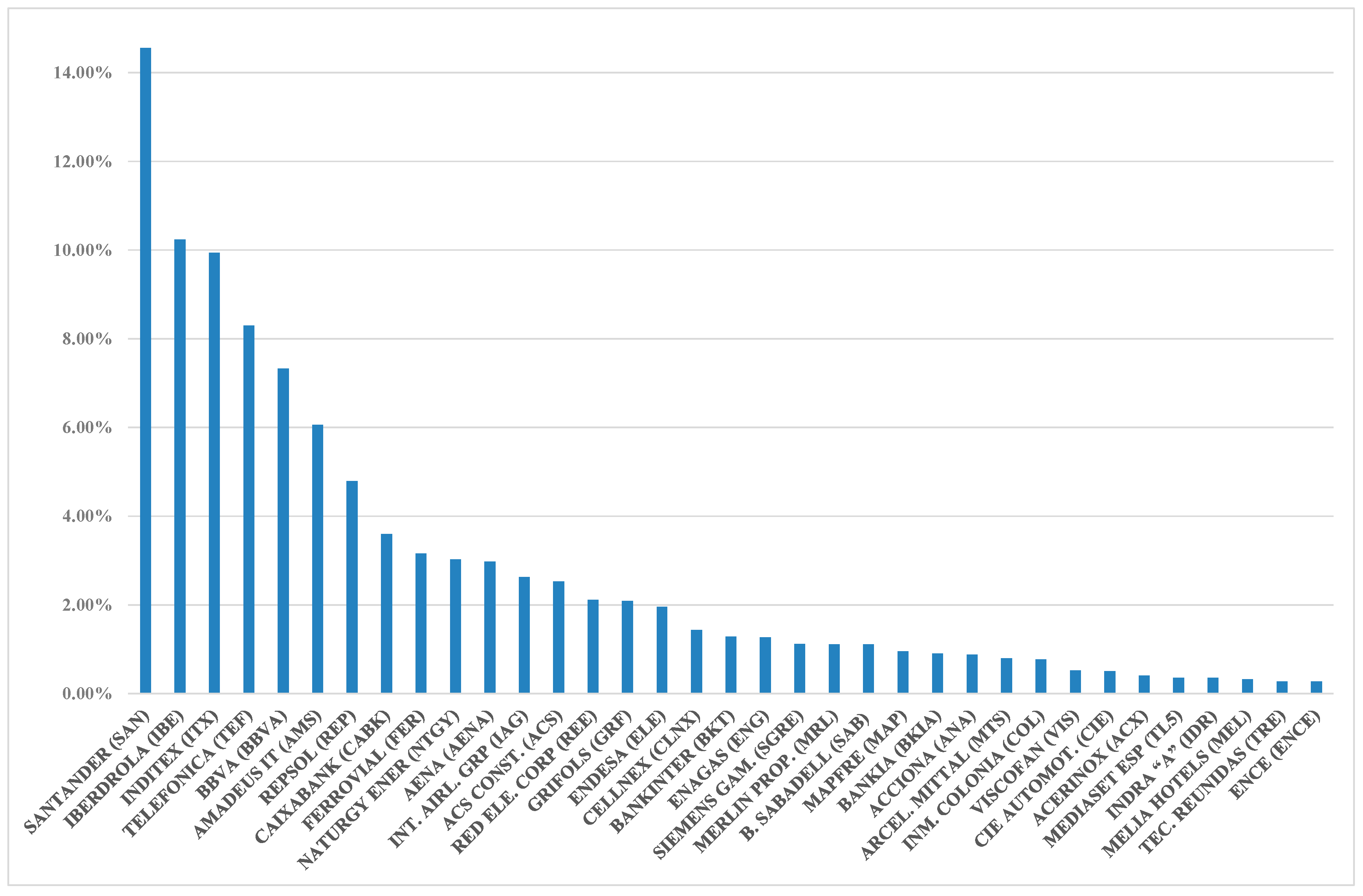
Thus, this paper analyses the consistency of the extensions of the Fama and French three- and five-factor models [1,2,3,4] in the Spanish stock market, approximated through the IBEX-35 market index. Specifically, the aim of this paper is to study the returns of the Spanish companies that currently comprise this index and their variation in response to changes in the risk factors proposed in the aforementioned extensions of the Fama and French models. With regard to the analysis period, this paper covers the period from January 2000 to December 2018. Moreover, for robustness, we split our sample period into three subperiods—precrisis, crisis and postcrisis—as the scenario changes according to the economic cycle. This analysis allows us to make a robust contrast of the results found in the estimates for the entire sample period, which could allow us to identify different sensitivities of stock returns depending on the stage of the economy.

On the other hand, this paper estimates the factor models proposed through the quantile regression (QR) technique, which provides numerous advantages over more traditional techniques. In addition, this paper focuses on the IBEX-35 companies’ returns of the Spanish stock market for several reasons. First, the Spanish market is one of the most relevant stock markets in the Eurozone [5]. Second, Spain has suffered the most from the consequences of the recent global financial crisis [6]. Third, in the context of the Fama and French factor models, not many studies analyse the Spanish market (with the exception of [4]) or include the Spanish market when the European markets are studied (see [7,8] and other studies at the company level in [9,10]).

Although some papers, such as [3,4], have carried out a study based on the Fama and French models, the present study contributes to the literature in the following three ways. First, we add three explanatory factors to the three- and five-factor Fama and French models [1,2]: momentum, reversal momentum and the liquidity factor. To the best of our knowledge, this study is the first to apply this extension to the Spanish stock market. Second, we compare the current five-factor model of Fama and French [2] with the original three-factor model of Fama and French [1] to determine which model best explains the Spanish companies’ returns for both the whole sample period and for the three subperiods to demonstrate the effect of the stage of the economic cycle in our results. Third, the method used to estimate the relationship between the variables is QR. This method provides information about the median and considers the different quantiles to observe how the variable behaves in the different theta values.

Specifically, this methodology addresses the relevant issue of asymmetries by analysing whether the sensitivity of the Spanish companies’ returns to changes in the explanatory factors changes across the quantiles, that is, in different states of the market. Moreover, this study analyses the potentially different behaviours and reactions of the Spanish companies in several (pre-, during and postcrisis) scenarios. Thus, our null hypothesis assumes that the sensitivity of the Spanish companies’ returns to changes in the risk factors included in the proposed factor models are quantile- and stage-of-the-economy-dependent. Specifically, we hypothesize that the greatest levels of explanatory power are at the extreme quantiles.

Finally, the rest of this research is divided into four sections. Section 2 includes a review of the literature. Section 3 presents the variables included in the study and the method used. Section 4 shows the most relevant results, including a robustness test. Finally, Section 5 presents the main conclusions of this study.

2. Literature Review

The financial literature has proposed different factor models to try to explain the behaviour of stock market returns. These models have been applied to different international markets and sample periods, the latter of which distinguish phases of expansion and recession.

The first generally accepted unifactorial model that appears in the financial literature is the capital asset pricing model (CAPM), which incorporates the stock market portfolio return as an explanatory factor. Since then, different multifactor models have emerged, adding other explanatory factors to the model.

One of the most well-known models is the Fama and French three-factor model [1], where the explanatory factors are the stock market return, size and growth. Subsequently, Fama and French expanded their previous model by adding profitability and investment risk factors, thus proposing the Fama and French five-factor model [2]. These two models have been applied in numerous studies, such as [11], who test both models on the CNX500 market in an emerging economy, India, and conclude that the five-factor model has greater explanatory power than the three-factor model does. [12] did the same in the Australian stock market, finding that the five-factor model provides an acceptable but still incomplete description of stock returns. The risk factors of profitability and investment have also been studied in papers such as [13], who studied stock returns in cases in which small companies invest greatly in return for low profitability, specifically in the USA. These companies are called “abnormal” because they invest a lot despite their low profitability, so the explanatory power of the profitability factor is limited for this type of company.

The five-factor model of Fama and French [2] observes some anomalies by examining the problems that occur when studying the low stock returns of companies that invest aggressively. Subsequently, [14] have analysed some international markets such as North America, Japan, Europe and Asia Pacific, focusing on the U.S. stock market. In North America, Europe and Asia Pacific, stock returns are positively related to the profitability factor and market portfolio returns, but decline with the investment factor. In Japan, stock returns are positively related to stock market returns, but have little to do with profitability and investment.

Later, [4] extend the Fama and French five-factor model by including additional explanatory factors such as the nominal and real interest rate and the expected inflation rate. Thus, [6] analyse the degree of exposure of Spanish sector stock returns to variations in interest rates by using the QR method and applying the Fama and French three-factor model (as in [15]). This research shows a statistically significant sensitivity that is more pronounced in times of crisis.

Finally, [3] conclude that other factors may also explain the sensitivity of stock market returns. This latest research proposes to include the risk factors momentum (MOM) and momentum reversal (LTREV) [16] and the liquidity factor negotiated (LIQV) [17] to extend the explanatory power of the Fama and French models.

The present research is focused on the extension of the Fama and French three- and five-factor models, according to [3], to study the behaviour of the Spanish companies’ returns to variations in the risk factors of these two models in the whole sample period and in three subperiods according to the economic cycle (called precrisis, crisis and postcrisis).

Additionally, regarding the reactions of companies to crisis, according to [9,10], the companies’ reaction (proactive/reactive) and the perception of uncertainty (high/low) would be connected, assuming that uncertainty essentially appears in times of economic turmoil. Thus, this perspective is very interesting when analysing the reaction of companies to crisis periods. [9], among others, suggest that companies characterized by a proactive behaviour show a riskier orientation, aimed at opportunity search and creation in times of economic downturns. However, companies with reactive behaviour present more passive and conservative profiles, reducing investments in innovative activities in crisis periods and focusing on short-term strategies.

In this way, a cyclical hypothesis suggests that investments in innovations increase in expansion periods, but decrease in economic turmoil. Therefore, some previous literature (such as [9,10]) assumes potential different responses and strategies towards crisis. Specifically, [10] suggest the pro-cyclicality and the counter-cyclicality hypothesis, and their results support the idea that proactiveness may be sensitive to the business cycle, because they assume that investments in innovation increase during economics expansions and decrease in recession periods. This point of view could be applied to our research to explain the potential different behaviour of Spanish companies’ stock returns to changes in some relevant risk factors included in our study.

To contribute to the previous literature, this study analyses the sensitivity of Spanish companies’ returns to changes in the explanatory factors across the quantiles, focusing on the relevant issue of potential asymmetries. Furthermore, this research examines whether the behaviour of Spanish companies in several (pre-, during and postcrisis) scenarios is different (or not). Specifically, we assume that the sensitivity of Spanish companies’ returns to changes in the risk factors included in the proposed factor models depends on the quantiles and the stage of the economy.

3. Data and Methodology

The third section of this paper is divided into two subsections. The first one, called data, details the main characteristics of the data used in this paper. The second subsection, called methodology, develops the methodology used in this research. Specifically, the first part of this subsection explains the QR methodology used in this paper. Meanwhile, the second part of the second subsection describes the two factor models studied in this paper, which are based on the Fama and French three- and five-factor models.

3.1. Data

This paper studies the sensitivity of the Spanish IBEX-35 companies’ returns between January 2000 and December 2018. In addition, for robustness, this full sample period is divided into three subperiods, thus analysing a precrisis subperiod (from January 2000 to January 2008), a crisis subperiod (from February 2008 to January 2014) and, finally, a postcrisis subperiod (from February 2014 to December 2018). The sample has been divided because, according to several authors, depending on the cycle of the economy, the sensitivity of company returns may vary based on changes in risk factors ([3,4,18], among others) (We selected the time references based on the Spanish National Statistics Institute and the Bank of Spain, which places the beginning of the Spanish crisis in 2008 and its recovery in 2014).

With regard to the periodicity of the data, monthly data collected from the investing website were used. In addition, the objective of this work is to analyse the companies that are currently included in the IBEX-35 market index. The components of the Spanish IBEX-35 index are shown in Figure 1, according to their percentage of participation in the index.

In the present study, two factor models are used that include a series of explanatory factors. On the one hand, we present the extended three-factor model of Fama and French [1], according to [3], composed of the following explanatory factors: stock market returns (R_M) proxied by IBEX-35 returns, the nominal interest rate (i), the size factor (SMB), the growth factor (HML), MOM, LTREV and LIQV. On the other hand, we present the extended five-factor model of Fama and French [2], which adds to the above explanatory factors the following factors: the profitability factor, RMW (Robust Minus Weak) and the investment factor, CMA (Conservative Minus Aggressive).

Data on the explanatory factors of the Fama and French models [1,2]—such as size, value or growth, profitability and investment and momentum and reversal momentum—have been collected from the Kennet French website (http://mba.tuck.dartmouth.edu/pages/faculty/ken.french/data_library.html). However, the traded liquidity factor data have been obtained from Pastor’s website (https://faculty.chicagobooth.edu/lubos.pastor/research).

The previous data chosen are the European risk factors because returns from the Spanish companies are estimated, and we have determined that these factors would be ideal for obtaining more conclusive results, according to [4,19], among others.

Next, we analyse the main descriptive statistics and the seasonality of all the variables in

Table 1. Descriptive statistics of companies’ and market returns and the rest of the explanatory factors.

	Mean	Median	Max.	Min.	Std. Dev.	Asymmetry	Kurtosis	Jarque-Bera	ADF	PP	KPSS
SAN	−0.0029	0.0073	0.3368	−0.2768	0.0872	−0.3309	4.3761	22.4401 ***	−14.3487 ***	−14.3383 ***	0.0276
IBE	0.0040	0.0074	0.1931	−0.2384	0.0649	−0.3228	4.5243	22.3852 ***	−14.3115 ***	−14.3118 ***	0.1269
ITX	0.0085	0.0086	0.1990	−0.2314	0.0652	−0.6686	4.8968	44.4357 ***	−13.2154 ***	−13.1967 ***	0.1049
TLF	−0.0059	−0.0038	0.2381	−0.2887	0.0721	−0.3345	4.2811	20.1040 ***	−16.8957 ***	−16.8957 ***	0.0976
BBVA	−0.0043	−0.0009	0.3040	−0.2821	0.0875	−0.01194	4.4542	18.2436 ***	−14.5442 ***	−14.5441 ***	0.0443
AMS	0.0160	0.0147	0.1250	−0.1474	0.0566	−0.56023	3.2120	5.79886 **	−12.0383 ***	−12.0720 ***	0.0641
REP	0.0006	0.0072	0.1732	−0.3433	0.0711	−1.0725	6.000	112.2299 ***	−12.8049 ***	−12.8049 ***	0.0666
CABK	−0.0033	0	0.2373	−0.2934	0.0931	−0.1482	3.8182	4.32276 *	−11.2153 ***	−11.2367 ***	0.0772
FER	0.0056	0.0079	0.3171	−0.3187	0.0792	−0.300	6.0634	80.3935 ***	−12.6804 ***	−12.8467 ***	0.0947
NTGY	0.0016	0.0055	0.1631	−0.2756	0.0678	−0.5076	4.292	22.5083 ***	−12.6054 ***	−12.7113 ***	0.0983
AENA	0.0109	0.0101	0.1283	−0.1083	0.0537	0.1916	2.3912	1.0566	−7.3471 ***	−7.31476 ***	0.1492
IAG	0.0085	0.0228	0.2022	−0.4624	0.0935	−1.7909	9.4368	221.5685 ***	−9.9676 ***	−10.013 ***	0.1221
ACS	0.0058	0.0139	0.2297	−0.3263	0.0753	−0.6443	5.5534	63.3956 ***	−13.5608 ***	−13.5608 ***	0.1538
REE	0.0102	0.0149	0.1396	−0.1234	0.0571	−0.2423	2.5804	3.3725	−14.5302 ***	−14.5883 ***	0.3751
GRF	0.0131	0.0135	0.2371	−0.2685	0.0842	−0.2103	3.1875	1.3606	−13.5848 ***	−13.5294 ***	0.1294
ELE	0.0025	0.0054	0.2174	−0.6365	0.0822	−2.3378	21.070	2758.109 ***	−14.8538 ***	−14.8254 ***	0.1240
CLNX	0.0135	0.0195	0.1985	−0.1237	0.0655	0.3726	3.1877	1.13176	−7.9627 ***	−7.9627 ***	0.1698
BKT	0.0023	0.0012	0.3344	−0.3088	0.0910	0.0102	4.3854	14.8771 ***	−10.9469 ***	−12.5371 ***	0.1168
ENG	0.0055	0.0069	0.2150	−0.1791	0.0582	−0.0471	3.7962	5.088 ***	−15.1887 ***	−15.1956 ***	0.1563
SGRE	0.0047	0.0197	0.3985	−0.6342	0.1192	−0.8461	6.9777	155.717 ***	−11.5790 ***	−12.1744 ***	0.1180
MRL	0.0070	0.0119	0.1220	−0.1016	0.0484	−0.1338	2.6442	0.4708	−6.9510 ***	−6.9296 ***	0.1108
SAB	0.0040	0.0057	0.1374	−0.2206	0.0523	−0.5533	4.4449	31.7431 ***	−13.8173 ***	−13.8334 ***	0.0904
MAP	0.0036	−0.0015	0.2740	−0.3323	0.0811	−0.3577	5.4651	54.6291 ***	−13.0419 ***	−13.0208 ***	0.1490
BKIA	−0.0213	−0.0126	0.689	−0.6779	0.1821	−0.1008	8.4696	112.3409 ***	−9.65057 ***	−9.6848 ***	0.0987
ANA	0.0034	0.0067	0.2267	−0.3664	0.0914	−0.6702	4.5620	32.8351 ***	−10.6089 ***	−11.7138 ***	0.1627
MTS	−0.0079	−0.0067	0.3719	−0.5600	0.1260	−0.6491	6.1944	74.8059 ***	−9.8659 ***	−9.8665 ***	0.0487
COL	−0.0191	−0.0033	0.3895	−0.5946	0.1445	−0.8613	6.2437	103.4151 ***	−10.2469 ***	−10.9179 ***	0.2115
VIS	0.0090	0.0149	0.2076	−0.1753	0.0566	−0.1165	4.2459	13.1874 ***	−15.1747 ***	−152872 ***	0.1126
CIE	0.0133	0.0074	0.3885	−0.3539	0.0914	−0.1628	6.7286	117.3224 ***	−14.4300 ***	−14.4800 ***	0.0886
ACX	−0.0004	0.0004	0.0302	−0.0532	0.0113	−1.2179	7.4188	197.3044 ***	−11.9968 ***	−12.0519 ***	0.3937
TL5	−0.0041	−0.0018	0.3173	−0.3012	0.0949	−0.1100	4.3697	14.1924 ***	−6.9540 ***	−12.7180 ***	0.0906
IDR	0.0022	0.0032	0.2296	−0.2322	0.0704	−0.1108	3.8179	5.9542 **	−14.0872 ***	−14.0852 ***	0.3156
MELL	0.0026	0.0069	0.5629	−0.5138	0.1089	−0.1358	8.6414	263.1685 ***	−13.5509 ***	−13.6310 ***	0.0801
TRE	0.0012	0.0092	0.1944	−0.4167	0.0884	−0.9057	5.8000	70.9006 ***	−8.4232 ***	−8.4212 ***	0.0997
ENC	0.0030	0.0159	0.2517	−0.3628	0.1026	−0.5536	3.7719	15.0312 ***	−12.1922 ***	−12.3068 ***	0.0938
RM (IBEX_35)	−0.0019	0.003	0.1537	−0.1882	0.0571	−0.3596	3.8029	11.1842 ***	−14.7357 ***	−14.7399 ***	0.0767
SMB	0.0011	0.0016	0.0486	−0.0693	0.0202	−0.4976	3.8788	16.9641 ***	−14.9194 ***	−14.9219 ***	0.0659
HML	0.0046	0.0038	0.1132	−0.0954	0.0260	0.5372	5.1836	56.7537 ***	−6.0685 ***	−12.6196 ***	0.9778
RMW	0.0030	0.0037	0.0638	−0.0488	0.0169	−0.2251	3.8279	8.5101 ***	−13.3470 ***	−13.3158 ***	0.1140
CMA	0.0035	0.0017	0.0875	−0.0725	0.0186	0.6950	6.6439	145.7634 ***	−12.0046 ***	−12.3646 ***	0.7803
MOM	0.0018	0.0037	0.1836	−0.3439	0.0534	−1.5054	12.6213	974.0149 ***	−15.0872 ***	−15.0921 ***	0.0591
LTREV	0.0029	0.0009	0.1621	−0.1461	0.0388	0.3938	7.0261	161.2873 ***	−16.7516 ***	−17.5382 ***	0.2151
LIQV	0.0046	0.0046	0.1119	−0.1278	0.0362	−0.2499	4.2180	16.3959 ***	−13.3194 ***	−13.2245 ***	0.6740
I	0.0376	0.0406	0.0676	0.0088	0.0147	−0.4528	2.1551	14.7636 ***	−1.0484	−1.0484	1.0198

Source: Own elaboration from the data obtained in Eviews. Note: This table presents the main statistics describing the monthly yields of the IBEX-35 companies and the explanatory variables of Models A and B for the full period from January 2000 to December 2018. These include: mean, median, minimum and maximum values, standard deviation, asymmetry and kurtosis. JB indicates the Jarque−Bera statistical test. The results of the ADF and Phillips−Perron (PP) unit root tests and the KPSS stationary test are included in the last three columns. As always, *, ** and *** indicate statistical significance at 10%, 5% and 1%, respectively.

. First, among the dependent variables, the company with the highest average return is Amadeus IT (AMS), followed by Cellnex (CLNX). In contrast, the company with the lowest average return is Bankia (BKIA), followed by Inmobiliaria Colonial (COL); both have negative returns.

The International Airlines Group (IAG) is the company with the highest median return, together with Siemens Gamesa (SGRE), Cellnex (CLNX) and Ence (ENC). However, BBVA shows the lowest median return in the sample period analysed.

To study the seasonality of the time series, three tests were carried out—two unit root tests (Augmented Dickey−Fuller (ADF) and Phillips−Perron (PP)) and a stationarity test (Kwiatkowski−Phillips−Schmidt−Shin (KPSS))—as shown in the last three columns of Table 1. According to the tests, all variables are stationary at a significance level of 1%.

Next, we analyse the main descriptive statistics for the explanatory factors (independent variables), which are collected in the last nine rows of Table 1. The variable with the highest average and median value is (i). Both the maximum value of the stock returns and the lowest minimum value correspond to the stock market index factor proxied by the IBEX-35 index.

Regarding the seasonality of the variables, we find that HML, CMA, LIQV and (i) are non-stationary variables. The transformation of the factors must be carried out by applying first differences. The decision has been made to carry out this process with (i) but not with the others (HML, CMA and LIQV) because they are original factors included in both of the models of Fama and French [1,2], and we prefer to maintain their conditions, as reflected in the models proposed by the authors.

3.2. Methodology

3.2.1. QR Methodology

As previously stated, the aim of this research is to analyse the IBEX-35 companies’ returns for changes in the explanatory variables included in the two factor models studied in this paper using the QR approach. This methodology was proposed by Koenker and Bassett in 1978 [20,21] and is considered an extension of the traditional method.

The main advantages of this methodology are the following. First, it provides a complete characterization of the conditional distribution of a dependent variable and not only its mean, as in the case of the ordinary least squares regression. Second, the QR methodology relaxes the restrictive assumption that error terms are identically distributed in all points of the conditional distribution, which implicitly recognizes heterogeneity. Furthermore, it offers more solid estimates in nonideal environments, as established by [6,19,22,23], among others.

Specifically, the QR approach provides a more complete picture of the linkages between stock returns and our explanatory variables because this model can be estimated for extreme tails of distributions of the dependent variables. Thus, this methodology addresses the relevant issue of asymmetries by analysing whether the sensitivity of Spanish companies’ returns to changes in the explanatory factors varies across the quantiles, that is, in different states of the markets. According to [24], this framework improves the strength of these relationships under different market scenarios. As parameters are quantile dependent, they can be different across the quantiles, showing potential symmetric and asymmetric patterns and indicating that these parameters can be affected by the innovation received at each period. Moreover, asymmetries are addressed in this research because this study analyses the potentially different behaviours and reactions of Spanish companies in pre-, during and postcrisis scenarios.

Recent papers ([25] among others) use the dynamic quantile autoregressive distributed lag (QARDL) model proposed by [26] that combines the autoregressive distributed lag model [27] and the QR approach [21]. The most relevant difference between QR and QARDL is that the last examines the long-run relationship with its related short-run movements over a range of quantiles ([24,26]. Although both methodologies are suitable to investigate the quantile-dependent relationships between related variables [28], the QARDL approach includes variables that have a mixed order of integration. As the unit root and stationary tests confirm the stationarity of our variables, then the QR (instead of QARDL) approach is a suitable choice for our research.

The QR model of Koenker and Basset [20,21] can be written as follows:

$$y_i= x_i{\beta }_{\theta }+u_{\theta i}·\mathrm{with}{Q}_{\theta } \left(y_i|x_i\right)= x_i{\beta }_{\theta }.$$

(1)

where y_i is the dependent variable; ${\beta }_{\theta }$ indicates an unknown k x 1 vector of regression parameters; and $Q_{\theta } \left(y_i|x_i\right)$, that is, the conditional quantile theta follows this assumption about the error term: $u_{\theta i}{Q}_{\theta } \left(u_{\theta }{x}_i\right)=0$. The QR estimates show a marginal change in the dependent variable at quantile theta to marginal changes in a particular regressor.

In addition, minimizing the following objective function with respect to β allows the vector of unknown parameter ${\beta }_{\theta }$:

$$[{{\displaystyle \sum }}_{i:y_i\ge x_{i{\beta }_i}}\theta \left|y_i-x_i\beta \right|+{{\displaystyle \sum }}_{y_{i<x_i{\beta }_i}}\left(1-\theta \right) \left|y_i- x_i\beta \right|]$$

(2)

In this minimization process, positive and negative residuals are differently weighted in each quantile [20]. Thus, theta values range between 0 and 1—specifically, 0.1, 0.25, 0.5, 0.75 and 0.9. Furthermore, ${\beta }_{ij}^{\theta }$ measures the sensitivity of stock return j at quantile theta to movements in factor i. The quantiles can be interpreted as follows: high values of theta are related to periods of expansion, and low values are associated with periods of recession ([23,29,30]; among others).

3.2.2. Extensions of the Fama and French Factor Models

In this section, we describe the two factor models proposed in the paper, which are extensions of the Fama and French three- and five-factor models [1,2].

Model A: Extension of the three-factor model of Fama and French [1]

This extension of the Fama and French three-factor model, proposed by [3], called Model A in this paper, is specified below:

$$R_{jt}- R_{Ft}= a_j+b_j·\left(R_{Mt}-R_{Ft}\right)+n_j· \Delta i_t^u+s_j·SM{B}_t+h_j· HM{L}_t+m_j· MO{M}_t+ v_j· LTRE{V}_t+ l_j·LIQ{V}_t+e_{jt}.$$

(3)

where R_jt is the IBEX-35 company returns, R_Ft is the risk-free return, R_Mt is the stock market return, $\Delta i_t^u$ is the unexpected change in the long-term nominal interest rate, SMB_t is the return on a diversified portfolio of small capitalization stocks minus the return on a diversified portfolio of large capitalization stocks (size factor), HML_t is the difference between the returns on diversified portfolios of high and low B/M stocks (value or growth factor), MOM_t is the average return on the two high prior return portfolios minus the average return on the two low prior return portfolios (MOM), LTREV_t is the average return on the two low prior return portfolios minus the average return on the two high prior return portfolios (LTREV), and LIQV_t is the weighted value on the weighted portfolio (10). Finally, e_jt is the error term.

Model B: Extension of the five-factor model of Fama and French [2]

The extension of the Fama and French five-factor model [2], proposed by [3], called Model B in this paper, is specified as below:

$$R_{jt}- R_{Ft}= a_j+b_j·\left(R_{Mt}-R_{Ft}\right)+n_j· \Delta i_t^u+s_j·SM{B}_t+h_j· HM{L}_t+r_j· RM{W}_t+c_j· CM{A}_t+m_j· MO{M}_t+ v_j· LTRE{V}_t+ l_j·LIQ{V}_t+e_{jt}$$

(4)

where RMW_t is the difference between the returns on diversified portfolios of stocks with robust and weak profitability (profitability factor), and CMA_t is the difference between the returns on diversified portfolios of the stocks of low- and high-investment firms (investment factor).

In both Models A and B, RM has been estimated with both the market return proposed by Fama and French and the return of the Spanish IBEX-35 stock market index.

4. Analysis of Results

This section shows the most relevant results extracted from the estimation of the two factor models proposed in this paper, called Models A and B, as extensions of the Fama and French three- and five-factor models, respectively. These two models study the sensitivity of the IBEX-35 companies’ returns to changes in all their explanatory factors. Additionally, these two factor models are estimated by QR following previous studies, such as [3,4,6,23], among others.

This section is divided into two subsections. The first subsection analyses the estimation results of both models in the whole sample period from January 2000 to December 2018. The second subsection contrasts the robustness of the results from the three subperiods according to different phases of the economic cycle—the precrisis subperiod (from January 2000 to January 2008), the during-crisis subperiod (from February 2008 to January 2014) and the postcrisis subperiod (from February 2014 to December 2018)—in line with [4].

4.1. Whole Sample Period

Table 2. Sensitivity of companies’ returns to variations in explanatory factors: Model A (extension of the Fama and French three-factor model) for the whole sample period.

	Theta = 0.1			Theta = 0.25			Theta = 0.5			Theta = 0.75			Theta = 0.9
	POS	NEG	TOTAL	POS	NEG	TOTAL	POS	NEG	TOTAL	POS	NEG	TOTAL	POS	NEG	TOTAL
RM	33	0	33	34	0	34	34	0	34	33	0	33	30	0	30
i	5	3	8	5	2	7	3	2	5	5	5	10	3	4	7
SMB	13	1	14	12	2	14	11	2	13	10	1	11	8	1	9
HML	2	5	7	6	4	10	7	8	15	7	9	16	3	6	9
MOM	2	2	4	3	1	4	1	1	2	1	3	4	4	4	8
LTREV	6	2	8	2	1	3	2	1	3	4	3	7	2	1	3
LIQV	4	3	7	3	2	5	1	1	2	3	3	6	4	4	8
TOTAL	65	16	81	65	12	77	59	15	74	63	24	87	54	20	74

Source: Own elaboration from Eviews data. Note: RM is the stock market return (minus the risk-free interest rate); i is the unexpected change in the long-term nominal interest rate; SMB is the return on a diversified portfolio of small capitalization stocks minus the return on a diversified portfolio of large capitalization stocks (size factor); HML is the difference between the returns on diversified portfolios of high and low B/M stocks (value or growth factor); MOM is the average return on the two high prior return portfolios minus the average return on the two low prior return portfolios (momentum factor); LTREV is the average return on the two low prior return portfolios minus the average return on the two high prior return portfolios (reversal momentum factor); and LIQV is the weighted value on the weighted portfolio (10).

and

Table 3. Sensitivity of companies’ returns to variations in explanatory factors: Model B (extension of the Fama and French five-factor model) for the whole sample period.

	Theta = 0.1			Theta = 0.25			Theta = 0.5			Theta = 0.75			Theta = 0.9
	POS	NEG	TOTAL	POS	NEG	TOTAL	POS	NEG	TOTAL	POS	NEG	TOTAL	POS	NEG	TOTAL
RM	33	0	33	34	0	34	34	0	34	34	0	34	31	0	31
i	4	1	5	3	2	5	2	3	5	4	5	9	3	5	8
SMB	10	2	12	8	4	12	7	2	9	8	0	8	10	1	11
HML	6	3	9	4	3	7	5	3	8	4	6	10	3	6	9
RMW	3	4	7	5	3	8	5	3	8	2	3	5	3	3	6
CMA	0	7	7	0	5	5	0	4	4	1	3	4	5	3	8
MOM	2	1	3	2	1	3	2	1	3	0	2	2	1	1	2
LTREV	5	1	6	4	0	4	1	1	2	2	2	4	1	4	5
LIQV	2	3	5	2	2	4	1	2	3	3	4	7	2	5	7
TOTAL	65	22	87	62	20	82	57	19	76	58	25	83	59	28	87

Source: Own elaboration from Eviews data. Note: RM is the stock market return (minus the risk-free interest rate); i is the unexpected change in the long-term nominal interest rate; SMB is the return on a diversified portfolio of small capitalization stocks minus the return on a diversified portfolio of large capitalization stocks (size factor); HML is the difference between the returns on diversified portfolios of high and low B/M stocks (value or growth factor); RMW is the difference between the returns on diversified portfolios of stocks with robust and weak profitability (profitability factor); CMA is the difference between the returns on diversified portfolios of the stocks of low- and high-investment firms (investment factor), MOM is the average return on the two high prior return portfolios minus the average return on the two low prior return portfolios (momentum factor); LTREV is the average return on the two low prior return portfolios minus the average return on the two high prior return portfolios (reversal momentum factor); and LIQV is the weighted value on the weighted portfolio (10).

collect the estimation results of the models proposed in this paper (Models A and B) for the whole sample period (from January 2000 to December 2018), distinguishing between positive and negative coefficients and indicating whether the variables are statistically significant.

As we can see, RM best explains the Spanish companies’ returns in 33 and 34 of 35 companies for Models A and B, respectively. Moreover, all these companies show positive and statistically significant sensitivity to variations in this factor, such as in [4].

With regard to (i), most companies show a positive sensitivity to changes in this variable in the lowest quantiles that becomes negative in the highest quantiles. SMB is the second most significant variable in both models (in terms of explanatory power). In this factor, a decreasing trend can be observed as the quantiles increase. However, in Model B, the explanatory variable presents more coefficients that are statistically significant in the extreme quantiles. These coefficients are positive in most companies. HML is the third most significant variable in both models. Moreover, Model A has more statistically significant variables than Model B does, especially in quantile 0.75. MOM is the least relevant factor in both models. The companies’ sensitivity to changes in LTREV is higher in the extreme quantiles, especially in Model B. Most companies have a positive sensitivity to this variable, which is more pronounced in the lowest quantiles. However, the 0.9 quantile of Model B has a clear negative sensitivity. This result also occurs in other previous studies, such as [3], where the U.S. market is analysed.

With regard to LIQV, Model A shows the same number of companies that have a positive and negative sensitivity. On the other hand, Model B shows more companies with a negative and statistically significant sensitivity.

Next, we analyse the explanatory factors that appear only in Model B: RMW and CMA. With respect to RMW, the lowest quantiles show a higher number of companies with statistically significant sensitivity to this factor without showing a clear sign about this sensitivity. However, according to CMA, the extreme quantiles (0.1 and 0.9) show the highest number of companies with statistically significant sensitivity to this factor. Specifically, the lowest quantiles exhibit an evident negative sensitivity that becomes positive in the highest quantile (0.9).

Furthermore, to analyse the explanatory power of our two factor Models A and B, the adjusted R² coefficient is studied in Figure 2. Specifically, this figure shows the mean (Panel A) and maximum (Panel B) values of the adjusted R² coefficient for Models A and B, distinguishing between different theta values (0.1, 0.25, 0.5, 0.75 and 0.9).

The mean adjusted R² coefficients of both Models A and B show a U-shape along the theta values, which means that these models will have a strong explanatory power in the extreme quantiles. In this case, the highest explanatory power corresponds to the lowest quantile 0.1. This result is in line with [3], where the best results of the adjusted R² are obtained at quantile 0.1.

On the other hand, considering the maximum adjusted R² values (Panel B) in Figure 2, we observe a U-shaped trend across the quantiles, showing a higher explanatory power of both models in the extremes and especially in the lowest quantile 0.1. Specifically, BBVA shows the maximum adjusted R² value in the full period for both models. Finally, this comparison between Models A and B in both panels of this figure confirms that Model B has higher values both in average and for the maximum adjusted R². Therefore, Model B is more effective in explaining the Spanish IBEX-35 companies’ returns to changes in explanatory risk factors.

4.2. Robustness Test

According to [3,4,18,23,30], among others, the sensitivity of stock market returns to changes in explanatory factors may vary depending on the stage of the economic cycle. Thus, a robustness test was performed on the two models presented in this paper to conduct a deep analysis of the results. This test distinguishes three subperiods of analysis: precrisis, during crisis and postcrisis.

4.2.1. Precrisis Subperiod (January 2000–January 2008)

This subsection analyses the IBEX-35 companies’ returns for the precrisis subperiod (between January 2000 and January 2008) for Models A and B, shown in

Table 4. Sensitivity of companies’ returns to variations in explanatory factors: Model A (extension of the Fama and French three-factor model) for the precrisis subperiod.

	Theta = 0.1			Theta = 0.25			Theta = 0.5			Theta = 0.75			Theta = 0.9
	POS	NEG	TOTAL	POS	NEG	TOTAL	POS	NEG	TOTAL	POS	NEG	TOTAL	POS	NEG	TOTAL
RM	20	0	20	22	0	22	20	0	20	18	0	18	17	0	17
i	4	4	8	3	3	6	2	2	4	2	1	3	1	3	4
SMB	8	2	10	4	2	6	3	1	4	5	1	6	4	1	5
HML	2	1	3	2	1	3	3	2	5	3	1	4	1	2	3
MOM	1	3	4	1	0	1	1	2	3	1	1	2	0	2	2
LTREV	2	0	2	1	0	1	2	1	3	2	1	3	1	1	2
LIQV	2	2	4	0	0	0	0	0	0	2	1	3	2	3	5
TOTAL	39	12	51	33	6	39	31	8	39	33	6	39	26	12	38

Source: Own elaboration from Eviews data. Note: RM is the stock market return (minus the risk-free interest rate); i is the unexpected change in the long-term nominal interest rate; SMB is the return on a diversified portfolio of small capitalization stocks minus the return on a diversified portfolio of large capitalization stocks (size factor); HML is the difference between the returns on diversified portfolios of high and low B/M stocks (value or growth factor); MOM is the average return on the two high prior return portfolios minus the average return on the two low prior return portfolios (momentum factor); LTREV is the average return on the two low prior return portfolios minus the average return on the two high prior return portfolios (reversal momentum factor); and LIQV is the weighted value on the weighted portfolio (10).

and

Table 5. Sensitivity of companies’ returns to variations in explanatory factors: Model B (extension of the Fama and French five-factor model) for the precrisis subperiod.

	Theta = 0.1			Theta = 0.25			Theta = 0.5			Theta = 0.75			Theta = 0.9
	POS	NEG	TOTAL	POS	NEG	TOTAL	POS	NEG	TOTAL	POS	NEG	TOTAL	POS	NEG	TOTAL
RM	22	0	22	22	0	22	19	0	19	20	0	20	19	0	19
i	5	3	8	2	4	6	1	2	3	3	1	4	3	3	6
SMB	5	3	8	2	2	4	3	1	4	5	1	6	4	2	6
HML	2	0	2	2	0	2	2	1	3	2	1	3	3	1	4
RMW	1	1	2	3	1	4	2	1	3	3	3	6	2	5	7
CMA	1	1	2	0	0	0	0	1	1	1	1	2	2	1	3
MOM	1	2	3	2	1	3	0	1	1	1	4	5	1	2	3
LTREV	2	1	3	1	0	1	1	0	1	2	0	2	2	0	2
LIQV	0	2	2	1	1	2	1	1	2	3	2	5	3	3	6
TOTAL	39	13	52	35	9	44	29	8	37	40	13	53	39	17	56

Source: Own elaboration from Eviews data. Note: RM is the stock market return (minus the risk-free interest rate); i is the unexpected change in the long-term nominal interest rate; SMB is the return on a diversified portfolio of small capitalization stocks minus the return on a diversified portfolio of large capitalization stocks (size factor); HML is the difference between the returns on diversified portfolios of high and low B/M stocks (value or growth factor); RMW is the difference between the returns on diversified portfolios of stocks with robust and weak profitability (profitability factor); CMA is the difference between the returns on diversified portfolios of the stocks of low- and high-investment firms (investment factor), MOM is the average return on the two high prior return portfolios minus the average return on the two low prior return portfolios (momentum factor); LTREV is the average return on the two low prior return portfolios minus the average return on the two high prior return portfolios (reversal momentum factor); and LIQV is the weighted value on the weighted portfolio (10).

, respectively.

As in the full sample, RM best explains the behaviour of the IBEX-35 companies’ returns in approximately an average of 19 and 20 of 25 companies for Models A and B, respectively. In all cases, this sensitivity is positive and statistically significant. We can also observe that more firms have statistically significant results in the lowest quantile, coinciding with [4].

With regard to (i), the companies present both positive and negative sensitivity, as in the whole sample period. If we analyse the quantiles, in Model A, the trend across the quantiles is decreasing, with the highest values in the lowest quantiles. However, in Model B, the trend is U-shaped, i.e., the extreme quantiles have more statistically significant firms.

For SMB, the 0.1 quantile stands out, where more companies have statistically significant coefficients (the majority positive) coinciding with the whole sample period. Regarding HML, we observe that, in Model A, more companies show statistically significant coefficients than they do in Model B.

When analysed, MOM ceases to be the least relevant factor, as it was in the entire sample. The sensitivity shown through the value and sign of the coefficients becomes mostly negative, coinciding with [3]. For the explanatory variable LTREV, most companies have a positive sensitivity to this variable in a stable way along the quantiles.

Next, we analyse LIQV in Model A, and we observe that the extreme quantiles show better results. However, in Model B, the best results are in the highest quantiles (0.75 and 0.9), where more companies have a notable liquidity factor.

Regarding RMW and CMA, the sensitivity to changes in the RMW variable has an increasing tendency, in contrast to the decreasing tendency of the full sample period. However, the results obtained for the CMA factor coincide with the whole sample period because their values are higher in the extreme quantiles.

Figure 3 collects the data of the mean and maximum adjusted R² coefficients in the precrisis subperiod. In this subperiod, Model B explains, better than Model A does, the Spanish companies’ returns throughout the selected explanatory factors. We emphasize that the average and the maximum adjusted R² coefficients are higher in the extreme quantiles, and are the highest at quantile 0.1, according to the full sample period. Thus, both panels show a U-shaped evolution along with theta values. Additionally, the maximum explanatory power corresponds to BBVA, coinciding with the full period.

This precrisis subperiod is better explained than the entire sample period because the average and maximum adjusted R² of both models are, respectively, over 33% (vs. 29% in the full period) and over 67% (vs. 64% in the full period).

4.2.2. Crisis Subperiod (February 2008–January 2014)

In this subsection, we analyse the IBEX-35 companies’ returns for the second part of the period, called the crisis subperiod, which runs from February 2008 to January 2014 for Models A and B in

Table 6. Sensitivity of companies’ returns to variations in explanatory factors: Model A (extension of the Fama and French three-factor model) for the crisis subperiod.

	Theta = 0.1			Theta = 0.25			Theta = 0.5			Theta = 0.75			Theta = 0.9
	POS	NEG	TOTAL	POS	NEG	TOTAL	POS	NEG	TOTAL	POS	NEG	TOTAL	POS	NEG	TOTAL
RM	16	0	16	19	0	19	22	0	22	19	0	19	18	0	18
i	4	3	7	3	0	3	3	1	4	3	1	4	4	1	5
SMB	4	0	4	5	1	6	4	0	4	3	1	4	3	1	4
HML	4	2	6	1	2	3	0	2	2	3	1	4	2	0	2
MOM	2	3	5	1	1	2	2	2	4	2	4	6	2	2	4
LTREV	2	0	2	4	2	6	0	0	0	1	0	1	0	4	4
LIQV	5	1	6	2	1	3	4	1	5	1	2	3	1	2	3
TOTAL	37	9	46	35	7	42	35	6	41	32	9	41	30	10	40

Source: Own elaboration from Eviews data. Note: RM is the stock market return (minus the risk-free interest rate); i is the unexpected change in the long-term nominal interest rate; SMB is the return on a diversified portfolio of small capitalization stocks minus the return on a diversified portfolio of large capitalization stocks (size factor); HML is the difference between the returns on diversified portfolios of high and low B/M stocks (value or growth factor); MOM is the average return on the two high prior return portfolios minus the average return on the two low prior return portfolios (momentum factor); LTREV is the average return on the two low prior return portfolios minus the average return on the two high prior return portfolios (reversal momentum factor); and LIQV is the weighted value on the weighted portfolio (10).

and

Table 7. Sensitivity of companies’ returns to variations in explanatory factors: Model B (extension of the Fama and French five-factor model) for the crisis subperiod.

	Theta = 0.1			Theta = 0.25			Theta = 0.5			Theta = 0.75			Theta = 0.9
	POS	NEG	TOTAL	POS	NEG	TOTAL	POS	NEG	TOTAL	POS	NEG	TOTAL	POS	NEG	TOTAL
RM	18	0	18	21	0	21	22	0	22	21	0	21	21	0	21
i	4	3	7	3	0	3	2	1	3	2	3	5	4	1	5
SMB	5	0	5	6	0	6	8	0	8	3	2	5	2	1	3
HML	1	1	2	1	1	2	1	1	2	3	1	4	5	1	6
RMW	0	0	0	2	1	3	0	1	1	0	0	0	3	0	3
CMA	1	4	5	0	3	3	0	2	2	1	2	3	3	3	6
MOM	1	1	2	2	1	3	3	1	4	2	1	3	2	2	4
LTREV	2	0	2	2	2	4	0	0	0	2	1	3	0	2	2
LIQV	1	0	1	1	0	1	0	1	1	1	2	3	1	2	3
TOTAL	33	9	42	38	8	46	36	7	43	35	12	47	41	12	53

Source: Own elaboration from Eviews data. Note: RM is the stock market return (minus the risk-free interest rate); i is the unexpected change in the long-term nominal interest rate; SMB is the return on a diversified portfolio of small capitalization stocks minus the return on a diversified portfolio of large capitalization stocks (size factor); HML is the difference between the returns on diversified portfolios of high and low B/M stocks (value or growth factor); RMW is the difference between the returns on diversified portfolios of stocks with robust and weak profitability (profitability factor); CMA is the difference between the returns on diversified portfolios of the stocks of low- and high-investment firms (investment factor), MOM is the average return on the two high prior return portfolios minus the average return on the two low prior return portfolios (momentum factor); LTREV is the average return on the two low prior return portfolios minus the average return on the two high prior return portfolios (reversal momentum factor); and LIQV is the weighted value on the weighted portfolio (10).

, respectively.

RM remains the factor that best explains the companies’ returns, although in this subperiod, the number of companies with statistically significant coefficients decreases considerably. In concrete terms, on average, 19 and 21 of 29 companies are sensitive to this factor in Models A and B, respectively. In this subperiod, Model B (vs. A) shows the highest number of companies with statistically significant sensitivity. Moreover, the quantiles with the best results are in the middle of the distribution.

(i) is the second explanatory variable with positive sensitivity. In addition, the extreme quantiles have more companies that are statistically significant.

SMB clearly has a positive sensitivity. In Model B, the largest number of statistically significant coefficients is located in the 0.5 quantile. With respect to HML, Model A has more companies with a positive and statistically significant sensitivity. Moreover, this sensitivity is higher than that in the previous subperiod.

MOM shows a negative sensitivity in Model A. On the other hand, the coefficients are positive in Model B, coinciding with [3]. LTREV exhibits a positive sensitivity in the lower quantiles, but in the higher quantiles, it becomes negative, as in the full sample period.

On the other hand, the trend in LIQV in this subperiod begins positive in the low quantiles and becomes negative in the high quantiles. Both Models A and B exhibit the same trend, but more companies are statistically significant in Model A.

Finally, coefficients associated with RMW are very low, being positive in most cases as in the total sample and the precrisis subperiod, coinciding with the results of [3]. With regard to CMA, its values are higher in the extreme quantiles.

Additionally, Figure 4 plots the mean and maximum adjusted R² coefficients across quantiles, presenting a U-shaped evolution. Thus, the explanatory power of both models in both panels is higher in the extreme quantiles, especially at quantile 0.1, and, in general, Model B explains the Spanish companies’ returns (except for theta 0.5) better than Model A does. Moreover, BBVA has the maximum adjusted R² value, according to the full period and the precrisis subperiod. On the other hand, this crisis subperiod is better explained with both models than the whole sample period is. For example, the average and the maximum adjusted R²s of Model B in this subperiod are, respectively, close to 34% and 68%, while in the full period, they are close to 29% and 64%, respectively, at quantile 0.1.

4.2.3. Postcrisis Subperiod (February 2014–December 2018)

Table 8. Sensitivity of companies’ returns to variations in explanatory factors: Model A (extension of the Fama and French three-factor model) for the postcrisis subperiod.

	Theta = 0.1			Theta = 0.25			Theta = 0.5			Theta = 0.75			Theta = 0.9
	POS	NEG	TOTAL	POS	NEG	TOTAL	POS	NEG	TOTAL	POS	NEG	TOTAL	POS	NEG	TOTAL
RM	29	0	29	29	0	29	29	0	29	27	0	27	24	0	24
i	5	4	9	4	2	6	3	1	4	2	3	5	6	2	8
SMB	5	3	8	4	3	7	3	4	7	3	2	5	3	3	6
HML	4	7	11	3	5	8	5	7	12	5	11	16	4	8	12
MOM	6	2	8	6	1	7	6	1	7	3	2	5	3	5	8
LTREV	4	2	6	0	0	0	0	1	1	1	1	2	0	3	3
LIQV	0	2	2	0	0	0	1	0	1	2	1	3	2	2	4
TOTAL	53	20	73	46	11	57	47	14	61	43	20	63	42	23	65

Source: Own elaboration from Eviews data. Note: RM is the stock market return (minus the risk-free interest rate); i is the unexpected change in the long-term nominal interest rate; SMB is the return on a diversified portfolio of small capitalization stocks minus the return on a diversified portfolio of large capitalization stocks (size factor); HML is the difference between the returns on diversified portfolios of high and low B/M stocks (value or growth factor); MOM is the average return on the two high prior return portfolios minus the average return on the two low prior return portfolios (momentum factor); LTREV is the average return on the two low prior return portfolios minus the average return on the two high prior return portfolios (reversal momentum factor); and LIQV is the weighted value on the weighted portfolio (10).

and

Table 9. Sensitivity of companies’ returns to variations in explanatory factors: Model B (extension of the Fama and French five-factor model) for the postcrisis subperiod.

	Theta = 0.1			Theta = 0.25			Theta = 0.5			Theta = 0.75			Theta = 0.9
	POS	NEG	TOTAL	POS	NEG	TOTAL	POS	NEG	TOTAL	POS	NEG	TOTAL	POS	NEG	TOTAL
RM	31	0	31	31	0	31	31	0	31	29	0	29	27	0	27
i	0	4	4	1	2	3	0	1	1	0	2	2	1	2	3
SMB	6	3	9	4	1	5	5	2	7	4	2	6	7	3	10
HML	5	3	8	2	1	3	3	2	5	1	6	7	2	5	7
RMW	6	3	9	4	3	7	3	3	6	3	3	6	2	5	7
CMA	1	3	4	0	3	3	0	3	3	1	1	2	2	0	2
MOM	5	3	8	3	0	3	2	1	3	1	3	4	4	3	7
LTREV	1	1	2	1	0	1	0	0	0	1	2	3	0	3	3
LIQV	1	1	2	0	0	0	0	0	0	2	0	2	2	1	3
TOTAL	56	21	77	46	10	56	44	12	56	42	19	61	47	22	69

Source: Own elaboration from Eviews data. Note: RM is the stock market return (minus the risk-free interest rate); i is the unexpected change in the long-term nominal interest rate; SMB is the return on a diversified portfolio of small capitalization stocks minus the return on a diversified portfolio of large capitalization stocks (size factor); HML is the difference between the returns on diversified portfolios of high and low B/M stocks (value or growth factor); RMW is the difference between the returns on diversified portfolios of stocks with robust and weak profitability (profitability factor); CMA is the difference between the returns on diversified portfolios of the stocks of low- and high-investment firms (investment factor), MOM is the average return on the two high prior return portfolios minus the average return on the two low prior return portfolios (momentum factor); LTREV is the average return on the two low prior return portfolios minus the average return on the two high prior return portfolios (reversal momentum factor); and LIQV is the weighted value on the weighted portfolio (10).

show the results for the estimates of the IBEX-35 Spanish companies’ returns to changes in the explanatory factors included in Models A and B for the postcrisis subperiod (from February 2014 to December 2018).

RM best explains the Spanish companies’ returns in this postcrisis subperiod (and in the full period and the two previous subperiods), with a positive and statistically significant sensitivity for an average of 28 and 30 of the 35 companies in Models A and B, respectively. Additionally, Model B (vs. Model A) and the lowest quantiles (vs. highest quantiles) show the highest number of companies with a positive sensitivity and statistical significance.

As for (i), the two models exhibit differences. In the first model, the sensitivity is, in most cases, positive. However, in the second model, the negative sign of the explanatory factor prevails, such as in [4]. In both models, the extreme quantiles are those with the highest statistically significant coefficients.

SMB clearly has a positive coefficient, especially in Model B. Moreover, in Model B, the greatest numbers of statistically significant coefficients are located in the extreme quantiles, in line with other works such as [3]. With respect to HML, both models show a negative sensitivity to changes in this factor, as shown in [3], which indicates that, in times of expansion, the sign is negative.

MOM and LTREV show that, in times of expansion, the sensitivity of the companies’ returns to changes in these risk factors is positive, especially in the low quantiles. As previously advanced, at the higher quantiles, the sign becomes negative.

On the other hand, LIQV shows very few statistically significant companies, especially in Model B (i.e., in the quantiles 0.25 and 0.5, no company has statistical significance). In the highest quantiles, some companies have negative sensitivity to this risk factor.

With regard to the specific factors of Model B RMW and CMA, in this postcrisis subperiod, during a clear expansion stage of the economy, the trend in RMW is linear in terms of statistically significant coefficients, although the sign varies: in the lowest quantiles, the sign is positive, but it becomes negative at the highest quantiles. With respect to CMA, the lowest quantiles have more statistically significant coefficients, and their sign is negative, although they become positive in the highest quantiles.

Figure 5 shows the results of the adjusted R² coefficients for the postcrisis subperiod. The best results are in the extreme quantiles, specifically, in quantile 0.1. In this subperiod, Model B explains the IBEX-35 companies’ returns better than Model A does in all of the quantiles, with the largest difference between models in all periods. For example, in the extreme quantile 0.1, Model B reaches a mean adjusted R² of 34% (vs. 31% in Model A) and a maximum adjusted R² of 64% (vs. 61% for Model A). Additionally, this postcrisis subperiod is better explained with both models than the entire sample period, especially in the highest quantiles. As an example, the maximum adjusted R² of Model B at quantile 0.9 in this subperiod is close to 63%, while in the full period, it is close to 59%. The maximum adjusted R² values in this postcrisis subsample at quantile 0.1 are slightly superior to those in the full sample (63.99% vs. 63.86%, respectively). Additionally, in this subperiod, the maximum explanatory power corresponds to Santander, in contrast to previous periods, where the maximum adjusted R² corresponded to BBVA. However, this result is in line with those obtained in the rest of the periods because both companies belong to the same banking sector.

Finally, both panels in this figure corroborate the trend observed in all the periods (the full period and the three subperiods) analysed in this paper. This trend consists of a U-shaped evolution of mean and maximum adjusted R² coefficients as the values of theta increase. Therefore, these models may have a greater explanatory power in the extreme quantiles in all periods, confirming the suitability of using this methodology of regression by quantiles in this kind of research. Moreover, this research concludes that the best result of the adjusted R² corresponds to the lowest quantile, 0.1. Thus, this result, which is consistent in all subperiods, coincides with [3,4,18,29], among others.

Regarding the economic meaning of the results, according to [6,31,32,33,34], the Fama and French factors are capable of predicting some macroeconomic variables, especially economic growth and default risk. In this sense, our findings suggest that Spanish companies would respond to this capability of Fama and French factors (mainly, size, value, momentum and investment), because we find more statistically significant sensitivities in the high and low states of the market. In addition, our results would evidence the poor performance of Spanish companies during the global financial crisis, mainly due to the deteriorating economic outlook in Spain.

5. Conclusions

This paper analyses the sensitivity of the Spanish stock market at the company level to changes in different risk factors commonly accepted in the financial literature. For this purpose, we compare two factor models (called Models A and B in this paper) based on the extended three- and five- models of Fama and French [1,2] to explain the behaviour of the IBEX-35 companies’ returns in the period between January 2000 and December 2018. The QR method is used to obtain the best possible estimate. Moreover, we divide the entire sample period (January 2000–December 2018) into three subperiods: precrisis (January 2000–January 2008), crisis (February 2008–January 2014) and postcrisis (February 2014–December 2018). This division allows us to contrast the robustness of the results and the different behaviours of our two models depending on the stage of the economic cycle.

Regarding this paper’s conclusions about the explanatory factors of the two models analysed in it, several variables have similar behaviours in all periods. These variables include RM, which shows the most statistically significant coefficients, and which shows a positive sign for most companies, especially in the full period and in the postcrisis subperiod. Specifically, on average, between the quantiles, approximately 94% and 97% for Models A and B, respectively, of the companies show positive sensitivity to variations in this factor in the full period. Consistently, for Models A and B respectively, 76% and 80% in the precrisis subperiod, 65% and 72% in the crisis subperiod and 80% and 86% of the companies show the same behaviour. Moreover, Model B shows a higher number of the companies with positive and statistically significant sensitivity to variations in this factor in all periods. In addition, the lowest quantiles have more statistically significant companies in most periods.

On the other hand, the nominal interest rate (i) varies during the analysis, depending on the stage of the economic cycle. In all periods, Model A (vs. B) has more statistically significant coefficients. With respect to the sign, in the lowest quantiles, it is positive, and as we advance in theta values, this sign becomes negative in most periods. The crisis subperiod has more statistically significant coefficients to changes in this risk factor than, in general, to variations in the rest of explanatory factors. This result is relevant, as it could suggest that the variable interest rate has a greater impact on Spanish companies’ returns in the stages of economic recession. In addition, the observed sign would determine that changes in interest rates imply changes in business returns in different directions at low theta values, while they imply changes in the same direction at high theta values.

We observe the same trend with MOM and LTREV in most periods. The sensitivity of the companies’ returns to variations in these two risk factors is positive in the low quantiles and becomes negative as we move towards the high quantiles. Moreover, for the first variable, MOM, a higher number of companies show statistically significant coefficients than for the second variable, LTREV, in most periods, especially in the last subperiod. Additionally, in both factors, most statistically significant coefficients are in the extreme quantiles. These results confirm that the methodology used in this paper is appropriate.

SMB is one of the most significant variables explaining the behaviour of companies’ returns. Specifically, it presents a positive and statistically significant sensitivity in all periods and models, mainly in the crisis subperiod according to [3]. With regard to HML, results were inconsistent, but the variable is the second most significant (after RM) for the first model in the postcrisis subperiod and for the full period. Meanwhile, the least relevant factor in terms of statistical significance is LIQV, as even at the medium quantiles (especially in the precrisis and postcrisis subperiods) no companies have statistically significant coefficients.

Regarding the specific factors of Model B, the trend in RMW is linear in terms of statistically significant coefficients. Moreover, the sign of these coefficients is positive in the lowest quantiles and becomes negative in the highest quantiles in most periods (except for the crisis subperiod, where this factor is not relevant). With respect to CMA, the extreme quantiles in most periods have many statistically significant coefficients (except for the postcrisis subperiod, where the trend is decreasing). These coefficients are positive in the low quantiles, but become negative as we advance towards the high quantiles in all periods.

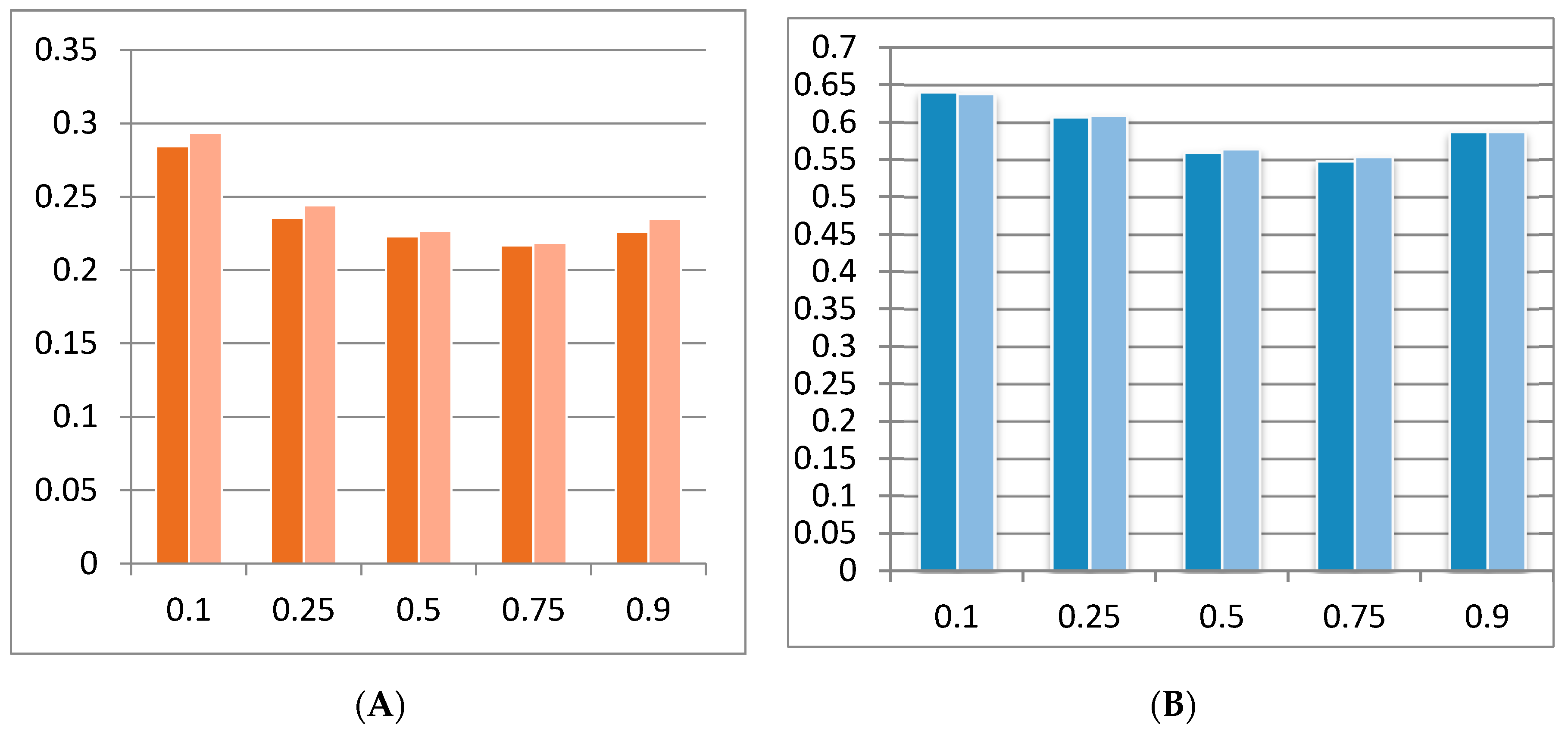
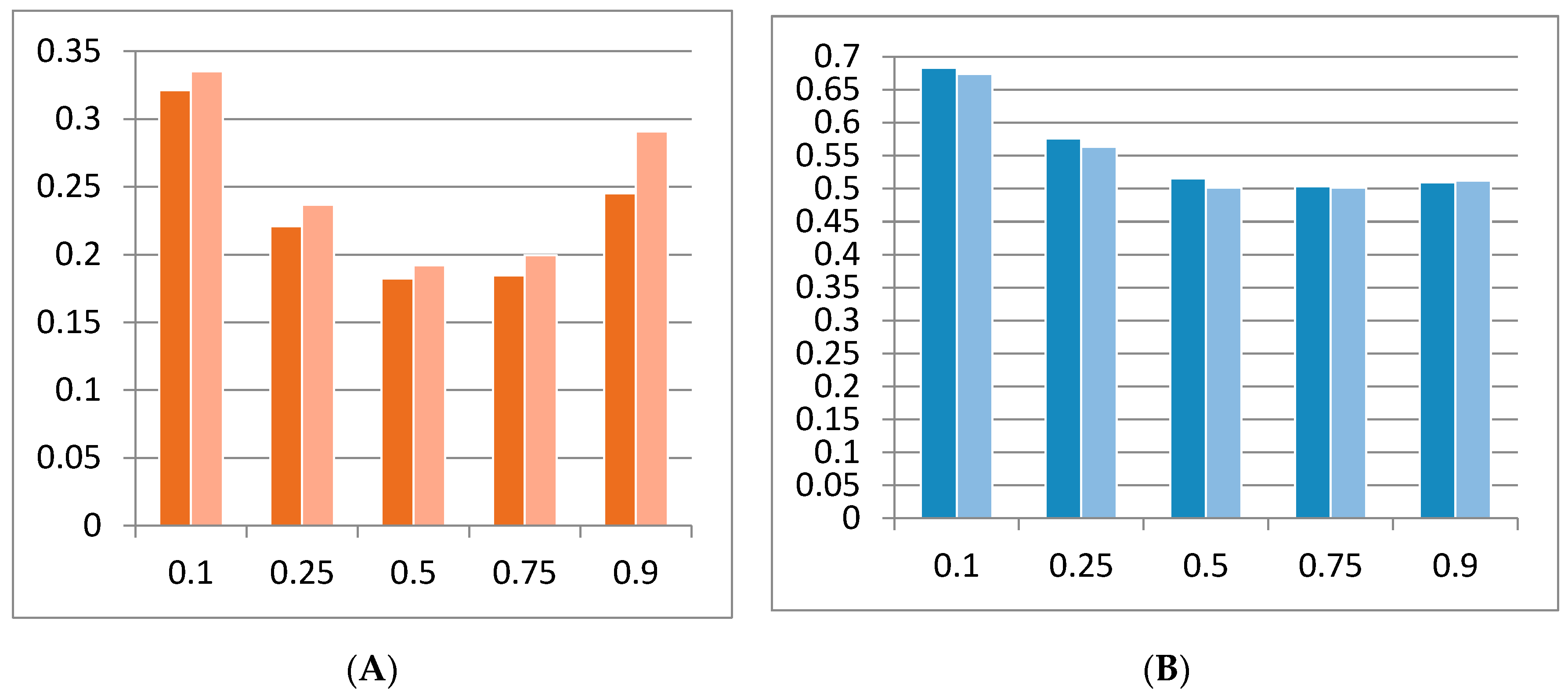
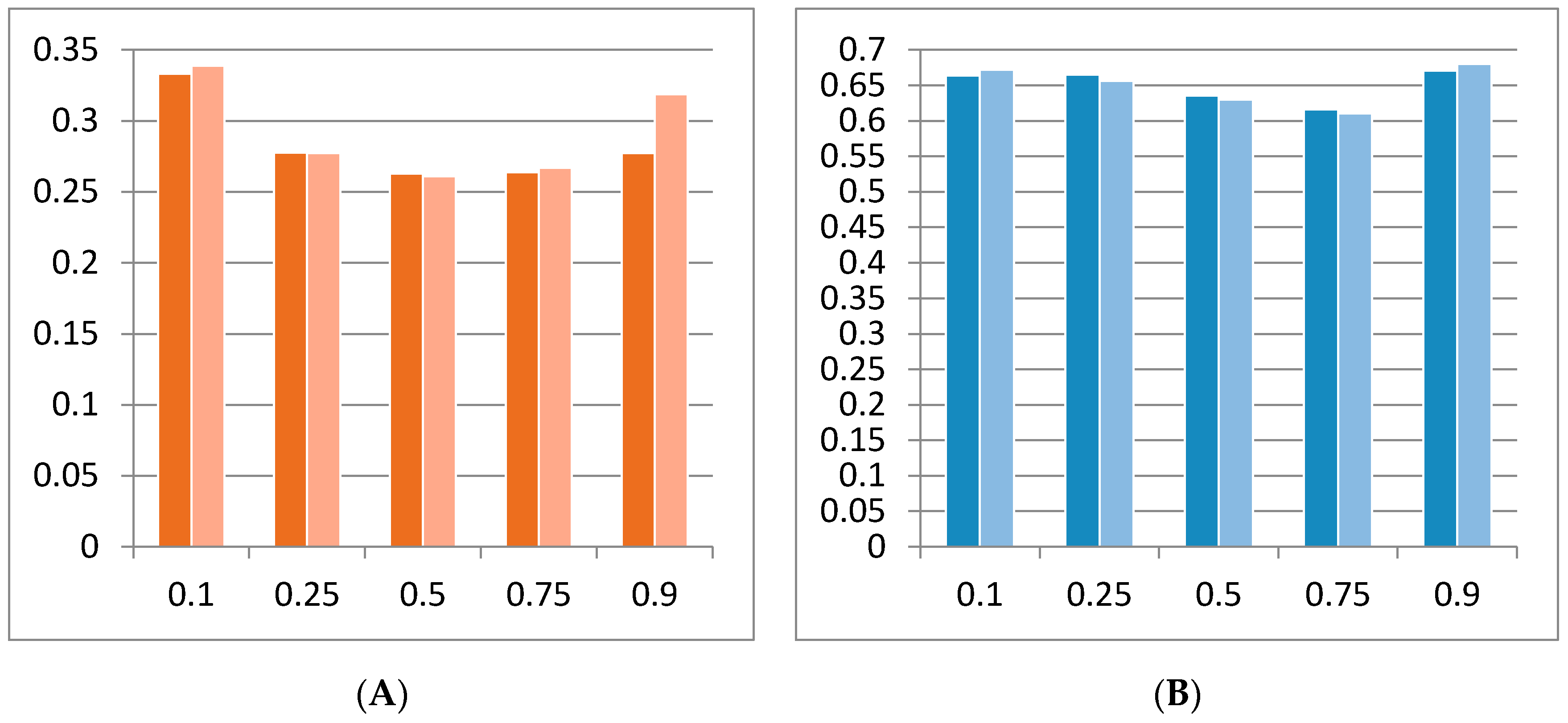
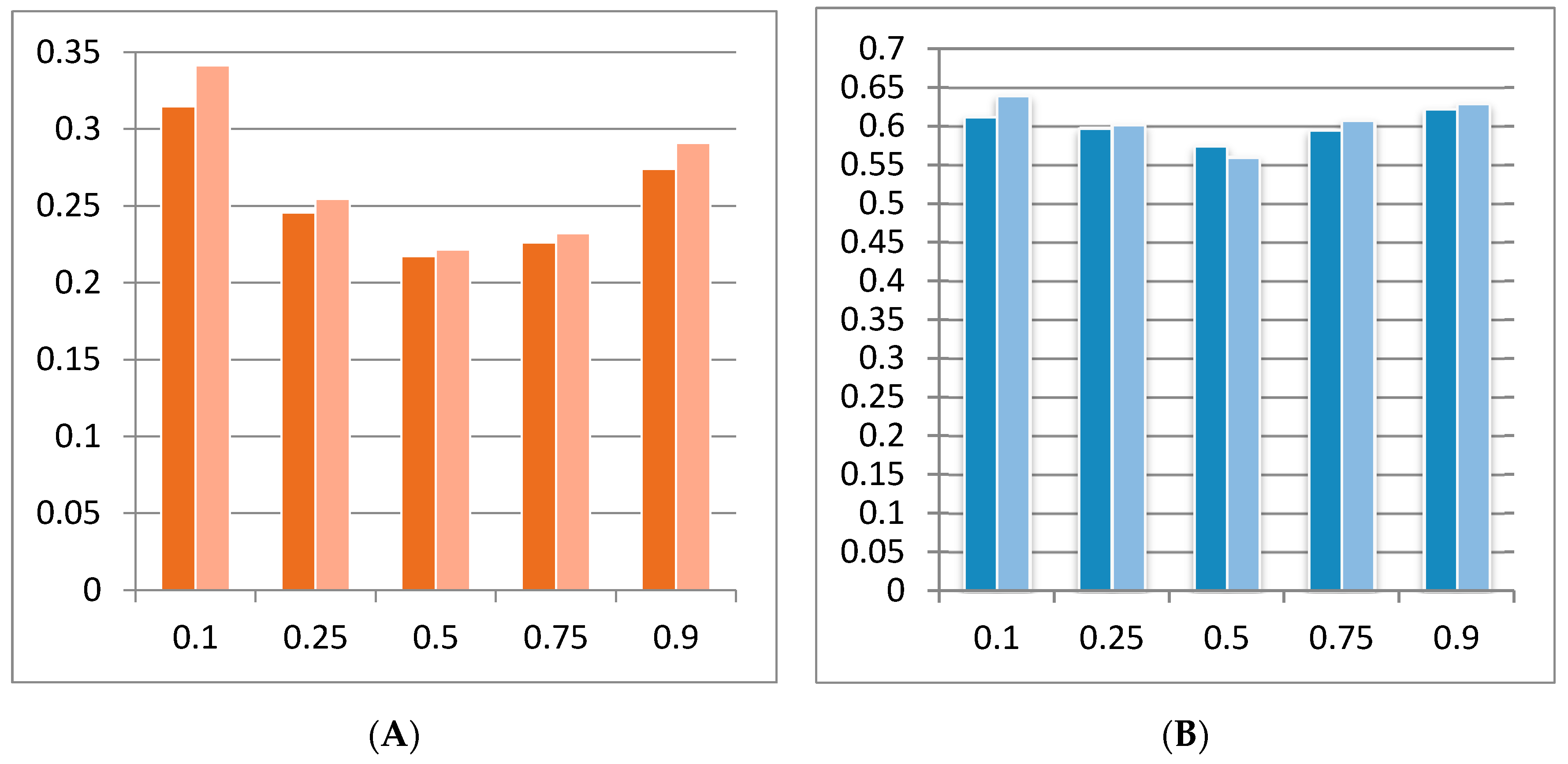
Finally, focusing on the explanatory power, we obtain several conclusions. First, the trend observed in all periods and subperiods has been corroborated, which consists of an evolution of the explanatory power in the U-shape as the value of theta increases in both models and in both mean and maximum adjusted R². Thus, these models have the greatest explanatory power in the extreme quantile and, specifically, in the lowest quantile, 0.1, in line with previous studies such as [3]. Second, Model B explains the Spanish companies’ returns better than Model A does in the full period and in the three subsample periods. Third, BBVA has the maximum adjusted R² value in all periods, except for the postcrisis subperiod, where the maximum explanatory power corresponds to Santander. Thus, Models A and B best explain stock returns for companies that belong to the same banking sector. Fourth, the crisis subperiod is the economic stage with the highest values of this coefficient (adjusted R²) in all of the quantiles. Therefore, the proposed factor models and, in particular, the second model, explain the variations in Spanish companies’ returns the best in crisis stages.

For all these reasons, we can justify the relevance of the QR approach when estimating the models proposed in the whole sample period and in the contrast of robustness proposed in this research. Both analyses have allowed us to study in depth the sensitivity of the Spanish companies’ returns to changes in the risk factors included in the proposed factor Models A and B based on the well-known Fama and French three- and five-factor models.

This methodology has allowed the detection of asymmetries in the behaviours and reactions of Spanish companies’ returns to changes in some explanatory factors across the quantiles in several (pre-, during and postcrisis) subperiods. Our null hypothesis has been accepted, confirming that the sensitivity of the Spanish companies’ returns to changes in the risk factors included in the proposed factor models are quantile- and stage-of-the-economy-dependent, reaching the greatest levels of explanatory power at the extreme quantiles.

Policy recommendations would consist of following the strategies implemented in companies that have reduced the negative consequences in times of financial crisis. Furthermore, a crucial implication for market participants would be that investors should consider the regime-dependent nature of the companies’ sensitivity to changes in the risk factors. Therefore, this suggestion would have implications for risk management and economic policy decisions, mainly during crisis periods.

Our research raises questions for further research regarding the sensitivity of Spanish companies’ stock returns to changes in relevant risk factors across the quantiles and in pre-, during and postcrisis scenarios. Our results confirm the different behaviours and reactions of Spanish companies in different stages of the economy and across the quantiles, but future studies on this topic should include analysis to detect sector patterns in terms of innovation profiles (proactive or reactive), debt levels, etc.

References

1. Fama, E.F.; French, K.R. Common risk factors in the returns on stocks and bonds. J. Financ. Econ. 1993, 33, 3–56. [Google Scholar] [CrossRef]
2. Fama, E.F.; French, K. A five-factor asset pricing model. J. Financ. Econ. 2015, 116, 1–22. [Google Scholar] [CrossRef] [Green Version]
3. González, M.O.; Jareño, F. Testing extensions of fama and french models: A quantile regression approach. Q. Rev. Econ. Financ. 2019, 71, 188–204. [Google Scholar] [CrossRef]
4. Jareño, F.; González, M.O.; Tolentino, M.; Rodríguez, S. Interest rate sensitivity of spanish companies. An extension of the fama and french five-factor model. Acta Oeconomica 2018, 68, 617–638. [Google Scholar] [CrossRef]
5. Jareño, F.; Navarro, E. Stock interest rate risk and inflation shocks. Eur. J. Oper. Res. 2010, 201, 337–348. [Google Scholar] [CrossRef]
6. Ferrando, L.; Ferrer, R.; Jareño, F. Interest rate sensitivity of Spanish industries: A cuantile regression approach. Manch. School 2017, 85, 212–242. [Google Scholar] [CrossRef]
7. He, Z.L.; Zhu, J.; Zhu, X. Dynamic factors and asset pricing: International and further US evidence. Pac. Basin Financ. J. 2015, 32, 21–39. [Google Scholar] [CrossRef]
8. Huynh, T.D. Conditional asset pricing in international equity markets. Int. Rev. Econ. Financ. 2017, 49, 168–189. [Google Scholar] [CrossRef]
9. Brzozowski, J.; Cucculelli, M. Proactive and reactive attitude to crisis: Evidence from European firms. Entrep. Bus. Econ. Rev. 2016, 4, 181–191. [Google Scholar] [CrossRef] [Green Version]
10. Brzozowski, J.; Cucculelli, M.; Peruzzi, V. Firms’ proactiveness during the crisis: Evidence from European data. Entrep. Res. J. 2019, 9, 1–14. [Google Scholar] [CrossRef]
11. Harshita, S.S.; Yadav, S.S. Indian stock market and the asset princing models. Procedia Econ. Financ. 2015, 30, 294–304. [Google Scholar] [CrossRef] [Green Version]
12. Chiah, M.; Chai, D.; Zhong, A.; LI, S. A better model? An Empirical Investigation of the Fama-French Five-factor Model in Australia. Int. Rev. Financ. 2016, 16, 595–638. [Google Scholar] [CrossRef]
13. Elliot, B.; Docherty, P.; Easton, S.; Lee, D. Profitability and investment-based factor pricing models. Account. Financ. 2016, 58, 397–421. [Google Scholar] [CrossRef]
14. Fama, E.F.; French, K. International tests of a five-factor asset pricing model. J. Financ. Econ. 2017, 123, 441–463. [Google Scholar] [CrossRef]
15. Jareño, F. Spanish stock market sensitivity to real interest and inflation rates: An extension of the Stone two-factor model with factors of Fama and French three-factor model. Appl. Econ. 2008, 40, 3159–3171. [Google Scholar] [CrossRef] [Green Version]
16. Carhart, M.M. On persistence in mutual fund performance. J. Financ. 1997, 52, 57–82. [Google Scholar] [CrossRef]
17. Pastor, L.; Stambaugh, R.F. Liquidity risk and expected stock returns. J. Political Econ. 2003, 111, 642–685. [Google Scholar] [CrossRef] [Green Version]
18. González, M.; Jareño, F.; Skinner, F. Interest and inflation risk: Investor behaviour. Front. Psychol. 2016, 7, 1–18. [Google Scholar] [CrossRef] [Green Version]
19. Sevillano, M.C.; Jareño, F. The impact of relevant international factors on the returns of IBEX 35 companies. Appl. Econom. Int. Dev. 2017, 17, 37–56. [Google Scholar]
20. Koenker, R. Quantile Regression; Cambridge University Press: New York, NY, USA, 2005. [Google Scholar]
21. Koenker, R.; Bassett, G., Jr. Regression quantiles. Econom. J. Econom. Soc. 1978, 46, 33–50. [Google Scholar]
22. Chevapatrakul, T.; Paez-Farrell, J. Monetary policy reaction functions in small open economies: A quantile regression approach. Manch. School 2014, 82, 237–256. [Google Scholar] [CrossRef]
23. Jareño, F.; Tolentino, M.; González, M.O.; Medina, M.A. Interest rate exposure of european insurers. Int. J. Econ. Bus. Forthcom. 2020. Forthcoming. [Google Scholar] [CrossRef]
24. Mensi, W.; Shahzad, S.J.H.; Hammoudeh, S.; Hkiri, B.; Al Yahyaee, K.H. Long-run relationships between US Pnancial credit markets and risk factors: Evidence from the quantile ARDL approach. Financ. Res. Lett. 2019, 29, 101–110. [Google Scholar] [CrossRef]
25. Vartholomatou, K.; Pendaraki, K.; Tsagkanos, A. Corporate bonds, exchange rate and business strategy. Int. J. Bank. Account. Financ. Forthcom. 2020. forthcoming. [Google Scholar]
26. Cho, J.S.; Kim, T.H.; Shin, Y. Quantile cointegration in the autoregressive distributed-lag modeling framework. J. Econom. 2015, 188, 281–300. [Google Scholar] [CrossRef]
27. Pesaran, M.H.; Shin, Y. An autoregressive distributed lag modeling approach to cointegration analysis. In Econometrics and Economic Theory in the 20th Century: The Ragnar Frisch Centennial Symposium; Strom, S., Ed.; Cambridge University Press: Cambridge, UK, 1999. [Google Scholar]
28. Zhu, H.; Peng, C.; You, W. Quantile behaviour of cointegration between silver and gold prices. Financ. Res. Lett. 2016, 19, 119–125. [Google Scholar] [CrossRef]
29. Sevillano, M.C.; Jareño, F. The impact of international factors on Spanish company returns: A quantile regression approach. Risk Manag. 2018, 20, 51–76. [Google Scholar] [CrossRef]
30. Jareño, F.; Tolentino, M.; González, M.O.; Oliver, A. Impact of changes in the level, slope and curvature of interest rates on US sector returns: An asymmetric nonlinear cointegration approach. Econ. Res. 2019, 32, 1275–1297. [Google Scholar]
31. Tsagkanos, G.A.; Siriopoulos, C.; Vartholomatou, K. Foreign direct investment and stock market development: Evidence from a new emerging market. J. Econ. Stud. 2019, 46, 55–70. [Google Scholar] [CrossRef]
32. Campos, N.; Jareño, F.; Tolentino, M. Interest rate risk analysis with multifactor model: The US case. Rom. J. Econ. Forecast. 2016, 19, 14–22. [Google Scholar]
33. Jareño, F.; Ferrer, R.; Miroslavova, S. US stock market sensitivity to interest and inflation rates. Appl. Econ. 2016, 48, 2469–2481. [Google Scholar] [CrossRef]
34. Umar, Z.; Shahzad, S.J.H.; Ferrer, R.; Jareño, F. Does Shariah compliance make interest rate sensitivity of Islamic equities lower? An industry level analysis under different market states. Appl. Econ. 2018, 50, 4500–4521. [Google Scholar] [CrossRef]
Figure 1. Components of the Spanish IBEX-35 index in 2019: company (code) (x-axis) and weight (y-axis). Source: BME (Spanish Stock Exchanges and Markets).
Symmetry 12 00295 g001
Figure 2. Adjusted R2 by quantile for Models A (dark) and B (light): whole sample period. (A): Mean Adj. R2. (B): Maximum Adj. R2. Source: Own elaboration from Eviews data.
Symmetry 12 00295 g002
Figure 3. Adjusted R2 by quantile for Models A (dark) and B (light): precrisis subperiod. (A): Mean Adj. R2. (B): Maximum Adj. R2. Source: Own elaboration from Eviews data.
Symmetry 12 00295 g003
Figure 4. Adjusted R2 by quantile for Models A (dark) and B (light): crisis subperiod. (A): Mean Adj. R2. (B): Maximum Adj. R2. Source: Own elaboration from Eviews data.
Symmetry 12 00295 g004
Figure 5. Adjusted R2 by quantile for Models A (dark) and B (light): postcrisis subperiod. (A): Mean Adj. R2. (B): Maximum Adj. R2. Source: Own elaboration from Eviews data.
Symmetry 12 00295 g005