MHD Bioconvection Flow and Heat Transfer of Nanofluid through an Exponentially Stretchable Sheet

Abstract

Recently, bioconvection phenomenon has gained great importance in research for its use in many engineering and biological applications. Therefore, this work investigates the magnetohydrodynamic flow of a dissipative nanofluid, including gyrotactic microorganisms along an exponentially moving sheet. Since the governing equations that describe the problem are nonlinear and more complicated, similarity transformations are used to get a reduced mathematical model in which all the differential equations are ordinary and asymmetric. The computational analysis for the reduced mathematical model is carried out, employing the spectral relaxation technique (SRM) via software called MATLAB. Comparison results are also validated by using the boundary value problem solver (bvp4c) in MATLAB. The obtained results were compared with previously published researches, and a high degree of compatibility and accuracy were found symmetric. The implications of pertinent parameters on velocity, temperature, nanoparticles volume fraction, and density of the microorganism profiles are graphically presented. A decline was seen in the velocity field with augmentation in the magnetic parameter, but certain enhancement was noticed in the temperature field for augmented values of the magnetic parameter, thermophoresis, and Brownian motion parameters. A significant reduction was also noticed in the behavior of the concentration profile for augmented values of the Brownian motion parameter and Lewis number, while it was enhanced with the boost in the thermophoresis and magnetic parameters. The results also indicated that the density of the motile microorganism decreases with bioconvection Lewis number, Prandtl number, Lewis, and Peclet numbers.

1. Introduction

There is significant interest from researchers in recent years towards studying the heat transport of nanofluid through a stretchable sheet due to its significance in an enormous range of engineering and industrial implementations. According to the symmetric physical and chemical characteristic of nanofluids, in addition to their superior thermal performance, nanofluids can effectively be used in a wide variety of potential applications, such as in heat exchangers, radiators, domestic refrigerator-freezers, glass blowing, electronic cooling systems (such as flat plate), crystal growing, solar water heating, paper production, and improving diesel generator efficiency, etc. The term “nanofluid” was first investigated by Choi [1] by introducing a comprehensive model to enhance the thermal properties of the base fluids. Then, many studies were conducted to show the ability of asymmetric nanoparticles to improve the heat transfer coefficient by increasing the thermal conductivity of the working fluid. Hadavand et al. [2] introduced a numerical study on the impact of mixed convection of Ag-water nanofluid inside a sim-circular lid-driven cavity on the temperature of an electronic silicon chip. Pourfattah et al. [3] investigated the thermal properties of a manifold microchannel heat sink subjected to nanofluid with the aid of two-phase flow simulation. Bazdar et al. [4] presented a numerical study of turbulent flow and heat transfer of nanofluid inside a wavy microchannel considering different wavelengths. Asadi et al. [5] submitted a comprehensive review to explain the effect of sonication characteristics on stability, symmetry thermophysical properties, and heat transfer of nanofluids. Asadi et al. [6] investigated the methods of preparation and thermophysical characteristics of oil-based nanofluids. Alarifi et al. [7] improved the behavior adaptive neuro-fuzzy inference system for predicting the thermophysical properties of Al2O3-multi-walled carbon nanotubes/thermal oil hybrid nanofluid by hyperdization of metaheuristic optimization techniques. Asadi et al. [8] conducted an experimental study on the impact of ultrasonication time on stability and thermal conductivity of MWCNT-water nanofluid. Nabwey et al. [9] studied mixed convection stagnation-point flow of non-Newtonian nanofluid over a vertical stretching surface. After that, many scientists and engineers worked in the same line, and many published papers take the presence of nanofluids and magnetic field into consideration, as well as linear/nonlinear thermal radiation, chemical reaction, porosity [10,11,12,13,14,15], etc.

Bioconvection can be defined as the phenomenon of macroscopic convection motion of the fluid generated by the density gradient, which was developed by directional collective swimming of microorganisms [16,17]. These motile microorganisms can be classified according to the cause of implement to gyrotactic, oxytactic, gravitaxis and chemotaxis. These self-propelled motile microorganisms want to accumulate near the upper portion of the fluid layer so they move there, which builds up a dense upper surface and becomes unstable/destabilized. Then, the upward swimming causes a crumbling of microorganisms and the development of macroscopic convection. Bioconvection can be found in wide range of applications such as biological applications and biomicrosystems, the pharmaceutical industry, biological polymer synthesis, environmentally-friendly applications, sustainable fuel cell technologies, microbial enhanced oil recovery, biosensors and biotechnology, and continuous refinements in mathematical modelling. Laboratory and field testing enhancements are required to improved design of such systems. Kuznetsov [18] introduced the concept of nanofluid bioconvection for the first time. Then Alloui et al. [19] investigated the configuration of gravitactic microorganisms in a cylinder with Navier–Stokes equations. The Stefan blowing effect on bioconvection nanofluid flow over a moving stretching/shrinking sheet was introduced by Uddin et al. [20]. Dhanai et al. [21] explained that the hydromagnetic bioconvection slip flow was induced by an inclined sheet, and identified dual solutions taking into consideration the stability analysis of these solutions. After that, the free bioconvective flow of a nanofluid containing gyrotactic microorganisms passing a radiating vertical plate was proposed by Chamkha et al. [22]. Recently, Rashad et al. [23,24] discussed the mixed bioconvection of a nanofluid flow with gyrotactic microorganisms over a vertical slender cylinder.

Acutely concerning the above highlighted survey, it was observed that the bioconvection influence in the flow of dissipative magneto-nanofluid in presence of gyrotactic microorganisms along an exponentially moving surface has not been exhibited yet. Unlike the representative investigation, flow was induced by an exponentially accelerated surface in this study. It was carefully analyzed that such features were not examined, and consequently our goal is to fill this gap. Thus, the current work aims to explain the heat transfer characteristics of the magnetohydrodynamics (MHD) bioconvection flow and heat transfer of nanofluid over an exponentially stretching sheet. The effects of asymmetric governing parameters, namely the magnetic parameter, the thermophoresis parameter, Brownian motion parameter, Prandtl number, Lewis number, Peclet number, bioconvection Lewis number, and the bioconvection parameter on the flow, concentration, density of the motile microorganism, and thermal field are investigated. Fluid flow over exponentially moving configurations have demonstrated applications, even in recent days, due to physical and industrial applications such as several geophysical systems, petrochemical industry, polymer processing, glass production, manufacturing processes, hot rolling etc. The current study was performed by simulating the magnetohydrodynamic flow of a nanofluid containing gyrotactic microorganisms over an exponentially stretching sheet. Similarity transformations are used to get a reduced mathematical model, the computational analysis is carried out using the spectral relaxation method (SRM), the behavior of the pertinent parameters is investigated graphically, and a comparison with previous literature was done.

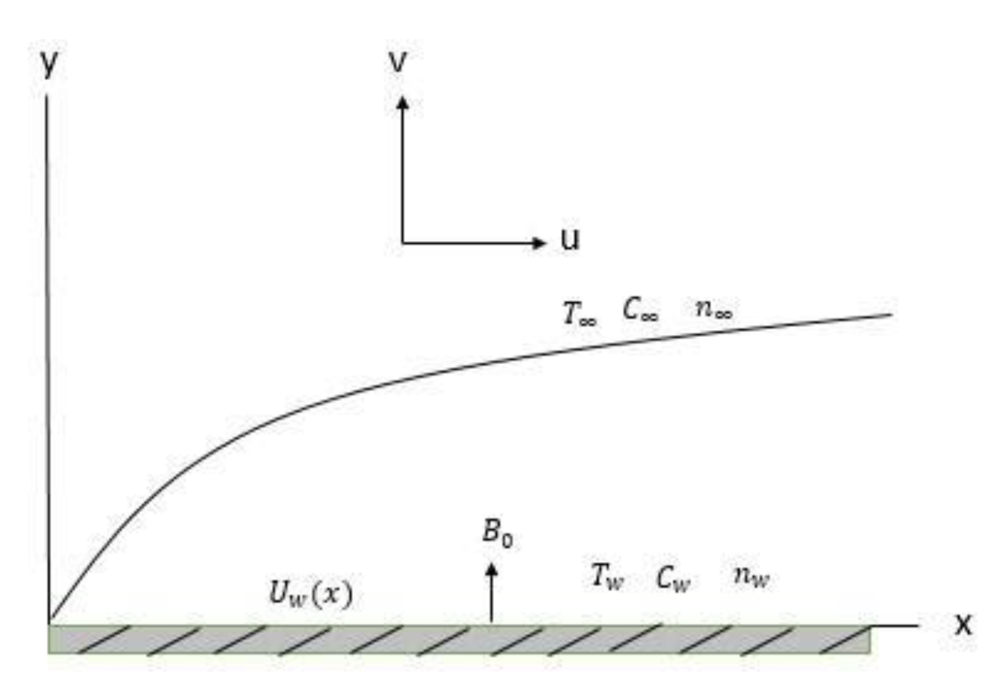
2. Mathematical Modeling

Considering 2D steady, laminar boundary layer dissipative nanofluid flow containing gyrotactic microorganisms through an exponentially stretchable surface, the flow geometry of the investigation is exhibited in Figure 1. Flow formulation is developed by addressing the effectiveness of magnetic field, viscous dissipation, thermophoresis, and Brownian motion. The x and y pivots are considered along the pivotal trend of the exponentially stretchable surface, and perpendicular to y-axis respectively. The stretching velocity, $U_w\left(x\right)$, is presumed to vary as $U_w\left(x\right)=ax$, where $a$ is plus constant. It was also presumed that the constant of temperature, nanoparticle volume fraction, and density of motile microorganisms at the stretchable surface were $T_w$, $C_w$, and $n_w$, respectively; and they were also presumed to be constants far from the stretchable surface $T_{\infty }$, $C_{\infty }$, and $n_{\infty }$, respectively. Velocity components, $u$ and $v$, were taken through the $x$ and $y$ axes, respectively. A constant magnetic strength, B₀, was acted in the y-trend. Note that the flow encouraged by bioconvection occupies a place in elevated nanoparticles suspension, with a view to obtain the release of inhibiting bioconvection. According to these assumptions, the governing equations concerning the present investigation can be addressed as (see Rashad et al. [23], Babu and Sandeep [25], and Khan and Pop [26]);

Continuity equation:

$$\frac{\partial u}{\partial x}+\frac{\partial v}{\partial y}=0.$$

(1)

Momentum equation:

$$u\frac{\partial u}{\partial x}+v\frac{\partial u}{\partial y}=\upsilon \left(\frac{{\partial }^{2}u}{\partial y^2}\right)-\frac{{\sigma }_e{B}_0^2}{\rho }u.$$

(2)

Thermal energy equation:

$$u\frac{\partial T}{\partial x}+v\frac{\partial T}{\partial y}=\alpha \left(\frac{{\partial }^{2}T}{\partial y^2}\right)-\frac{{\sigma }_e{B}_0^2}{\rho }u+\mu {\left(\frac{\partial u}{\partial y}\right)}^2+\tau \left(D_B\left(\frac{\partial T}{\partial y}\frac{\partial C}{\partial y}\right)+\frac{D_T}{T_{\infty }}{\left(\frac{\partial T}{\partial y}\right)}^2\right)$$

(3)

Nanoparticles equation:

$$u\frac{\partial C}{\partial x}+v\frac{\partial C}{\partial y}=D_B\left(\frac{{\partial }^{2}C}{\partial y^2}\right)+\frac{D_T}{T_{\infty }}\left(\frac{{\partial }^{2}T}{\partial y^2}\right).$$

(4)

Conservation equation for microorganisms:

$$u\frac{\partial n}{\partial x}+v\frac{\partial n}{\partial y}-D_n\left(\frac{{\partial }^{2}n}{\partial y^2}\right)+\frac{d{W}_c}{C_w-C_{\infty }}\frac{\partial }{\partial y}\left(n\frac{\partial C}{\partial y}\right)=0.$$

(5)

Subject to:

$$\begin{array}{l}u=U_w,v=0,T=T_w=T_{\infty }+T_0{e}^{x/2L}\hspace{1em}\hspace{1em}\hspace{1em}\mathrm{at}y=0\\ C=C_w=C_{\infty }+C_0{e}^{x/2L},n=n_w=n_{\infty }+n_0{e}^{x/2L}\end{array}$$

(6)

$$u\to 0,T\to T_{\infty },C\to C_{\infty },n\to n_{\infty }\mathrm{as}y\to \infty .$$

(7)

where $T$ stands for the nanofluid temperature. $C$ stands for the nanoparticle volume fraction. $n$ stands for the number density of motile microorganisms. ${\sigma }_e$ stands for the electrical conductivity. $\upsilon$, $\mu$ and $\alpha$ stand for are the kinematic viscosity, dynamic viscosity and thermal diffusivity of the nanofluid. $\rho$ stands for the nanofluid density. $T_0$, $C_0$, and $n_0$ stand for the constants which measure the rate of surface temperature, nanoparticle volume fraction, and density of motile microorganisms, respectively. $D_B$ stands for the Brownian diffusion coefficient. $D_n$ stands for the diffusivity of microorganisms. $W_c$ stands for the maximum cell swimming speed. $D_T$ stands for the thermophoretic diffusion coefficient. $\tau ={\left(\rho c\right)}_p/{\left(\rho c\right)}_f$ stands for the ratio between the effective heat capacity of the nanoparticle material ${\left(\rho c\right)}_p$ and heat capacity of the fluid ${\left(\rho c\right)}_f$. $L$ stands for the sheet length.

The Equations (1) to (7) can be transformed to dimensionless forms by using the following non-dimensional variables (similarity transformations)

$$\begin{array}{l}u=U_w{e}^{x/2L}{f}^{\prime },v=-\sqrt{\frac{\upsilon U_w}{2\upsilon L}}{e}^{x/2L}\left(f+\eta f^{\prime }\right),\psi =\sqrt{2\upsilon U_{w}L}{e}^{x/2L}f\\ \\ \chi (\eta )=\frac{n-n_{\infty }}{n_w-n_{\infty }},\theta (\eta )=\frac{T-T_{\infty }}{T_w-T_{\infty }},\varphi (\eta )=\frac{C-C_{\infty }}{C_w-C_{\infty }},\eta =y\sqrt{\frac{U_w}{2\upsilon L}}{e}^{x/2L},\end{array}$$

(8)

where $\psi$ stands for the stream function determining the continuity equation (Equation (1)). $f(\eta )$ stands for the dimensionless stream function. $f^{\prime }(\eta )$ stands for the dimensionless velocity profile. $\theta (\eta )$ and $\varphi (\eta )$ stand for the dimensionless nanofluid temperature and the nanoparticle volume fraction in the boundary layer region, respectively. $\chi (\eta )$ stands for the dimensionless density of motile microorganisms, and $\eta$ stands for similarity variable or dimensionless coordinate.

By substituting Equation (8) into Equations (1) to (5), the transformed equations are:

$$f^{‴}+f{f}^{″}-2{f^{\prime }}^2-M{f}^{\prime }=0$$

(9)

$${\theta }^{″}+Nb\mathrm{Pr}{\theta }^{\prime }{\varphi }^{\prime }+\mathrm{Pr}f{\theta }^{\prime }+\mathrm{Pr}Nt{{\theta }^{\prime }}^2+\mathrm{Pr}Ec{f^{″}}^2-\mathrm{Pr}{f}^{\prime }\theta =0$$

(10)

$${\varphi }^{″}+Lef{\varphi }^{\prime }+\left(\frac{Nt}{Nb}\right){\theta }^{″}=0$$

(11)

$${\chi }^{″}+2Lb\mathrm{Pr}f{\chi }^{\prime }-Pe\left({\varphi }^{\prime }{\chi }^{\prime }+\chi {\varphi }^{″}+\sigma {\varphi }^{″}\right)=0$$

(12)

The related boundary conditions (6)–(7) become:

$$\begin{array}{l}f=0,f^{\prime }=1,\theta =1,\varphi =1,\chi =1 \mathrm{as} \eta =0,\\ f^{\prime }\to 0,\theta \to 0,\varphi \to 0,\chi \to 0 \mathrm{as} \eta \to \infty ,\end{array}$$

(13)

where prime symbolizes differentiation with regard to $\eta$, the magnetic field parameter $M=\frac{\sigma B_0^2}{\rho a},$ thermophoresis parameter $Nt=\left(\frac{{\left(\rho c\right)}_p{D}_B\left(T_w-T_{\infty }\right)}{\upsilon T_{\infty }{\left(\rho c\right)}_f}\right)$, Brownian motion parameter $Nb=\left(\frac{{\left(\rho c\right)}_p{D}_B\left(C_w-C_{\infty }\right)}{\upsilon T_{\infty }{\left(\rho c\right)}_f}\right)$, Prandtl number $\mathrm{Pr}=\frac{\mu c_p}{\kappa }$, Peclet number $Pe=\frac{d{W}_c}{D_n}$, Lewis number $Le=\frac{\upsilon }{D_B}$, bioconvection Lewis number $Lb=\frac{\alpha }{D_n}$, bioconvection parameter $\sigma =\frac{n_{\infty }}{n_w-n_{\infty }}$, and Eckert number $Ec=\frac{\mu a}{\rho c_p\left(T_w-T_{\infty }\right)}$.

3. Spectral Relaxation Method

In this study, SRM is utilized to solve the transformed differential Equations (9)–(12) according to the boundary conditions (13). Generally, SRM is developed based on modest iteration modes, established by decreasing the order of the momentum equation by reconfiguring the performing governing nonlinear ordinary differential equation systems. SRM also did not need any appraisal of perturbation, derivatives, and linearization, unlike other iterative numerical schemes for solving nonlinear systems of ordinary differential equations (Motsa, [27]). As discussed by Motsa and Makukula [28], SRM is designed for solving a set of coupled nonlinear differential equations where the governing unknown functions have exponentially decaying profiles. For at least one set of related profiles, for example, when velocity profile and temperature profile decays exponentially, SRM is identified as one of the best methods for solving boundary layer problems (Motsa & Makukula [28]). In addition, SRM is preferred in solving the present study due to its great accuracy and for subsequent solutions and discretization of variable-coefficient linear differential equations, with convenient solutions through modest ranges (Motsa & Makukula [28]). In order to discretize the transformed Equations (9)–(12), the following SRM algorithm [27,28,29] is used:

Algorithm 1: Spectral Relaxation Method

Step 1: Introducing the transformation: $f^{\prime }\left(\eta \right)=F\left(\eta \right)$. Step 2: Depict the original equation in terms of $F\left(\eta \right)$ to decrease the order of the momentum equation for $f\left(\eta \right)$ $F\left(\eta \right)$. Step 3: Assume that $F\left(\eta \right)$, $\theta \left(\eta \right)$, $\varphi \left(\eta \right)$, $\chi \left(\eta \right)$ are similar to the former iteration (indicated by $f_r\left(\eta \right)$, ${\theta }_r\left(\eta \right)$, ${\varphi }_r\left(\eta \right)$, and ${\chi }_r\left(\eta \right)$). Step 4: Construct an iteration scheme for $F\left(\eta \right)$, $\theta \left(\eta \right)$, $\varphi \left(\eta \right)$, and $\chi \left(\eta \right)$. Step 5: Assume that only linear terms in $F\left(\eta \right)$, $\theta \left(\eta \right)$, $\varphi \left(\eta \right)$, and $\chi \left(\eta \right)$ are to be estimated at the present iteration scale (indicated by $F_{r+1}\left(\eta \right)$, ${\theta }_{r+1}\left(\eta \right)$, ${\varphi }_{r+1}\left(\eta \right)$, ${\chi }_{r+1}\left(\eta \right)$), and all other terms are presumed to be similar to the former iteration.

It is worth noting that the above strategy is similar to the Gauss–Seidel method for decoupling linear algebraic systems of equations. After applying the previous algorithm, a series of linear differential equations (DE) with constant coefficients are generated, which can be solved by using Chebyshev spectral collocation patterns. Spectral patterns are chosen due to their high accuracy and can give smooth solutions over simple domains. After applying the previous algorithm, Equations (9)–(13) became:

$${f^{‴}}_{r+1}+f_r{f^{″}}_{r+1}-2{f^{\prime }}_r{}^2-M{f^{\prime }}_{r+1}=0$$

(14)

$${{\theta }^{″}}_{r+1}+Nb\mathrm{Pr}{{\theta }^{\prime }}_{r+1}{{\varphi }^{\prime }}_r+\mathrm{Pr}{f}_{r+1}{{\theta }^{\prime }}_{r+1}+\mathrm{Pr}Nt{{\theta }^{\prime }}_r{}^2+\mathrm{Pr}Ec{f^{″}}_{r+1}{}^2-\mathrm{Pr}{f^{\prime }}_{r+1}{\theta }_{r+1}=0$$

(15)

$${{\varphi }^{″}}_{r+1}+Le{f}_{r+1}{{\varphi }^{\prime }}_{r+1}+\left(\frac{Nt}{Nb}\right){{\theta }^{″}}_{r+1}=0$$

(16)

$${{\chi }^{″}}_{r+1}+2Lb\mathrm{Pr}{f}_{r+1}{{\chi }^{\prime }}_{r+1}-Pe\left({{\varphi }^{\prime }}_{r+1}{{\chi }^{\prime }}_{r+1}+{\chi }_{r+1}{{\varphi }^{″}}_{r+1}+\sigma {{\varphi }^{″}}_{r+1}\right)=0$$

(17)

$$\begin{array}{l}{F}_{r+1}\left(0\right)=1;F_{r+1}(\infty )=0\\ {\theta }_{r+1}\left(0\right)=1;{\theta }_{r+1}(\infty )=0\\ {\varphi }_{r+1}\left(0\right)=1;{\varphi }_{r+1}(\infty )=0\\ {\chi }_{r+1}\left(0\right)=1;{\chi }_{r+1}(\infty )=0\end{array}$$

Utilizing the Chebychev spectral collocation technique we get:

$$A_1{F}_{r+1}=B_1$$

$$A_2{F}_{r+1}=B_2$$

$$A_3{\theta }_{r+1}=B_3$$

$$A_4{\varphi }_{r+1}=B_4$$

$$A_5{\chi }_{r+1}=B_5$$

where,

$$A_1=D^2+diag\left[f_r\right]D-MI$$

$$B_1=2{F^{\prime }}_r$$

$$A_2=D$$

$$B_2=F_{r+1}{A}_3=D^2+diag\left[Nb\mathrm{Pr}{{\varphi }^{\prime }}_r+\mathrm{Pr}{f}_{r+1}\right]D-\mathrm{Pr}diag\left[F\right]$$

$$B_3=-\mathrm{Pr}Nt{{\theta }^{\prime }}_r{}^2-\mathrm{Pr}Ec{F^{\prime }}^2$$

$$A_4=D^2+diag\left[Le{f}_r\right]D$$

$$B_4=-\frac{Nt}{Nb}{{\theta }^{″}}_{r+1}$$

$$A_5=D^2+diag\left[2Lb\mathrm{Pr}{f}_{r+1}-Pe{{\varphi }^{\prime }}_{r+1}\right]D-Pediag\left[{{\varphi }^{″}}_{r+1}\right]$$

$$B_5=Pe\sigma {{\varphi }^{″}}_{r+1}$$

4. Results and Discussion

In this segment, we have converted the governing Equations (2)–(5) with boundary conditions (6)–(7) employing proper similarity variables, and obtained the converted Equations (9)–(12) with boundary condition (13). Therefore, the data are revealed in graphical form for various values of parameters, such as thermophoresis parameter, $Nt$; Brownian motion parameter, $Nb$; magnetic field parameter, $M$; Peclet number, $Pe$; Prandtl number, $\mathrm{Pr}$; bioconvection Lewis number, $Lb$; Lewis number, $Le$; and bioconvection constant, $\sigma$. To confirm the obtained outcomes, the current outcomes for of local Nusselt number $-{\theta }^{\prime }\left(0\right)$ were compared with those gained by Bidin and Nazar [30] for the status of viscous fluid by putting $Nt=Nb=Le=Lb=Pe=M=Ec=\sigma =0$ in Equations (9)–(12) and neglecting the Eckert number, $Ec$, and radiation number, $K$, i.e., by setting $Ec=0$ and $K=0$ in Equation (10) of that paper. The comparison results are also validated by using the boundary value problem solver (bvp4c) in MATLAB software. In

Table 1. Comparison of of local Nusselt number $-{\theta }^{\prime }\left(0\right)$ for various values of $\mathrm{Pr}$ for $Nt=Nb=Le=Lb=Pe=M=Ec=\sigma =0$.

Pr	Bidin and Nazar [30]	Magyari and Keller [31]	El-Aziz [32]	Loganthan and Vimala [33]	Present Study
					SRM	Bvp4c
1	0.9547	0.954782	0.954785	0.954955	0.9548	0.954782
1.5					1.2348	1.234755
2	1.4714				1.4715	1.471460
2.5					1.6802	1.680229
3	1.8691	1.869075	1.869074	1.869074	1.8691	1.869073
5		2.500135	2.500132	2.500184	2.5001	2.500131
7					3.0133	3.013277
10		3.660379	3.660372	3.660379	3.6604	3.660372
20					5.3016	5.301625

, the values of local Nusselt number $-{\theta }^{\prime }\left(0\right)$ were compared with those performed by Magyari and Keller [31], El-Aziz [32], and Loganthan and Vimala [33] for the case of magneto-nanofluid flow through a permeable exponentially radiating stretchable surface in a stratified medium. The comparison was performed by removing the gyrotactic microorganisms (by removing Equation (12)) and putting the magnetic parameter, $M=0$; the stratification parameter, $St=0$; the radiation parameter, $Nr=0$; the suction parameter, $f_w=0$; and volume fraction, $\varphi =0$, in Equations (12) to (14) of the paper by Loganthan and Vimala [33]. The comparisons, as indicated in Table 1, exhibit an excellent agreement, thus giving certainty to the outcomes that will be performed for the bioconvection case. We used the SRM technique to discretize our converted Equations (13) to (17) and used MATLAB to get our demand data. In this study, numerical solutions are obtained for the various values of governing parameters used, especially for Eckert number, $Ec=0.01$, and the Brownian motion parameter, $Nb>0$, which is calculated and fixed throughout this problem.

Figure 2, Figure 3, Figure 4 and Figure 5 are designed to scrutinize the effectiveness of magnetic parameter, $M$, on the nanofluid, velocity, temperature, nanoparticle volume fraction, and density of the motile microorganism curves. It is evident from Figure 2 that escalating estimations of magnetic field strength decreases the velocity profile. This is because the magnetic field is based on Lorentz force theorem. M means more impact between the fluid atoms, which yields more resistive force to fluid flow. In detail, magnetic field effect develops a resistance force, also known as Lorentz force, which works obverse to flow range (see Figure 2) and indirectly promotes the thermal boundary layer thickness, as depicted in Figure 3. As a result, the greater reversing force decreases the fluid flow, and the velocity field declines. It was also seen that the magnetic parameter assists in improving the temperature and volume fraction near the surface, and the thermal and nanoparticle concentration boundary layer thicknesses, as shown in Figure 3 and Figure 4. These observations may occur because of the manifestation of additional heat to the flow to increase the magnetic parameter, M. Therefore, the temperature, concentration, and gyrotactic microorganism boundary layer escalate with larger M, as depicted in Figure 3, Figure 4 and Figure 5.

Figure 6, Figure 7 and Figure 8 revealed the effectiveness of Prandtl number, Pr, on the temperature, nanoparticle fraction, and density of the motile microorganism curves. From Equation (9), it was noted that the velocity was not affected by Prandtl number. It was seen that the temperature and its thermal boundary layer thickness declined with the boost in Pr, as illustrated in Figure 6. Physically, as Pr was boosted, the thermal diffusivity declined, and consequently led to the reduction in the ability of energy that declined the thermal boundary layer. As elucidated in Figure 7, it was noticed that the concentration boundary layer thicknesses were increased with the boost in Pr. Figure 8 was sketched to see the influence of the Pr on the density of motile microorganisms ($\chi (\eta )$). It was noted that the density of motile microorganisms increased with the raise in Pr. It was characterized that the motile microorganism came down for higher Pr because their boundary layer thicknesses scaled down for larger Pr. In other words, the amount of gyrotactic microorganisms reduced due to the growth in Pr.

Variation in thermophoresis parameter ($Nt$) on the temperature and nanoparticle fraction curves are demonstrated in Figure 9 and Figure 10. It was found from Figure 9 and Figure 10, that the thermophoresis parameter, Nt, strongly enhanced both the temperature and nanoparticle fraction. Physically, this phenomenon occurs because thermophoresis parameter raises the density of the thermal boundary layer. Therefore, temperature increases with the increase in thermophoresis parameter, as shown in Figure 9. In detail, the upsurge in $Nt$ causes an escalation in both the temperature and nanoparticle volume fraction curves. Physically, in thermophoresis phenomena, the tiny particles of the fluid are pulled back from the warm to cold area. Then, the particles of the nanofluid move back from the surface, which is heated, and consequently temperature, thermal boundary layer, and nanoparticle volume fraction profiles are enhanced. Ultimately, the velocity and density of the motile microorganism curves are not influenced by $Nt$.

Figure 11 and Figure 12 presented the impact of Brownian motion parameter, $Nb$, on the temperature and nanoparticle volume fraction curves. It was observed that as $Nb$ upsurges, the temperature boundary layer was enhanced and the opposite happens with the nanoparticle volume fraction boundary thickness. From Figure 12, Brownian motion parameter lessens the concentration boundary layer thickness, which contributes to a decline in concentration. Another physical explanation for this situation is that the greater Brownian motion results in an arbitrary movement of the particles. Due to this arbitrary movement, extra heat is produced. Thus, the growth in temperature curves was explored. Moreover, both velocity and density of the motile microorganism profiles were not influenced by $Nb$. In additon, both the Nusselt number and shear stress were not affected by $Le$, so the velocity and temperature curves were also not influenced.

From Figure 13 and Figure 14, it was seen that the upsurge in $Le$ created a depression in the concentration profile, while the opposite was observed with the microorganism profile at $\eta \approx 1.2$, as manifested in Figure 14. In the effective area, $\eta <1.2$, the growth in $Le$ produced a decrease in the microorganism boundary layers. Additionally, for $\eta >1.2$, the opposite took place as $Le$ grew. From Figure 13, it was clear that the concentration dwindled with the increments of $Le$. Physically, $Le$ decreased the mass diffusivity and as a result, minimizes the permeation depth of the boundary layer.

Figure 15, Figure 16 and Figure 17 indicated that the decline in the boundary layer thickness of density motile microorganisms due to the growth in the bioconvection Lewis number, $Lb$; bioconvection parameter, $\sigma$; and Peclet number, $Pe$. Figure 18 exhibits the residual errors of Equations (13)–(17) versus iterations for several rates of parameters. The residual errors of $f\left(\eta \right)$, $\theta \left(\eta \right)$, $\varphi \left(\eta \right)$, and $\chi \left(\eta \right)$ gathers linear forms. The velocity, temperature, nanoparticles fraction, and motile microorganism profiles shown in Figure 2, Figure 3, Figure 4, Figure 5, Figure 6, Figure 7, Figure 8, Figure 9, Figure 10, Figure 11, Figure 12, Figure 13, Figure 14, Figure 15, Figure 16 and Figure 17 determine the far field boundary conditions (13) asymptotically, which leads to the confidence of the present outcomes.

5. Conclusions

Extensive numerical investigation was performed for two dimensional MHD steady flow, and heat and mass transfer of dissipative nanofluid containing gyrotactic microorganisms over an exponentially stretchable surface. The impacts of thermophoresis, Brownian diffusion, and magnetic field were addressed. In this investigation, the effectiveness of the magnetic strength, the thermophoresis parameter, and the Brownian motion parameter on the MHD bioconvection of nanofluid through a stretchable surface was discussed. The following conclusions were drawn from the finding of this numerical investigation:

• The comparison values of heat rate transfer were in good agreement with the former study, and hence led to the confidence of the present results to be reported further.
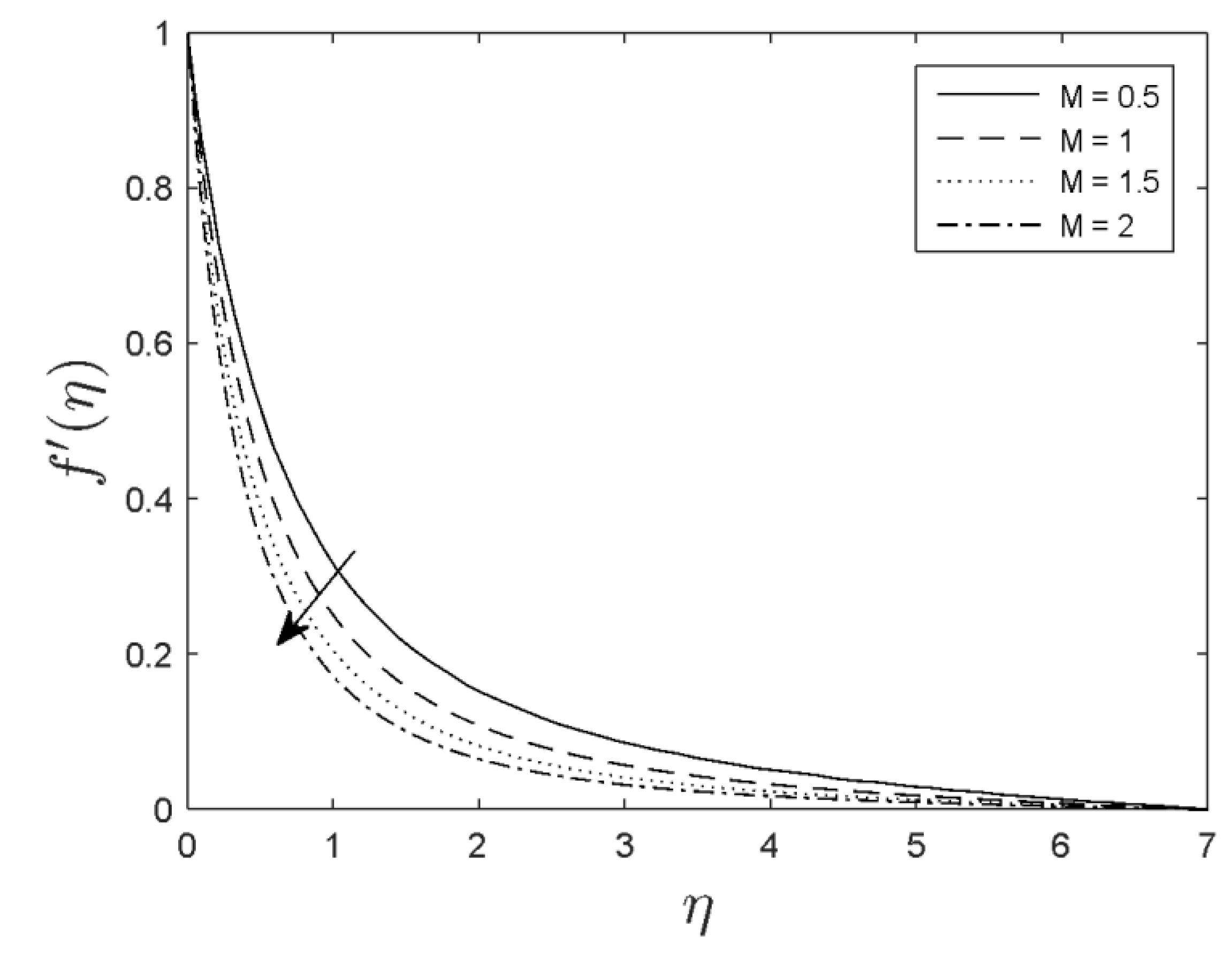
• The resultant velocity diminished with the increments in the magnetic parameter.
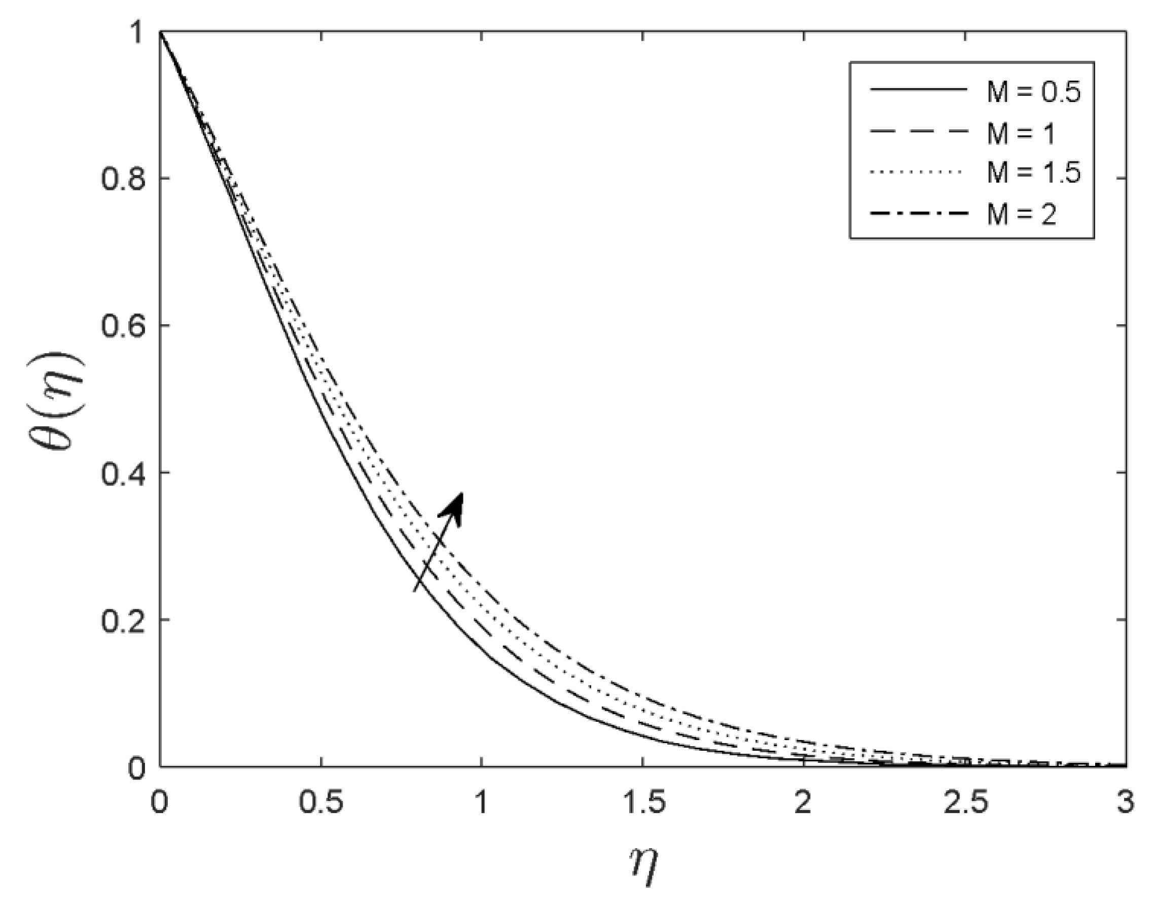
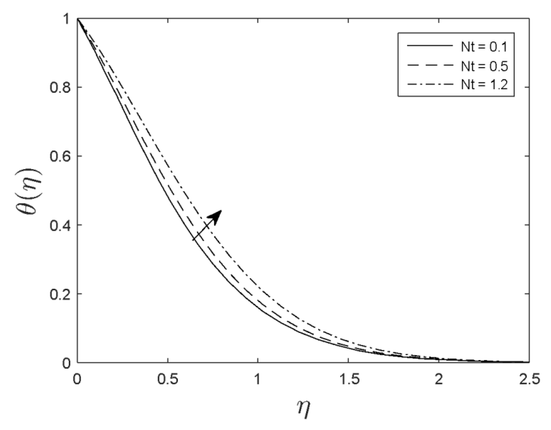
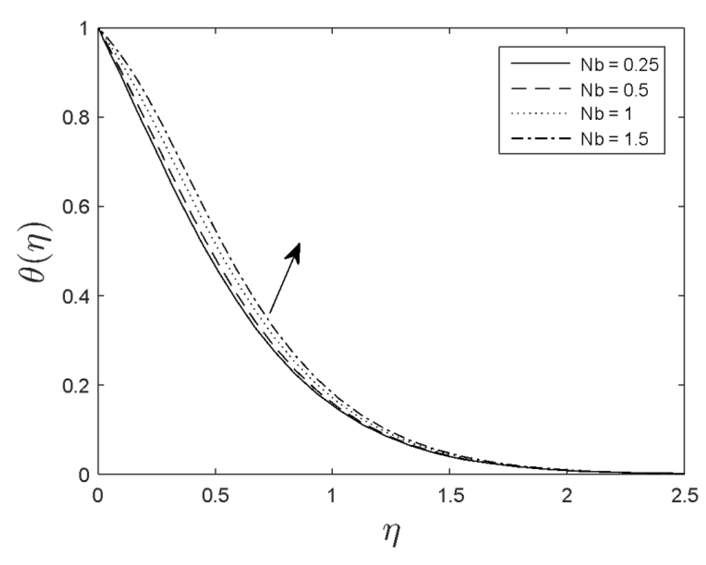
• Fluid temperature increased as the magnetic parameter, thermophoresis, and Brownian motion parameters increased.
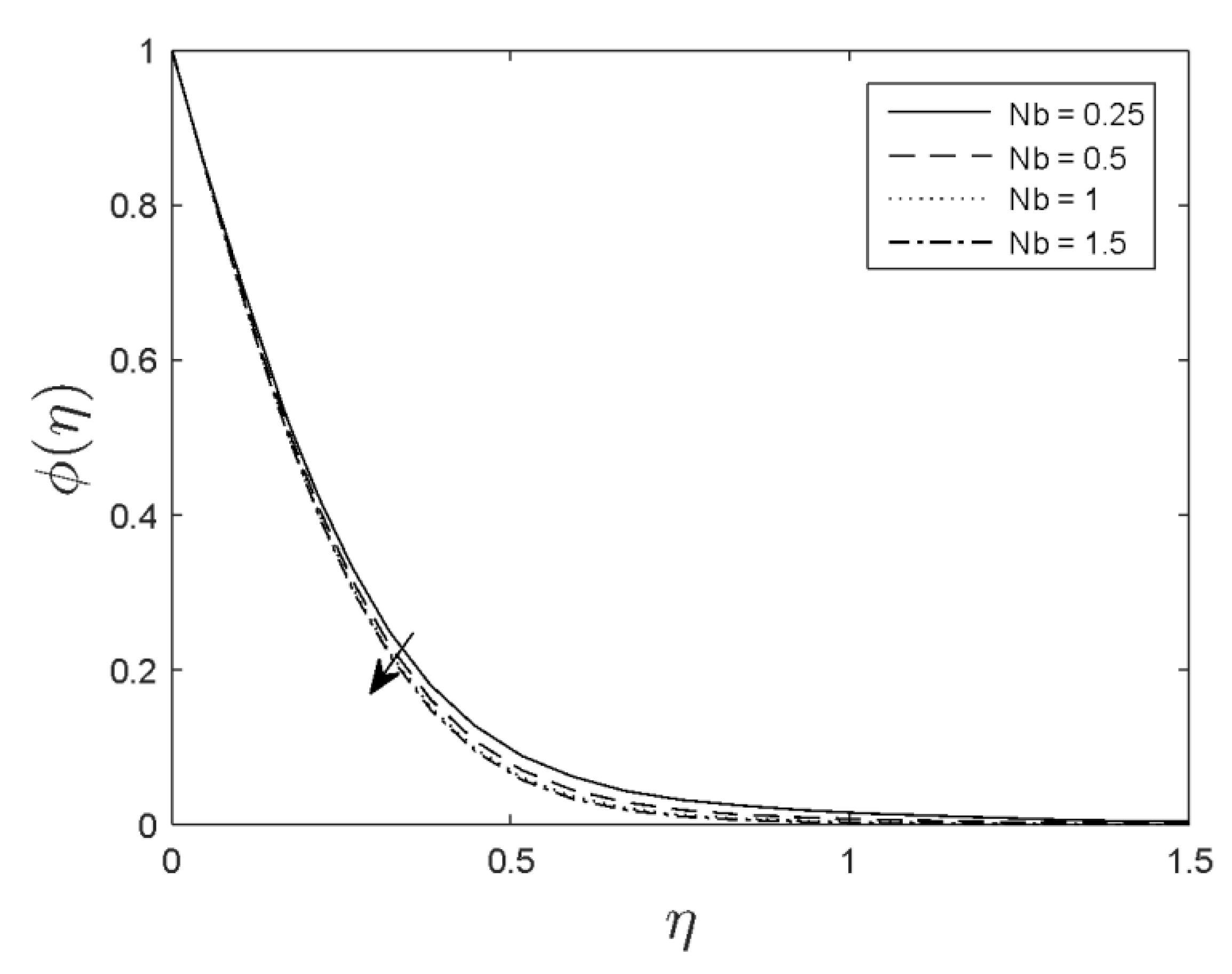
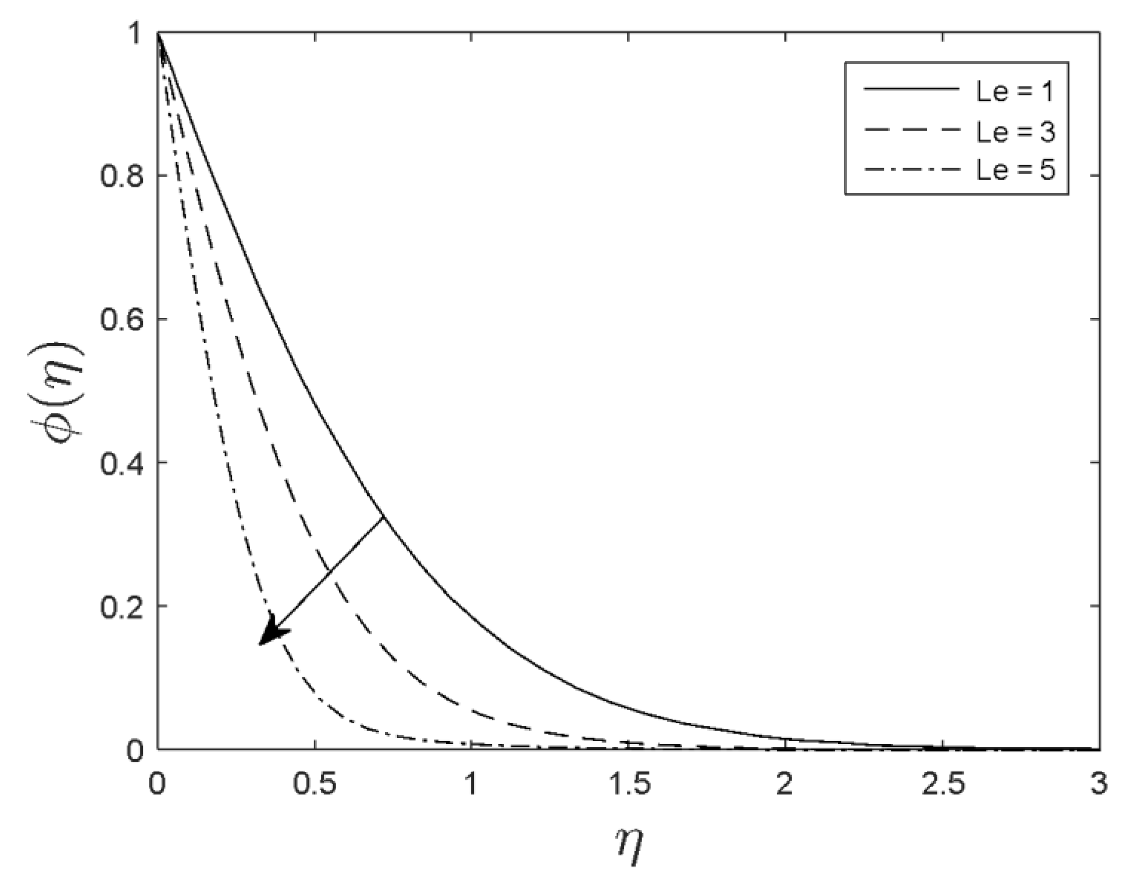
• The concentration was reduced with the boost in the Lewis number and Brownian motion parameter.
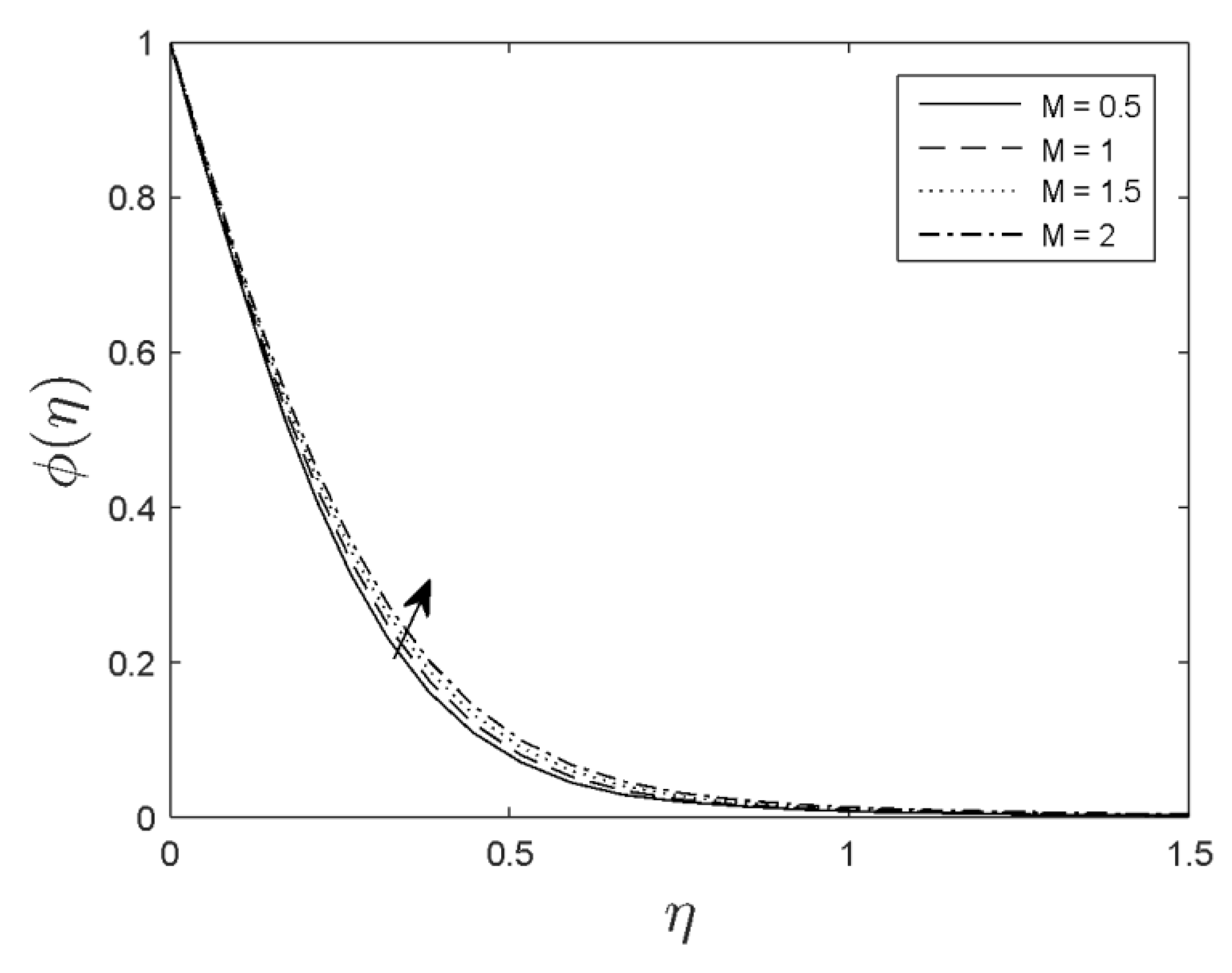
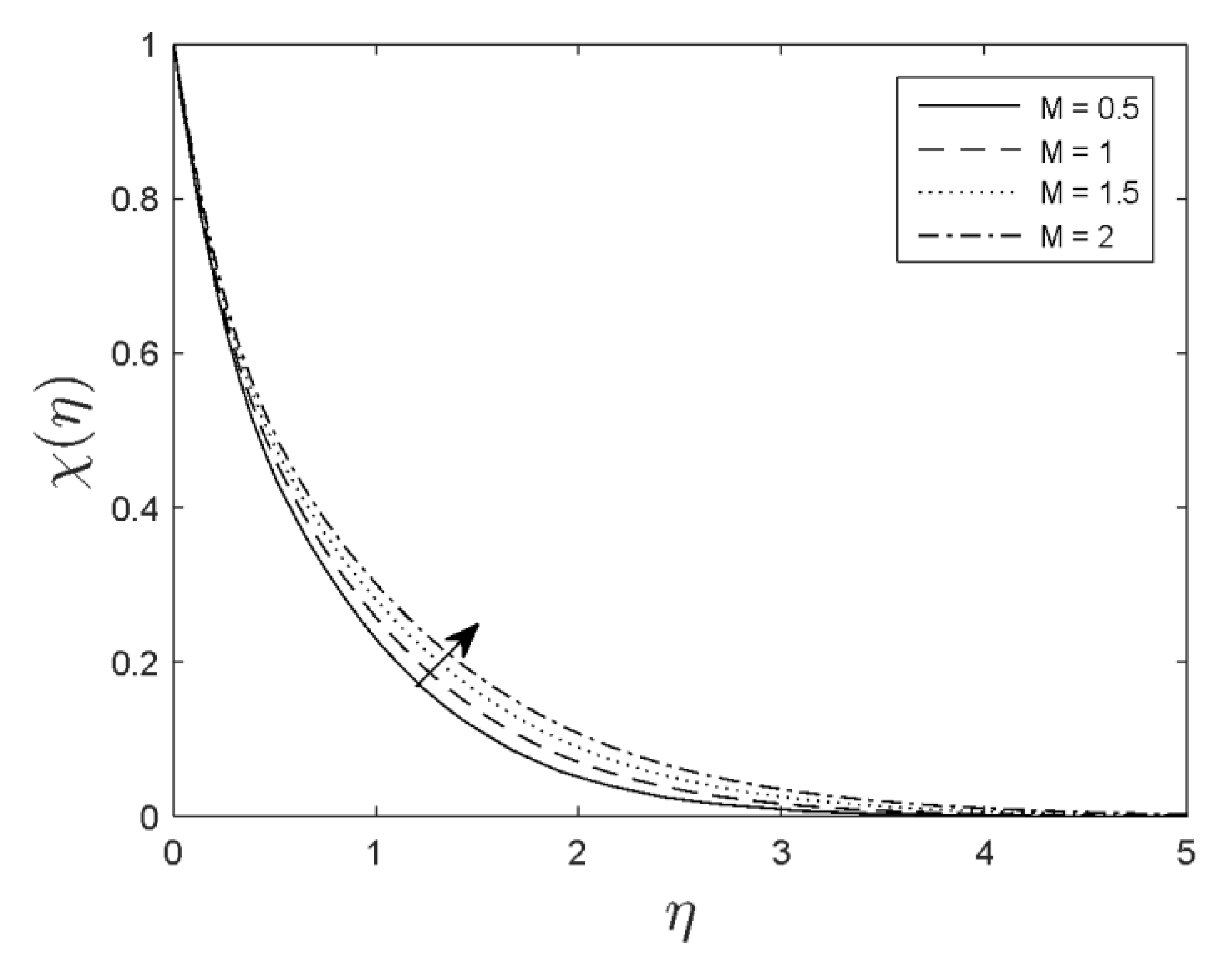
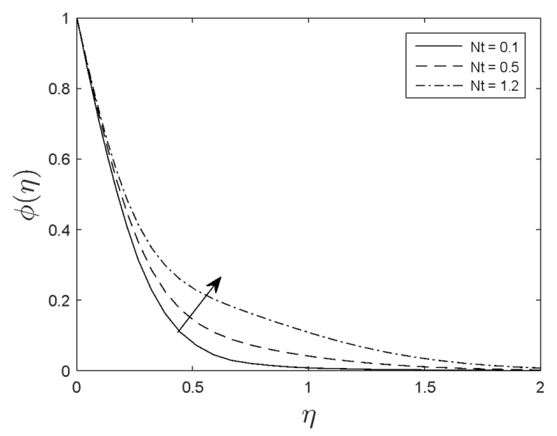
• The concentration was increased with the increment in the Prandtl number, thermophoresis, and magnetic parameters.
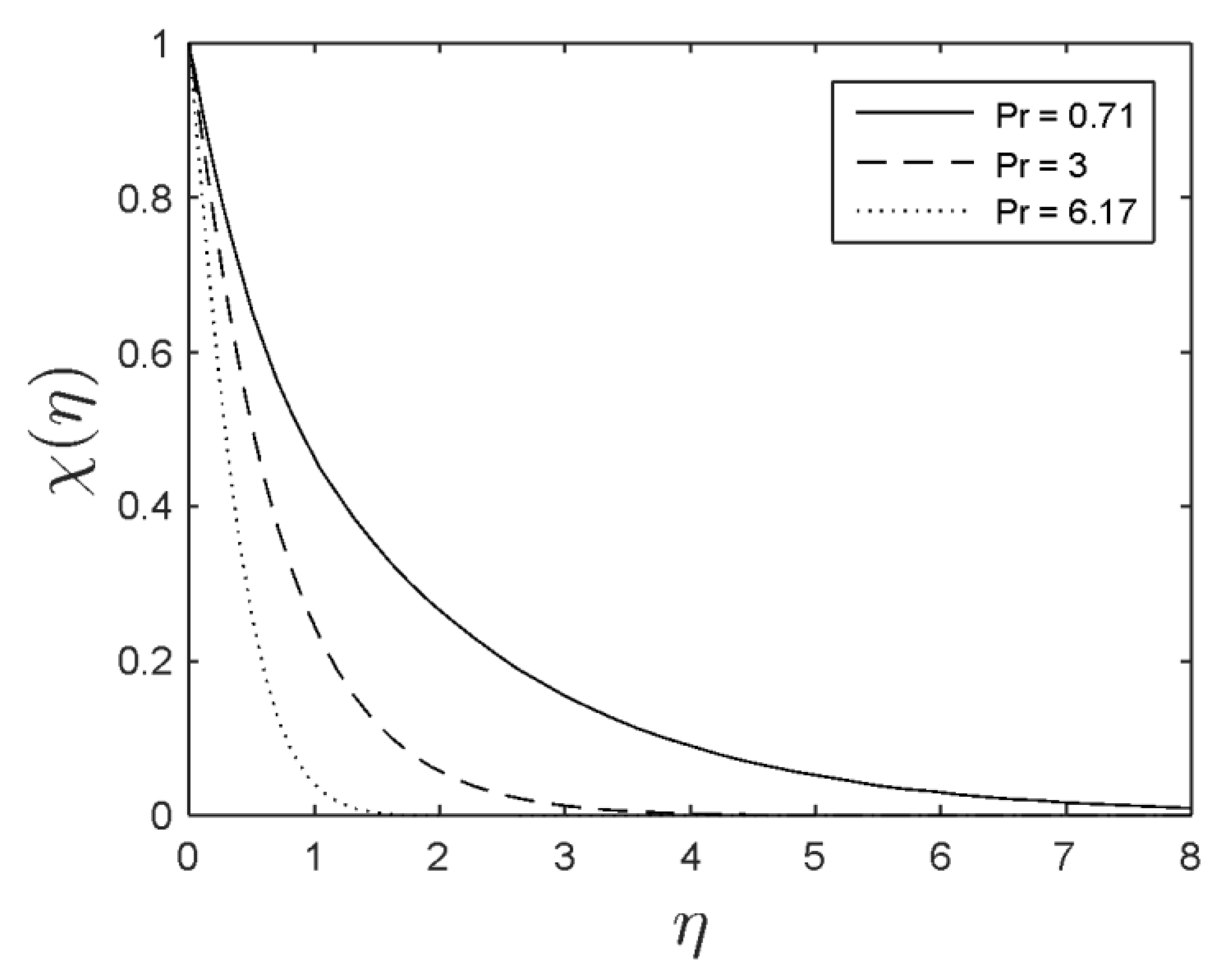
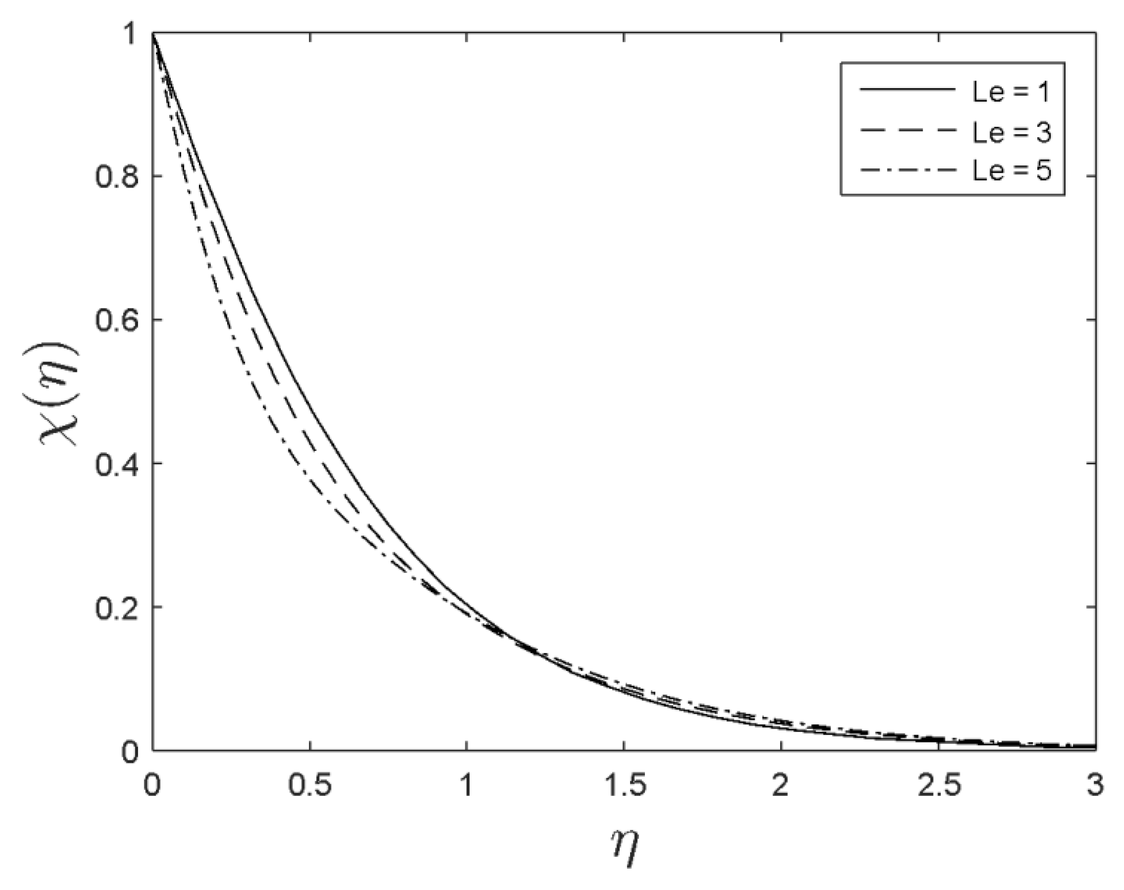
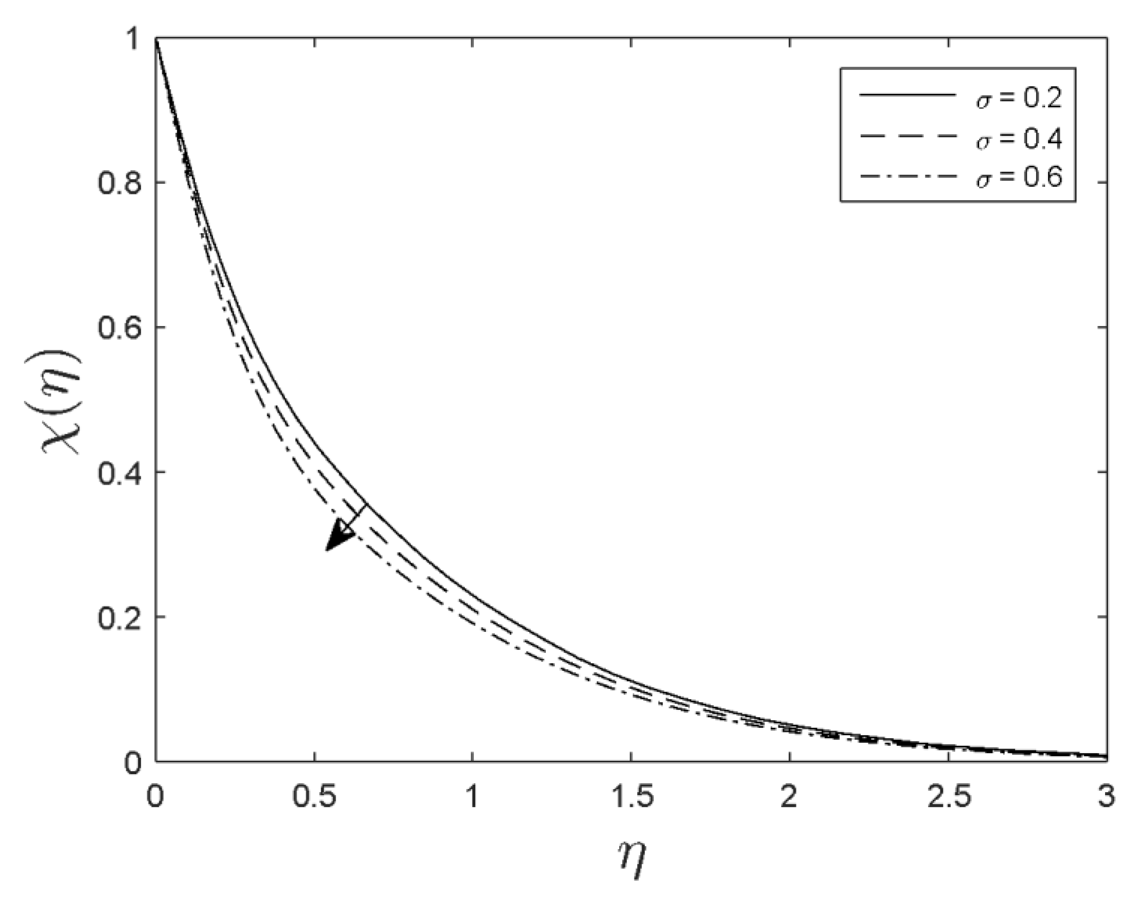
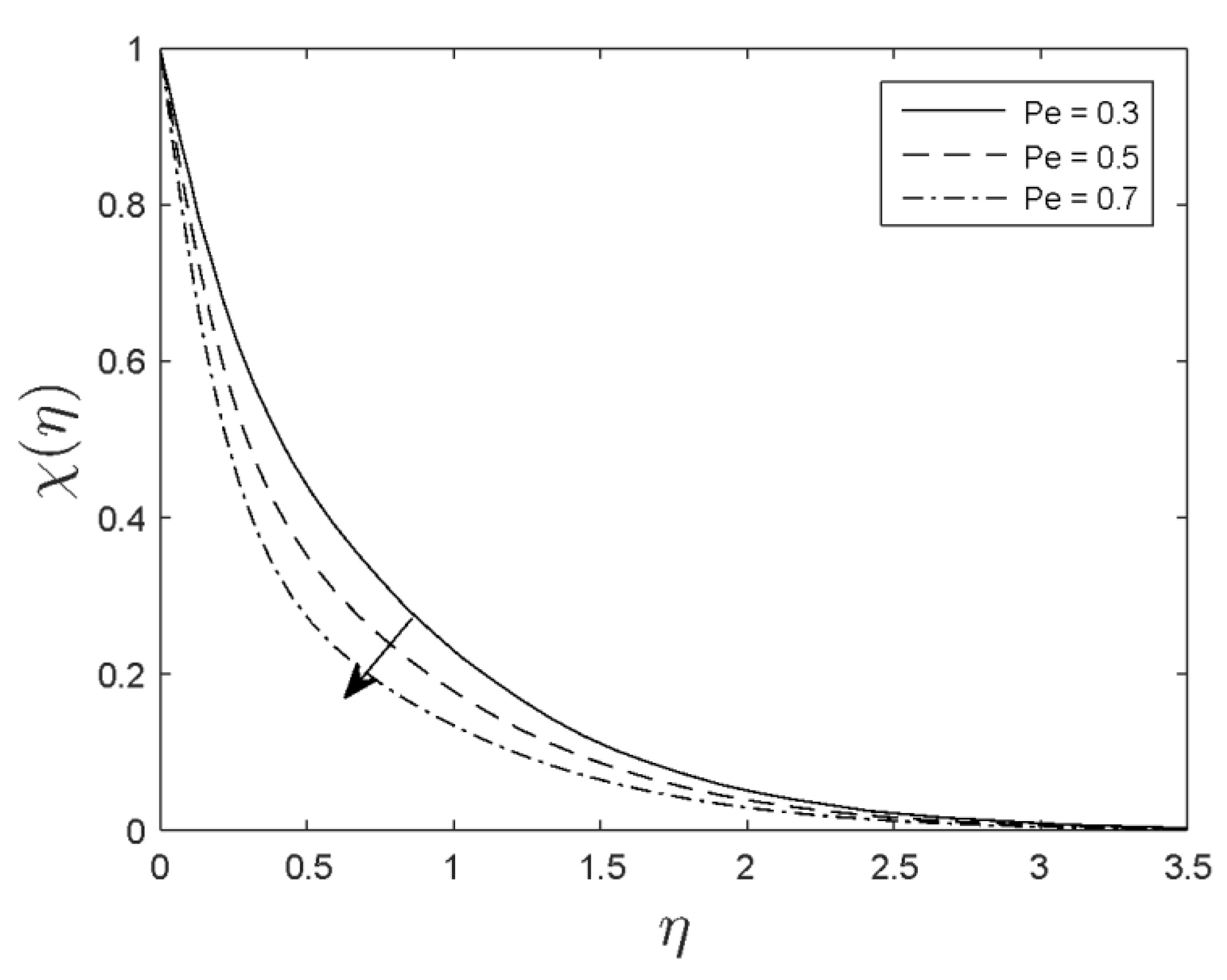
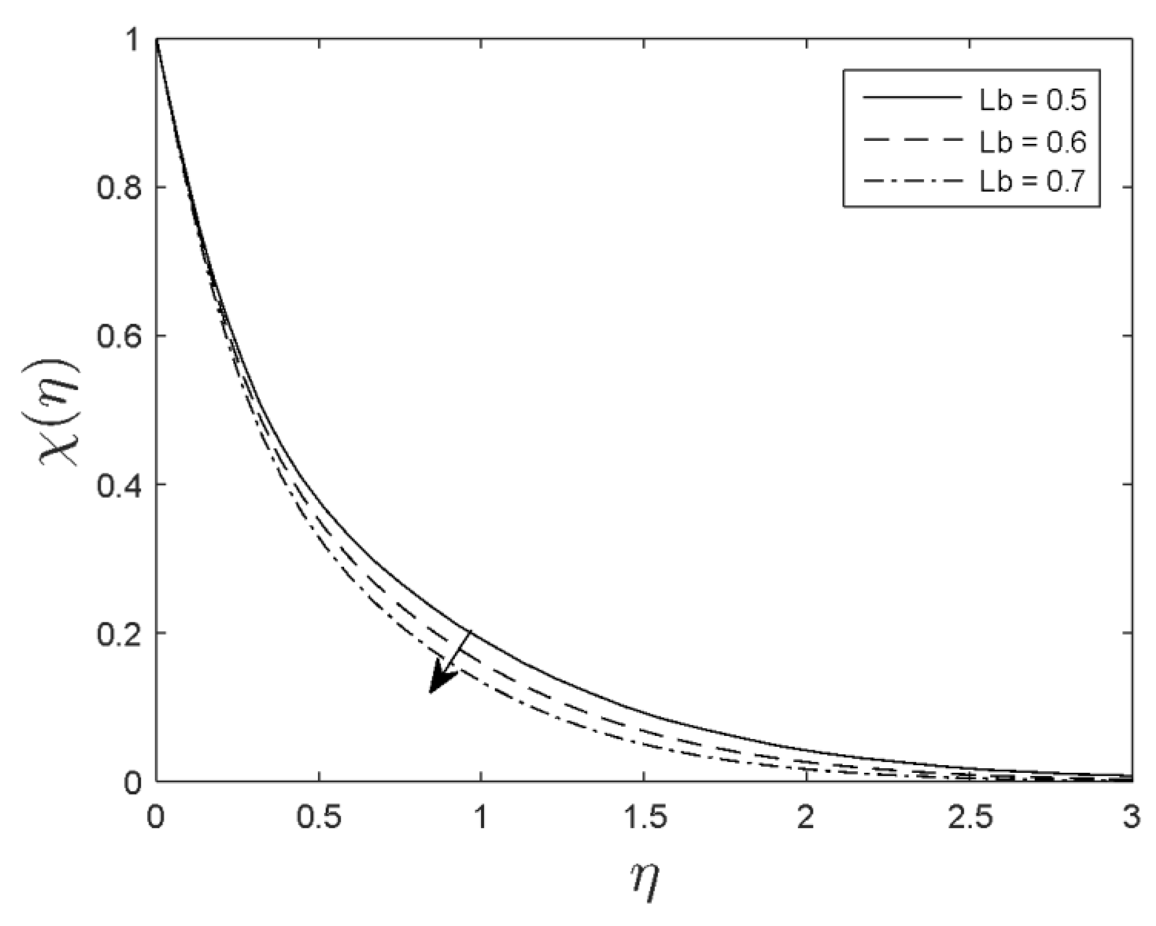
• The density of the motile microorganism is a decreasing function of the Prandtl number, Lewis number, Peclet number, bioconvection Lewis number, and bioconvection parameter.
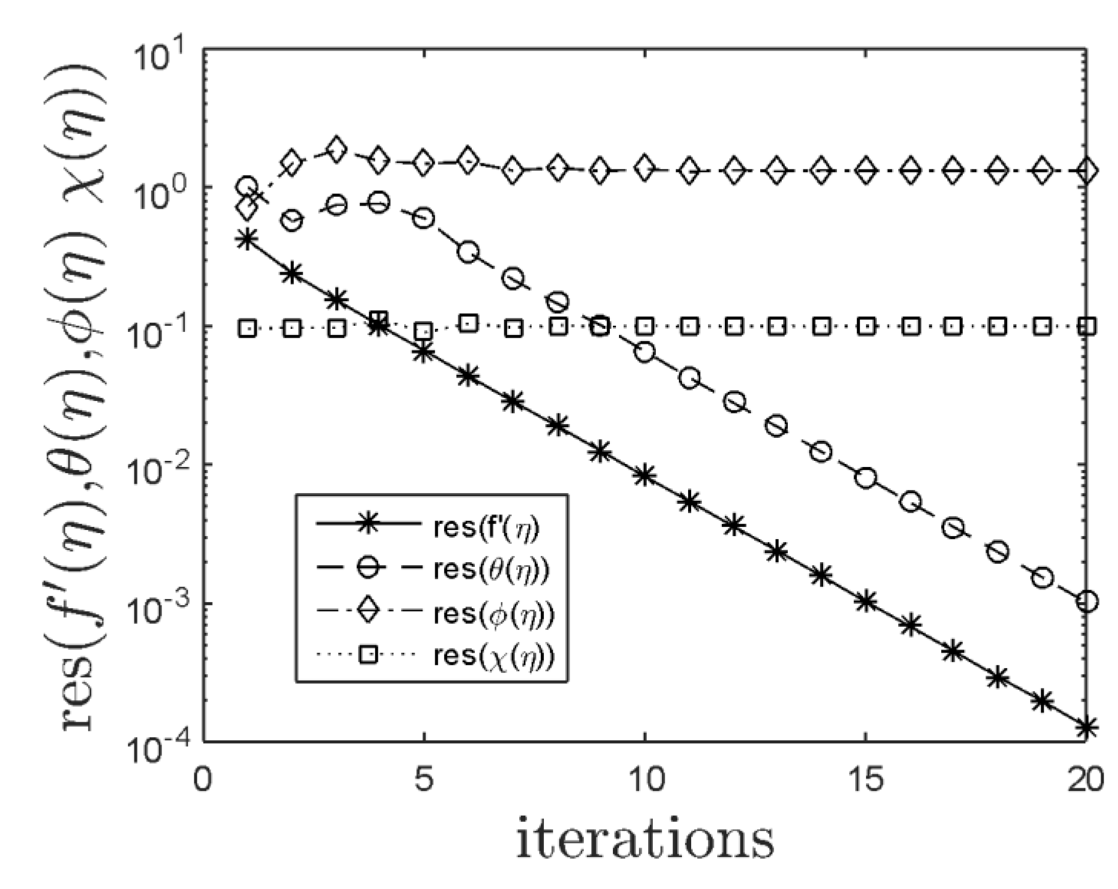
• The residual errors of $f\left(\eta \right)$, $\theta \left(\eta \right)$, $\varphi \left(\eta \right)$, and $\chi \left(\eta \right)$ were iteration dependent.
• For future research, it is suggested for the present study to consider all possible multiple solutions or dual solutions. This is driven by the fact that the multiple solutions cannot be seen experimentally and can only be obtained by using numerical simulation.
• It was also proposed for the stability of multiple solutions to be included as one of the main objective studies for future work. Stability analysis is important for identifying the reliability of the multiple solutions, which depend on the assumptions of the physical model.

References

1. Choi, S.U.S.; Singer, D.A.; Wang, H.P. Developments and applications of non-Newtonian flows. ASME Fed. 1995, 66, 99–105. [Google Scholar]
2. Hadavand, M.; Yousefzadeh, S.; Akbari, O.A.; Pourfattah, F.; Nguyen, H.M.; Asadi, A. A numerical investigation on the effects of mixed convection of Ag-water nanofluid inside a sim-circular lid-driven cavity on the temperature of an electronic silicon chip. Appl. Therm. Eng. 2019, 162, 114298. [Google Scholar] [CrossRef]
3. Pourfattah, F.; Arani, A.A.A.; Babaie, M.R.; Nguyen, H.M.; Asadi, A. On the thermal characteristics of a manifold microchannel heat sink subjected to nanofluid using two-phase flow simulation. Int. J. Heat Mass Transf. 2019, 143, 118518. [Google Scholar] [CrossRef]
4. Bazdar, H.; Toghraie, D.; Pourfattah, F.; Akbari, O.A.; Nguyen, H.M.; Asadi, A. Numerical investigation of turbulent flow and heat transfer of nanofluid inside a wavy microchannel with different wavelengths. J. Therm. Anal. Calorim. 2020, 139, 2365–2380. [Google Scholar] [CrossRef]
5. Asadi, A.; Pourfattah, F.; Szilágyi, I.M.; Afrand, M.; Żyłag, G.; Ahn, H.S.; Wongwises, S.; Nguyen, H.M.; Arabkoohsar, A.; Mahian, O. Effect of sonication characteristics on stability, thermophysical properties, and heat transfer of nanofluids: A comprehensive review. Ultrason. Sonochem. 2019, 58, 104701. [Google Scholar] [CrossRef]
6. Asadi, A.; Aberoumand, S.; Moradikazerouni, A.; Pourfattah, F.; Żyła, G.; Estellé, P.; Mahian, O.; Wongwises, S.; Nguyen, H.M.; Arabkoohsar, A. Recent advances in preparation methods and thermophysical properties of oil-based nanofluids: A state-of-the-art review. Powder Technol. 2019, 352, 209–226. [Google Scholar] [CrossRef]
7. Alarifi, I.M.; Nguyen, H.M.; Bakhtiyari, A.N.; Asadi, A. Feasibility of ANFIS-PSO and ANFIS-GA Models in Predicting Thermophysical Properties of Al2O3-MWCNT/Oil Hybrid Nanofluid. Materials 2019, 12, 3628. [Google Scholar] [CrossRef] [Green Version]
8. Asadi, A.; Alarifi, I.M.; Ali, V.; Nguyen, H.M. An experimental investigation on the effects of ultrasonication time on stability and thermal conductivity of MWCNT-water nanofluid: Finding the optimum ultrasonication time. Ultrason. Sonochem. 2019, 58, 104639. [Google Scholar] [CrossRef]
9. Nabwey, H.A.; Boumazgour, M.; Rashad, A.M. Group method analysis of mixed convection stagnation-point flow of non-Newtonian nanofluid over a vertical stretching surface. Indian J. Phys. 2017, 91. [Google Scholar] [CrossRef]
10. Tlili, I.; Nabwey, H.A.; Ashwinkumar, G.P.; Sandeep, N. 3-D magnetohydrodynamic AA7072-AA7075/methanol hybrid nanofluid flow above an uneven thickness surface with slip effect. Sci. Rep. 2020, 10, 1–13. [Google Scholar] [CrossRef] [Green Version]
11. Chamkha, A.J.; Rashad, A.M.; Alsabery, A.I.; Abdelrahman, Z.M.A.; Nabwey, H.A. Impact of Partial Slip on Magneto-Ferrofluids Mixed Convection Flow in Enclosure. J. Therm. Sci. Eng. Appl. 2020, 12, 051002. [Google Scholar] [CrossRef]
12. Ferdows, M.; Nabwey, H.A.; Rashad, A.M.; Uddin, M.J.; Alzahrani, F. Boundary layer flow of a nanofluid past a horizontal flat plate in a Darcy porous medium: A Lie group approach. Proc. Inst. Mech. Eng. Part C J. Mech. Eng. Sci. 2019. [Google Scholar] [CrossRef]
13. Nabwey, H.A.; El-Mky, H.A. Lie group analysis of thermophoresis on a vertical surface in a porous medium. J. King Saud Univ.-Sci. 2019, 31, 1048–1055. [Google Scholar] [CrossRef]
14. Mahdy, A.E.N.; Hady, F.M.; Nabwey, H.A. Unsteady homogeneous-heterogeneous reactions in MHD nanofluid mixed convection flow past a stagnation point of an impulsively rotating sphere. Therm. Sci. 2019, 388. [Google Scholar] [CrossRef]
15. Nabwey, H.A.; EL-Kabeir, S.M.M.; Rashad, A.M. Lie group analysis of effects of radiation and chemical reaction on heat and mass transfer by unsteady slip flow from a non-isothermal stretching sheet immersed in a porous medium. J. Comput. Theor. Nanosci. 2015, 12, 4056–4062. [Google Scholar] [CrossRef]
16. Platt, J.R. Bioconvection Patterns in Cultures of Free-Swimming Organisms. Science 1961, 133, 1766–1767. [Google Scholar] [CrossRef]
17. Pedley, T.J.; Hill, N.A.; Kessler, J.O. The growth of bioconvection patterns in a uniform suspension of gyrotactic micro-organisms. J. Fluid Mech. 1988, 195, 223–237. [Google Scholar] [CrossRef] [Green Version]
18. Kuznetsov, A.V. Bio-thermal convection induced by two different species of microorganisms. Int. Commun. Heat Mass Transf. 2011, 38, 548–553. [Google Scholar] [CrossRef]
19. Alloui, Z.; Nguyen, T.H.; Bilgen, E. Bioconvection of gravitactic microorganisms in a vertical cylinder. Int. Commun. Heat Mass Transf. 2005, 32, 739–747. [Google Scholar] [CrossRef]
20. Uddin, M.J.; Kabir, M.N.; Bég, O.A. Computational investigation of Stefan blowing and multiple-slip effects on buoyancy-driven bioconvectionnanofluid flow with microorganisms. Int. J. Heat Mass Transf. 2016, 95, 116–130. [Google Scholar] [CrossRef]
21. Dhanai, R.; Rana, P.; Kumar, L. Lie group analysis for bioconvection MHD slip flow and heat transfer of nanofluid over an inclined sheet: Multiple solutions. J. Taiwan Inst. Chem. Eng. 2016, 66. [Google Scholar] [CrossRef]
22. Chamkha, A.J.; Rashad, A.M.; Kameswaran, P.K.; Abdou, M.M.M. Radiation effects on natural bioconvection flow of a nanofluid containing gyrotactic microorganisms past a vertical plate with streamwise temperature variation. J. Nanofluids 2017, 6, 587–595. [Google Scholar] [CrossRef]
23. Rashad, A.M.; Chamkha, A.; Mallikarjuna, B.; Abdou, M.M.M. Mixed bioconvection flow of a nanofluid containing gyrotactic microorganisms past a vertical slender cylinder. Front. Heat Mass Transf. 2018, 10. [Google Scholar] [CrossRef] [Green Version]
24. Rashad, A.M.; Nabwey, H.A. Gyrotactic mixed bioconvection flow of a nanofluid past a circular cylinder with convective boundary condition. J. Taiwan Inst. Chem. Eng. 2019, 99, 9–17. [Google Scholar] [CrossRef]
25. Babu, M.J.; Sandeep, N. Effect of nonlinear thermal radiation on non-aligned bio-convective stagnation point flow of a magnetic-nanofluid over a stretching sheet. Alex. Eng. J. 2016, 55, 1931–1939. [Google Scholar] [CrossRef] [Green Version]
26. Khan, W.A.; Pop, I. Boundary-layer flow of a nanofluid past a stretching sheet. Int. J. Heat Mass Transf. 2010, 53, 2477–2483. [Google Scholar] [CrossRef]
27. Motsa, S.S. A new spectral relaxation method for similarity variable nonlinear boundary layer flow systems. Chem. Eng. Commun. 2014, 201, 241–256. [Google Scholar] [CrossRef]
28. Motsa, S.S.; Makukula, Z.G. On spectral relaxation method approach for steady von Kármán flow of a Reiner-Rivlin fluid with Joule heating, viscous dissipation and suction/injection. Cent. Eur. J. Phys. 2013, 11, 363–374. [Google Scholar] [CrossRef]
29. Haroun, N.A.; Sibanda, P.; Mondal, S.; Motsa, S.S. On unsteady MHD mixed convection in a nanofluid due to a stretching/shrinking surface with suction/injection using the spectral relaxation method. Bound. Value Probl. 2015, 2015, 24. [Google Scholar] [CrossRef] [Green Version]
30. Biliana, B.; Nazar, R. Numerical solution of the boundary layer flow over an exponentially stretching sheet with thermal radiation. Eur. J. Sci. Res. 2009, 33, 710–717. [Google Scholar]
31. Magyari, E.; Keller, B. Heat and mass transfer in the boundary layers on an exponentially stretching continuous surface. J. Phys. D Appl. Phys. 1999, 32, 577–585. [Google Scholar] [CrossRef]
32. El-Aziz, M.A. Viscous dissipation effect on mixed convection flow of a micropolar fluid over an exponentially stretching sheet. Can. J. Phys. 2009, 87, 359–368. [Google Scholar] [CrossRef]
33. Loganthan, P.; Vimala, C. MHD flow of nanofluids over an exponentially stretching sheet embedded in a stratified medium with suction and radiation effects. J. Appl. Fluid Mech. 2015, 8, 85–93. [Google Scholar]
Figure 1. Physical model.
Symmetry 12 00692 g001
Figure 2. The velocity profile ( f ( η ) ) for different values of M when N b = 0.5 , N t = 0.1 , L e = 5 , L b = 0.5 , P e = 0.3 , σ = 0.2 , Pr = 0.71 , E c = 0.01 .
Symmetry 12 00692 g002
Figure 3. The temperature profile ( θ ( η ) ) for different values of M when N b = 0.5 , N t = 0.1 , L e = 5 , L b = 0.5 , P e = 0.3 , σ = 0.2 , Pr = 0.71 , E c = 0.01 .
Symmetry 12 00692 g003
Figure 4. The nanoparticle volume fraction profile ( ϕ ( η ) ) for different values of M when N b = 0.5 , N t = 0.1 , L e = 5 , L b = 0.5 , P e = 0.3 , σ = 0.2 , Pr = 0.71 , E c = 0.01 .
Symmetry 12 00692 g004
Figure 5. The density of the motile microorganism profile ( χ ( η ) ) for different values of M when N b = 0.5 , N t = 0.1 , L e = 5 , L b = 0.5 , P e = 0.3 , σ = 0.2 , Pr = 0.71 , E c = 0.01 .
Symmetry 12 00692 g005
Figure 6. The temperature profile ( θ ( η ) ) for different values of Pr when M = 0.5 , N b = 0.5 , N t = 0.1 , L e = 5 , L b = 0.5 , P e = 0.3 , σ = 0.2 , E c = 0.01 .
Symmetry 12 00692 g006
Figure 7. The nanoparticle volume fraction profile ( ϕ ( η ) ) for different values of Pr when M = 0.5 , N b = 0.5 , N t = 0.1 , L e = 5 , L b = 0.5 , P e = 0.3 , σ = 0.2 , E c = 0.01 .
Symmetry 12 00692 g007
Figure 8. The density of the motile microorganism profile ( χ ( η ) ) for different values of Pr when M = 0.5 , N b = 0.5 , N t = 0.1 , L e = 5 , L b = 0.5 , P e = 0.3 , σ = 0.2 , E c = 0.01 .
Symmetry 12 00692 g008
Figure 9. The temperature profile ( θ ( η ) ) for different values of N t when M = 0.5 , N b = 0.5 , Pr = 0.7 , L e = 5 , L b = 0.5 , P e = 0.3 , σ = 0.2 , E c = 0.01 .
Symmetry 12 00692 g009
Figure 10. The nanoparticle volume fraction profile ( ϕ ( η ) ) for different values of N t when M = 0.5 , N b = 0.5 , Pr = 0.7 , L e = 5 , L b = 0.5 , P e = 0.3 , σ = 0.2 , E c = 0.01 .
Symmetry 12 00692 g010
Figure 11. The temperature profile ( θ ( η ) ) for different values of N b when M = 0.5 , N t = 0.1 , Pr = 0.7 , L e = 5 , L b = 0.5 , P e = 0.3 , σ = 0.2 , E c = 0.01 .
Symmetry 12 00692 g011
Figure 12. The nanoparticle volume fraction profile ( ϕ ( η ) ) for different values of N b when M = 0.5 , N t = 0.1 , Pr = 0.7 , L e = 5 , L b = 0.5 , P e = 0.3 , σ = 0.2 , E c = 0.01 .
Symmetry 12 00692 g012
Figure 13. The nanoparticle volume fraction profile ( ϕ ( η ) ) for different values of L e when M = 0.5 , N b = 0.5 , N t = 0.1 , Pr = 0.7 , L b = 0.5 , P e = 0.3 , σ = 0.2 , E c = 0.01 .
Symmetry 12 00692 g013
Figure 14. The density of the motile microorganism profile ( χ ( η ) ) for different values of L e when M = 0.5 , N b = 0.5 , N t = 0.1 , Pr = 0.7 , L b = 0.5 , P e = 0.3 , σ = 0.2 , E c = 0.01 .
Symmetry 12 00692 g014
Figure 15. The density of the motile microorganism profile ( χ ( η ) ) for different values of σ when M = 0.5 , N b = 0.5 , N t = 0.1 , Pr = 0.7 , L b = 0.5 , P e = 0.3 , L e = 5 , E c = 0.01 .
Symmetry 12 00692 g015
Figure 16. The density of the motile microorganism profile ( χ ( η ) ) for different values of P e when M = 0.5 , N b = 0.5 , N t = 0.1 , Pr = 0.7 , L b = 0.5 , σ = 0.2 , L e = 5 , E c = 0.01 .
Symmetry 12 00692 g016
Figure 17. The density of the motile microorganism profile ( χ ( η ) ) for different values of L b when M = 0.5 , N b = 0.5 , N t = 0.1 , Pr = 0.7 , P e = 0.3 , σ = 0.2 , L e = 5 , E c = 0.01 .
Symmetry 12 00692 g017
Figure 18. Residual error of f ( η ) , θ ( η ) , ϕ ( η ) , χ ( η ) versus iterations when M = 0.5 , N t = 0.1 , Pr = 0.7 , N b = 1.5 , P e = 0.3 , σ = 0.2 , L e = 5 , L b = 0.5 , E c = 0.01 .
Symmetry 12 00692 g018