Fourth-Order Difference Approximation for Time-Fractional Modified Sub-Diffusion Equation

Abstract

Fractional differential equations describe nature adequately because of the symmetry properties which describe physical and biological processes. In this article, a fourth-order new implicit difference scheme is formulated and applied to solve the two-dimensional time-fractional modified sub-diffusion equation involving two times Riemann–Liouville fractional derivatives. The stability of the fourth-order implicit difference scheme is investigated using the von Neumann technique. The proposed scheme is shown to be unconditionally stable. Numerical examples are given to illustrate the feasibility of the proposed scheme.

1. Introduction

Consider the two-dimensional time-fractional modified sub-diffusion Equation (2D-TFMSDE) [1]:

$$\begin{array}{c}\hfill \frac{\partial u(x,y,t)}{\partial t}\hspace{1em}\hspace{1em}=\hspace{1em}\hspace{1em}\left(A\frac{{\partial }^{1-\alpha }}{\partial t^{1-\alpha }}+B\frac{{\partial }^{1-\beta }}{\partial t^{1-\beta }}\right)\left[\frac{{\partial }^{2}u(x,y,t)}{\partial x^2}+\frac{{\partial }^{2}u(x,y,t)}{\partial y^2}\right]+f(x,y,t),\end{array}$$

(1)

subject to the conditions

$$u(x,y,0)=\phi (x,y),$$

(2)

and

$$\begin{array}{c}u(0,y,t)={\phi }_1(y,t),u(L,y,t)={\phi }_2(y,t),\hfill \\ u(x,0,t)={\phi }_3(x,t),u(x,L,t)={\phi }_4(x,t),\hfill \\ 0\le x,y\le L,0\le t\le T.\hfill \end{array}$$

(3)

Here, $\phi$, ${\phi }_1$, ${\phi }_2$, ${\phi }_3$, and ${\phi }_4$ are defined functions; A and B are constants; and $\frac{{\partial }^{1-\alpha }}{\partial t^{1-\alpha }}$ and $\frac{{\partial }^{1-\beta }}{\partial t^{1-\beta }}$ are the fractional order Riemann–Liouville derivatives of order $1-\alpha$ and $1-\beta$, respectively. The 2D-TFMSDE describes processes that become less anomalous with time. This decrease in anomalous behavior is due to the inclusion of a secondary fractional time derivative which acts on a diffusion operator [2]. This equation arises, for example, in econophysics where there is increasing interest in modeling using continuous time random walks [3]. It should be noted that the crossover between more and less anomalous behavior has been noted in the volatility of some share prices [4].

In the last two decades, there has been an increasing interest in fractional calculus because of applications in various fields such as physics, chemistry, biological science, viscoelastic, and fluid mechanics phenomena [5,6,7,8]. Fractional differential equations have attracted a number of numerical researchers to developed numerical methods. Many researchers have studied the fractional differential equation described in Equation (1) by various numerical techniques. Liu et al. [2] developed an implicit difference technique for the solution of modified sub-diffusion equation within a bounded domain. The stability and convergence was investigated by energy analysis. Li and Wang [9] developed an improved efficient difference technique for a time-fractional modified sub-diffusion equation. They replaced the Riemann–Liouville fractional order derivative, second-order space derivatives and nonlinear inhomogenous part with weighted and shifted Grünwald–Letnikov formula, compact difference approximation, and interpolation formula, respectively. Dehghan et al. [10] applied the difference method for Riemann–Liouville derivative of fractional order. They converted the semi-discrete scheme into full discretized form by integration and then used Legendre spectral element technique for the equation. Cao et al. [11] introduced midpoint implicit technique to solve a modified sub-diffusion equation of fractional order. They used weighted and shifted Grünwald–Letnikov fractional formula and the compact difference formula for Riemann–Liouville fractional derivative and second-order space derivative, respectively. The stability analysis and convergence of the technique was analyzed. Ding and Li [12] developed Riemann–Liouville second-order derivative of fractional order and constructed new types of numerical difference approximations. The stability and convergence were studied by von Neumann analysis. Other researchers have also constructed compact and high order numerical schemes by various techniques for time-fractional modified sub-diffusion equation and analyzed the stability andconvergence [13,14,15,16,17,18]. The advantage of the compact methods is that better accuracy can be obtained with reduced space and time step size as opposed to the standard approach. However compact methods require increased computational costs. Other related studies on fractional calculus and its applications can be found in [19,20,21,22,23,24,25,26,27,28,29,30,31,32,33,34,35,36].

In this paper, the fourth-order implicit difference method is formulated to solve the 2D-TFMSDE. The construction of the fourth-order difference method improves the rate of convergence to fourth order in space from the usual second order in space [37]. The fourth-order numerical method requires a more complex procedure than the second-order numerical method and generates a smaller size of linear systems. The new discretized form of Riemann–Liouville integral operator is used. Previous studies used Grünwald–Letnikov, weighted and shifted Grünwald–Letnikov formula, compact Riemann–Liouville fractional formula, and discretized Riemann–Liouville integral for integro-differential equation.

There are two novelties of this article: first, the fourth-order difference approximation and the scheme possesses temporal convergence of first order and spatial convergence of fourth order, which reduces the computational cost greatly, and thus improves the computational efficiency; and, second, the new formulation of the Riemann–Liouville fractional derivative based on Jumarie properties. The stability of the proposed fourth-order implicit difference scheme is investigated by von Neumann analysis and a numerical experiment is performed.

The Riemann–Liouville fractional derivative can be defined as [33]:

$${}_0{D}_t^{1-\alpha }u(x,y,t_n)=\frac{1}{\Gamma \left(\alpha \right)}\frac{\partial }{\partial t}{\int }_0^{t_n}\frac{u(x,y,\xi )}{{(t_n-\xi )}^{1-\alpha }}d\xi ,$$

(4)

and

$$\begin{array}{c}{}_0{D}_t^{1-\alpha }u(x,y,t_n)=\frac{\partial }{\partial t}\frac{1}{\Gamma \left(\alpha \right)}{\int }_0^{t_n}\frac{u(x,y,\xi )}{{(t_n-\xi )}^{1-\alpha }}d\xi ,\hfill \\ =\frac{\partial }{\partial t}\frac{1}{\Gamma \left(\alpha \right)}{\int }_0^{t_n}{(t_n-\xi )}^{\alpha -1}u(x,y,\xi )d\xi .\hfill \end{array}$$

(5)

Based on Jumarie properties [30], Equation (5) can be written as follows:

$$\begin{array}{l}=\frac{\partial }{\partial t}\frac{1}{\alpha \Gamma \left(\alpha \right)}{\int }_0^{t_n}u(x,y,\xi ){\left(d\xi \right)}^{\alpha },\\ \hspace{1em}\hspace{1em}\hspace{1em}\hspace{1em}\hspace{1em}\hspace{1em}\hspace{1em}\hspace{1em}\hspace{1em}\hspace{1em}=\frac{\partial }{\partial t}\frac{1}{\Gamma (\alpha +1)}{\displaystyle \sum _{k=0}^{n-1}}{\int }_{t_k}^{t_{k+1}}u(x,y,\xi ){\left(d\xi \right)}^{\alpha },\\ \hspace{1em}\hspace{1em}\hspace{1em}\hspace{1em}\hspace{1em}\hspace{1em}\hspace{1em}\hspace{1em}\hspace{1em}\hspace{1em}\hspace{1em}\hspace{1em}\hspace{1em}\hspace{1em}\hspace{1em}\hspace{1em}\hspace{1em} =\frac{\partial }{\partial t}\frac{1}{\Gamma (\alpha +1)}{\displaystyle \sum _{k=0}^{n-1}}u(x,y,t_{n-k}){\int }_{t_k}^{t_{k+1}}{\xi }^0{\left(d\xi \right)}^{\alpha },\end{array}$$

with the property ${\int }_0^x{\xi }^a{\left(d\xi \right)}^b=\frac{\Gamma (a+1)\Gamma (b+1)}{\Gamma (a+b+1)}{x}^{a+b}$,

$$\begin{array}{l}=\frac{\partial }{\partial t}\frac{{\tau }^{\alpha }}{\Gamma (\alpha +1)}{\displaystyle \sum _{k=0}^{n-1}}u(x,y,t_{n-k})({(k+1)}^{\alpha }-{\left(k\right)}^{\alpha }),\\ \hspace{1em}\hspace{1em}\hspace{1em}\hspace{1em}\hspace{1em}\hspace{1em}\hspace{1em}\hspace{1em}\hspace{1em}\hspace{1em}{}_0{D}_t^{1-\alpha }u(x,y,t_n)=\frac{{\tau }^{\alpha -1}}{\Gamma (\alpha +1)}{\displaystyle \sum _{k=0}^{n-1}}{b}_k^{\left(\alpha \right)}(u(x,y,t_{n-k})-u(x,y,t_{n-k-1})),\end{array}$$

and $b_k^{\left(\alpha \right)}={(k+1)}^{\alpha }-{\left(k\right)}^{\alpha },$ $k=0,1,2,\dots ,n-1.$

Lemma 1.

The $\alpha (0<\alpha <1)$ order Riemann–Liouville fractional derivative of the function $u(x,y,t)$ on $[0,T]$ can be defined in discretized form as,

$$\begin{array}{c}\hfill {}_0{D}_t^{1-\alpha }u(x,y,t_n)\hspace{1em}\hspace{1em}=\hspace{1em}\hspace{1em}\frac{{\tau }^{\alpha -1}}{\Gamma (\alpha +1)}{\displaystyle \sum _{k=0}^{n-1}}{b}_j^{\left(\alpha \right)}(u(x,y,t_{n-k})-u(x,y,t_{n-k-1})).\end{array}$$

(6)

Lemma 2.

The coefficients $b_n^{\left(\alpha \right)}(n=0,1,2,3\dots )$ satisfy the properties as follows [33]:

(i) 

$b_0^{\left(\alpha \right)}=1,b_n^{\left(\alpha \right)}>0,n=0,1,2,\dots .$;

(ii) 

$b_{n-1}^{\left(\alpha \right)}>b_n^{\left(\alpha \right)},n=1,2,\dots .$;

(iii) 

There exists a positive constant $C>0.$ such that $\tau \le C{b}_n^{\left(\alpha \right)}{\tau }^{\alpha },n=1,2,\dots .$; and

(iv) 

${\sum }_{k=0}^n{b}_k^{\left(\alpha \right)}{\tau }^{\alpha }={(n+1)}^{\alpha }\le T^{\alpha }.$

Lemma 1 and 2 are the same for $\beta$ as well (like $\alpha$ Lemma 1 and 2 are also same for $\beta$).

2. Fourth-Order Implicit Difference Scheme

A fourth-order implicit difference scheme is constructed to solve the modified fractional sub-diffusion equation (Equation (1)). The discretized form of fractional derivatives and fourth-order difference approximation is used for second-order derivatives. The grid point $(x_i,y_j,t_n)$ with $x_i=i\Delta x$, in the x-direction with $i=1,2,\dots ,M_x-1$, $\Delta x=\frac{L}{M_x}$. In the y-direction $y_j=j\Delta y$, with $j=1,2,\dots ,M_y-1$, $\Delta y=\frac{L}{M_y}$. The time step is $t_n=n\tau$, $n=1,2,\dots ,N$ where $\tau =\frac{T}{N}$.

To obtain the compact difference scheme for the space derivatives, $u_{i+1,j}^n$ and $u_{i-1,j}^n$ are expanded about $u(x_i,y_j,t_n)$ by Taylor series. After adding and simplifying the calculation, as in [14], we have

$$\frac{{\partial }^{2}u}{\partial x^2}{|}_i^n=\frac{{\delta }_x^2/h^2}{\left(I+\frac{1}{12}{\delta }_x^2\right)}{u}_{i,j}^n+O\left(h_x^4\right),$$

(7)

similarly

$$\frac{{\partial }^{2}u}{\partial y^2}{|}_j^n=\frac{{\delta }_y^2/h^2}{\left(I+\frac{1}{12}{\delta }_y^2\right)}{u}_{i,j}^n+O\left(h_y^4\right),$$

(8)

For the discretization of Equation (1), using Lemma 1 and fourth-order difference approximation in Equations (7) and (8), we have

$$\begin{array}{c}\left(I+\frac{1}{12}{\delta }_y^2\right)\left(I+\frac{1}{12}{\delta }_x^2\right)\left(u_{i,j}^n-u_{i,j}^{n-1}\right)=S_1\sum _{k=0}^{n-1}{b}_k^{\left(\alpha \right)}\left(I+\frac{{\delta }_y^2}{12}\right){\delta }_x^2\left(u_{i,j}^{n-k}-u_{i,j}^{n-k-1}\right)+\hfill \\ S_2\sum _{k=0}^{n-1}{b}_k^{\left(\alpha \right)}\left(I+\frac{{\delta }_x^2}{12}\right){\delta }_y^2\left(u_{i,j}^{n-k}-u_{i,j}^{n-k-1}\right)+S_3\sum _{k=0}^{n-1}{b}_k^{\left(\beta \right)}\left(I+\frac{{\delta }_y^2}{12}\right){\delta }_x^2\left(u_{i,j}^{n-k}-u_{i,j}^{n-k-1}\right)+\hfill \\ S_4\sum _{k=0}^{n-1}{b}_k^{\left(\beta \right)}\left(I+\frac{{\delta }_x^2}{12}\right){\delta }_y^2\left(u_{i,j}^{n-k}-u_{i,j}^{n-k-1}\right)+\tau \left(I+\frac{1}{12}{\delta }_y^2\right)\left(I+\frac{1}{12}{\delta }_x^2\right)f_{i,j}^n.\hfill \end{array}$$

(9)

Here,

$$\begin{array}{c}\hfill S_1\hspace{1em}=\hspace{1em}\frac{A{\tau }^{\alpha }}{\Gamma (\alpha +1){\Delta x}^2},S_2\hspace{1em}=\hspace{1em}\frac{A{\tau }^{\alpha }}{\Gamma (\alpha +1){\Delta y}^2},S_3\hspace{1em}=\hspace{1em}\frac{B{\tau }^{\beta }}{\Gamma (\beta +1){\Delta x}^2},S_4\hspace{1em}=\hspace{1em}\frac{B{\tau }^{\beta }}{\Gamma (\beta +1){\Delta y}^2},\end{array}$$

(10)

and

$${\delta }_x^2{u}_{i,j}^n=u_{i+1,j}^n-2u_{i,j}^n+u_{i-1,j}^n,{\delta }_y^2{u}_{i,j}^n=u_{i,j+1}^n-2u_{i,j}^n+u_{i,j-1}^n.$$

(11)

After simplification of Equation (9), the implicit difference scheme for Equations (1)–(3) with the associated conditions is obtained, as follows:

$$\begin{array}{c}\left(1+\frac{1}{12}{\delta }_x^2+\frac{1}{12}{\delta }_y^2+\frac{1}{144}{\delta }_x^2{\delta }_y^2\right)u_{i,j}^n-S_1\left(I+\frac{1}{12}{\delta }_y^2\right){\delta }_x^2{u}_{i,j}^n-S_2\left(I+\frac{1}{12}{\delta }_x^2\right){\delta }_y^2{u}_{i,j}^n-\hfill \\ S_3\left(I+\frac{1}{12}{\delta }_y^2\right){\delta }_x^2{u}_{i,j}^n-S_4\left(I+\frac{1}{12}{\delta }_x^2\right){\delta }_y^2{u}_{i,j}^n=\left(1+\frac{1}{12}{\delta }_x^2+\frac{1}{12}{\delta }_y^2+\frac{1}{144}{\delta }_x^2{\delta }_y^2\right)u_{i,j}^{n-1}\hfill \\ -S_1{b}_{n-1}^{\alpha }\left(I+\frac{1}{12}{\delta }_y^2\right){\delta }_x^2{u}_{i,j}^0-S_2{b}_{n-1}^{\alpha }\left(I+\frac{1}{12}{\delta }_x^2\right){\delta }_y^2{u}_{i,j}^0-S_3{b}_{n-1}^{\beta }\left(I+\frac{1}{12}{\delta }_y^2\right){\delta }_x^2{u}_{i,j}^0-\hfill \\ S_4{b}_{n-1}^{\beta }\left(I+\frac{1}{12}{\delta }_x^2\right){\delta }_y^2{u}_{i,j}^0-\sum _{k=1}^{n-1}(b_{k-1}^{\left(\alpha \right)}-b_k^{\left(\alpha \right)})\left(S_1\left(I+\frac{1}{12}{\delta }_y^2\right){\delta }_x^2{u}_{i,j}^{n-k}+S_2\left(I+\frac{1}{12}{\delta }_x^2\right){\delta }_y^2{u}_{i,j}^{n-k}\right)\hfill \\ -\sum _{k=1}^{n-1}(b_{k-1}^{\left(\beta \right)}-b_k^{\left(\beta \right)})\left(S_3\left(I+\frac{1}{12}{\delta }_y^2\right){\delta }_x^2{u}_{i,j}^{n-k}+S_4\left(I+\frac{1}{12}{\delta }_x^2\right){\delta }_y^2{u}_{i,j}^{n-k}\right)+\tau (1+\frac{1}{12}{\delta }_x^2+\frac{1}{12}{\delta }_y^2+\hfill \\ \frac{1}{144}{\delta }_x^2{\delta }_y^2)f_{i,j}^n,\hfill \end{array}$$

(12)

where $i=1,2,\dots ,M_x-1,j=1,2,\dots ,M_y-1$ and $n=1,2,\dots ,N.$

with

$$u_{i,j}^0=\phi (x_i,y_j),$$

(13)

$$\begin{array}{c}{u}_{0,j}^n={\phi }_1(y_j,t_n),u_{M_x,j}^n={\phi }_2(y_j,t_n),\hfill \\ u_{i,0}^n={\phi }_3(x_i,t_n),u_{i,M_y}^n={\phi }_4(x_i,t_n),\hfill \\ i=1,2,\dots M_x-1,j=1,2,\dots M_y-1andn=1,2,\dots N.\hfill \end{array}$$

(14)

Stability

We next investigate the stability of the proposed scheme by von Neumann analysis method following the approach in [1,18]. Let $U_{i,j}^n$ be the exact solution for Equation (12). We have

$$\begin{array}{c}\left(1+\frac{1}{12}{\delta }_x^2+\frac{1}{12}{\delta }_y^2+\frac{1}{144}{\delta }_x^2{\delta }_y^2\right)U_{i,j}^n-S_1\left(I+\frac{1}{12}{\delta }_y^2\right){\delta }_x^2{U}_{i,j}^n-S_2\left(I+\frac{1}{12}{\delta }_x^2\right){\delta }_y^2{U}_{i,j}^n-\hfill \\ S_3\left(I+\frac{1}{12}{\delta }_y^2\right){\delta }_x^2{U}_{i,j}^n-S_4\left(I+\frac{1}{12}{\delta }_x^2\right){\delta }_y^2{U}_{i,j}^n=\left(1+\frac{1}{12}{\delta }_x^2+\frac{1}{12}{\delta }_y^2+\frac{1}{144}{\delta }_x^2{\delta }_y^2\right)U_{i,j}^{n-1}\hfill \\ -S_1{b}_{n-1}^{\alpha }\left(I+\frac{1}{12}{\delta }_y^2\right){\delta }_x^2{U}_{i,j}^0-S_2{b}_{n-1}^{\alpha }\left(I+\frac{1}{12}{\delta }_x^2\right){\delta }_y^2{U}_{i,j}^0-S_3{b}_{n-1}^{\beta }\left(I+\frac{1}{12}{\delta }_y^2\right){\delta }_x^2{U}_{i,j}^0-\hfill \\ S_4{b}_{n-1}^{\beta }\left(I+\frac{1}{12}{\delta }_x^2\right){\delta }_y^2{U}_{i,j}^0-\sum _{k=1}^{n-1}(b_{k-1}^{\left(\alpha \right)}-b_k^{\left(\alpha \right)})\left(S_1\left(I+\frac{1}{12}{\delta }_y^2\right){\delta }_x^2{U}_{i,j}^{n-k}+S_2\left(I+\frac{1}{12}{\delta }_x^2\right){\delta }_y^2{U}_{i,j}^{n-k}\right)\hfill \\ -\sum _{k=1}^{n-1}(b_{k-1}^{\left(\beta \right)}-b_k^{\left(\beta \right)})\left(S_3\left(I+\frac{1}{12}{\delta }_y^2\right){\delta }_x^2{U}_{i,j}^{n-k}+S_4\left(I+\frac{1}{12}{\delta }_x^2\right){\delta }_y^2{U}_{i,j}^{n-k}\right)+\tau (1+\frac{1}{12}{\delta }_x^2+\frac{1}{12}{\delta }_y^2+\hfill \\ \frac{1}{144}{\delta }_x^2{\delta }_y^2)f_{i,j}^n,\hfill \end{array}$$

(15)

where $i=1,2,\dots ,M_x-1,j=1,2,\dots ,M_y-1$ and $n=1,2,\dots ,N-1.$

Next, the error is defined as

$$e_{i,j}^n=u_{i,j}^n-U_{i,j}^n,$$

(16)

where $e_{i,j}^n$ satisfies Equation (15) and

$$\begin{array}{c}\left(1+\frac{1}{12}{\delta }_x^2+\frac{1}{12}{\delta }_y^2+\frac{1}{144}{\delta }_x^2{\delta }_y^2\right)e_{i,j}^n-S_1\left(I+\frac{1}{12}{\delta }_y^2\right){\delta }_x^2{e}_{i,j}^n-S_2\left(I+\frac{1}{12}{\delta }_x^2\right){\delta }_y^2{e}_{i,j}^n-\hfill \\ S_3\left(I+\frac{1}{12}{\delta }_y^2\right){\delta }_x^2{e}_{i,j}^n-S_4\left(I+\frac{1}{12}{\delta }_x^2\right){\delta }_y^2{e}_{i,j}^n=\left(1+\frac{1}{12}{\delta }_x^2+\frac{1}{12}{\delta }_y^2+\frac{1}{144}{\delta }_x^2{\delta }_y^2\right)e_{i,j}^{n-1}\hfill \\ -S_1{b}_{n-1}^{\alpha }\left(I+\frac{1}{12}{\delta }_y^2\right){\delta }_x^2{e}_{i,j}^0-S_2{b}_{n-1}^{\alpha }\left(I+\frac{1}{12}{\delta }_x^2\right){\delta }_y^2{e}_{i,j}^0-S_3{b}_{n-1}^{\beta }\left(I+\frac{1}{12}{\delta }_y^2\right){\delta }_x^2{e}_{i,j}^0-\hfill \\ S_4{b}_{n-1}^{\beta }\left(I+\frac{1}{12}{\delta }_x^2\right){\delta }_y^2{e}_{i,j}^0-\sum _{k=1}^{n-1}(b_{k-1}^{\left(\alpha \right)}-b_k^{\left(\alpha \right)})\left(S_1\left(I+\frac{1}{12}{\delta }_y^2\right){\delta }_x^2{e}_{i,j}^{n-k}+S_2\left(I+\frac{1}{12}{\delta }_x^2\right){\delta }_y^2{e}_{i,j}^{n-k}\right)\hfill \\ -\sum _{k=1}^{n-1}(b_{k-1}^{\left(\beta \right)}-b_k^{\left(\beta \right)})\left(S_3\left(I+\frac{1}{12}{\delta }_y^2\right){\delta }_x^2{e}_{i,j}^{n-k}+S_4\left(I+\frac{1}{12}{\delta }_x^2\right){\delta }_y^2{e}_{i,j}^{n-k}\right).\hfill \end{array}$$

(17)

The error conditions can be defined as

$$\begin{array}{c}{e}_{0,j}^n=e_{i,0}^n=e_{i,j}^0=0,\hfill \\ e_{i,M_y}^n=e_{M_x,j}^n=0.\hfill \end{array}$$

(18)

The grid functions for $n=1,2,\dots ,N$ are

$$e^n(x,y)=\left\{\begin{array}{c}{e}_{i,j}^n,when{x}_{i-\frac{\Delta x}{2}}<x\le x_{i+\frac{\Delta x}{2}},y_{j-\frac{\Delta y}{2}}<y\le y_{j+\frac{\Delta y}{2}},\hfill \\ 0,when0\le x\le \frac{\Delta x}{2}orL-\frac{\Delta x}{2}\le x\le L,\hfill \\ 0,when0\le y\le \frac{\Delta y}{2}orL-\frac{\Delta y}{2}\le y\le L.\hfill \end{array}\right.$$

(19)

Now, $e^n(x,y)$ is defined in a Fourier series as

$$e^n(x,y)=\sum _{l_1,l_2=-\infty }^{\infty }{\lambda }^n(l_1,l_2)e^{2\sqrt{-1}\pi (l_{1}x/L+l_{2}y/L)},$$

(20)

where

$${\lambda }^n(l_1,l_2)=\frac{1}{L}{\int }_0^L{\int }_0^L{e}^n(x,y)e^{-2\sqrt{-1}\pi (l_{1}x/L+l_{2}y/L)}dxdy.$$

(21)

From the definition of $l^2$ norm and Parseval equality, we have

$${\Vert e^n\Vert }_{\infty }^2=\sum _{i=1}^{M_x-1}\sum _{j=1}^{M_y-1}\Delta x\Delta y{\left|e_{i,j}^n\right|}^2=\sum _{l_1,l_2=-\infty }^{\infty }{\left|{\lambda }^n(l_1,l_2)\right|}^2.$$

(22)

Supposing that

$$e_{i,j}^n={\lambda }^n{e}^{\sqrt{-1}({\sigma }_{1}i\Delta x+{\sigma }_{2}j\Delta y)},$$

(23)

where ${\sigma }_1=2\pi l_1/L$, ${\sigma }_2=2\pi l_2/L$ and substituting Equation (23) into Equation (17), we obtain

$$\begin{array}{c}{\lambda }^n=\frac{1}{(144(1+{\mu }_2+{\mu }_3)-12({\mu }_1+{\mu }_4+{\mu }_5)+{\mu }_0)}({\lambda }^{n-1}(144-12{\mu }_1+{\mu }_0)+\hfill \\ \left(144({\mu }_2{b}_{n-1}^{\left(\alpha \right)}+{\mu }_3{b}_{n-1}^{\left(\beta \right)})-12({\mu }_4{b}_{n-1}^{\left(\alpha \right)}+{\mu }_5{b}_{n-1}^{\left(\beta \right)})\right){\lambda }^0+(144{\mu }_2-\hfill \\ 12{\mu }_4){\sum }_{k=1}^{n-1}(b_{k-1}^{\left(\alpha \right)}-b_k^{\left(\alpha \right)}){\lambda }^{n-k}+(144{\mu }_3-12{\mu }_5){\sum }_{k=1}^{n-1}(b_{k-1}^{\left(\beta \right)}-b_k^{\left(\beta \right)}){\lambda }^{n-k}).\hfill \end{array}$$

(24)

where

$${\mu }_0=16si{n}^2(\frac{{\sigma }_1\Delta x}{2})si{n}^2(\frac{{\sigma }_2\Delta y}{2})\ge 0,$$

(25)

$${\mu }_1=4\left(si{n}^2(\frac{{\sigma }_1\Delta x}{2})+si{n}^2(\frac{{\sigma }_2\Delta y}{2})\right)\ge 0,$$

(26)

$${\mu }_2=4\left(S_{1}si{n}^2(\frac{{\sigma }_1\Delta x}{2})+S_{2}si{n}^2(\frac{{\sigma }_2\Delta y}{2})\right)\ge 0,$$

(27)

$${\mu }_3=4\left(S_{3}si{n}^2(\frac{{\sigma }_1\Delta x}{2})+S_{4}si{n}^2(\frac{{\sigma }_2\Delta y}{2})\right)\ge 0.$$

(28)

$${\mu }_4=16(S_1+S_2)si{n}^2(\frac{{\sigma }_1\Delta x}{2})si{n}^2(\frac{{\sigma }_2\Delta y}{2})\ge 0,$$

(29)

$${\mu }_5=16(S_3+S_4)si{n}^2(\frac{{\sigma }_1\Delta x}{2})si{n}^2(\frac{{\sigma }_2\Delta y}{2})\ge 0.$$

(30)

Proposition 1.

If ${\lambda }^n$ $(n=1,2,\dots ,N)$ satisfy Equation (24), then$|{\lambda }^n|\le |{\lambda }^0|.$

Proof. 

Mathematical induction is used. Let us take $n=1$ in Equation (24)

$${\lambda }^1=\frac{(144(1+{\mu }_2+{\mu }_3)-12({\mu }_1+{\mu }_4+{\mu }_5)+{\mu }_0){\lambda }^0}{(144(1+{\mu }_2+{\mu }_3)-12({\mu }_1+{\mu }_4+{\mu }_5)+{\mu }_0)},$$

and as ${\mu }_0,{\mu }_1,{\mu }_2,{\mu }_3,{\mu }_4,{\mu }_5\ge 0$ and, in Lemma 2, $b_0^{\left(\alpha \right)}=b_0^{\left(\beta \right)}=1,$ then

$$|{\lambda }^1|\le |{\lambda }^0|.$$

(31)

Now, assuming that

$$|{\lambda }^s|\le |{\lambda }^0|;s=1,2,\dots ,n-1,$$

and as $0<\alpha ,\beta <1$, from Equation (24) and Lemma 2, we obtain

$$\begin{array}{c}\left|{\lambda }^n\right|\le \frac{1}{(144(1+{\mu }_2+{\mu }_3)-12({\mu }_1+{\mu }_4+{\mu }_5)+{\mu }_0)}[\left|{\lambda }^{n-1}\right|(144-12{\mu }_1+{\mu }_0)+\hfill \\ \left(144({\mu }_2{b}_{n-1}^{\left(\alpha \right)}+{\mu }_3{b}_{n-1}^{\left(\beta \right)})-12({\mu }_4{b}_{n-1}^{\left(\alpha \right)}+{\mu }_5{b}_{n-1}^{\left(\beta \right)})\right)|{\lambda }^0|+(144{\mu }_2-\hfill \\ 12{\mu }_4)\sum _{k=1}^{n-1}(b_{k-1}^{\left(\alpha \right)}-b_k^{\left(\alpha \right)})\left|{\lambda }^{n-k}\right|+(144{\mu }_3-12{\mu }_5)\sum _{k=1}^{n-1}(b_{k-1}^{\left(\beta \right)}-b_k^{\left(\beta \right)})\left|{\lambda }^{n-k}\right|],\hfill \\ \le \frac{1}{(144(1+{\mu }_2+{\mu }_3)-12({\mu }_1+{\mu }_4+{\mu }_5)+{\mu }_0)}[144-12{\mu }_1+{\mu }_0-12({\mu }_4{b}_{n-1}^{\left(\alpha \right)}\hfill \\ +{\mu }_5{b}_{n-1}^{\left(\beta \right)})+144({\mu }_2{b}_{n-1}^{\left(\alpha \right)}+{\mu }_3{b}_{n-1}^{\left(\beta \right)})+(144{\mu }_2-12{\mu }_4)\sum _{k=1}^{n-1}(b_{k-1}^{\left(\alpha \right)}\hfill \\ -b_k^{\left(\alpha \right)})+(144{\mu }_3-12{\mu }_5)\sum _{k=1}^{n-1}(b_{k-1}^{\left(\beta \right)}-b_k^{\left(\beta \right)})]\left|{\lambda }^0\right|,\hfill \\ =\frac{1}{(144(1+{\mu }_2+{\mu }_3)-12({\mu }_1+{\mu }_4+{\mu }_5)+{\mu }_0)}[144-12{\mu }_1+{\mu }_0-12({\mu }_4{b}_{n-1}^{\left(\alpha \right)}\hfill \\ +{\mu }_5{b}_{n-1}^{\left(\beta \right)})+144({\mu }_2{b}_{n-1}^{\left(\alpha \right)}+{\mu }_3{b}_{n-1}^{\left(\beta \right)})+(144{\mu }_2-12{\mu }_4)(1-b_{n-1}^{\left(\alpha \right)})+\hfill \\ (144{\mu }_3-12{\mu }_5)(1-b_{n-1}^{\left(\beta \right)})]\left|{\lambda }^0\right|,\hfill \\ =\left[\frac{144(1+{\mu }_2+{\mu }_3)-12({\mu }_1+{\mu }_4+{\mu }_5)+{\mu }_0}{144(1+{\mu }_2+{\mu }_3)-12({\mu }_1+{\mu }_4+{\mu }_5)+{\mu }_0}\right]\left|{\lambda }^0\right|,|{\lambda }^n|\le |{\lambda }^0|.\hfill \end{array}$$

(32)

Hence, Equation (12) satisfies

$$\Vert {\lambda }^n{\Vert }_2\le {\Vert {\lambda }^0\Vert }_2.$$

(33)

This shows that the proposed scheme in Equation (12) is unconditionally stable. □

3. Numerical Experiments

We consider a 2D TFMSDE to test the numerical scheme. The $E_{\infty }$ errors between the numerical and exact solutions are compared with the previous literature. The $E_{\infty }$ error is defined as

$$E_{\infty }=\underset{0\le i\le M_x-1,0\le j\le M_y-1,0\le k\le N}{\max }|u(x_i,y_j,t_k)-u_{i,j}^k|.$$

(34)

the formula for computational orders of the method presented in time variables is [18]:

$C_1$-order=$lo{g}_2\left(\frac{\parallel E_{\infty }(2\tau ,h)\parallel }{\parallel E_{\infty }(\tau ,h)\parallel }\right)$,

and in space variables

$C_2$-order=$lo{g}_2\left(\frac{\parallel E_{\infty }(16\tau ,2h)\parallel }{\parallel E_{\infty }(\tau ,h)\parallel }\right)$.

Example 1.

The following 2D-TFMSDE is considered [1].

$$\begin{array}{c}\hfill \frac{\partial u(x,y,t)}{\partial t}\hspace{1em}=\hspace{1em}\left(\frac{{\partial }^{1-\alpha }}{\partial t^{1-\alpha }}+\frac{{\partial }^{1-\beta }}{\partial t^{1-\beta }}\right)\left[\frac{{\partial }^{2}u(x,y,t)}{\partial x^2}+\frac{{\partial }^{2}u(x,y,t)}{\partial y^2}\right]+f(x,y,t),0\le t\le 1,\end{array}$$

(35)

where

$$\begin{array}{c}\hfill f(x,y,t)\hspace{1em}=\hspace{1em}sin(x+y)\left((1+\alpha +\beta )t^{\alpha +\beta }+\frac{2\Gamma (2+\alpha +\beta )}{\Gamma (1+2\alpha +\beta )}{t}^{2\alpha +\beta }+\frac{2\Gamma (2+\alpha +\beta )}{\Gamma (1+\alpha +2\beta )}{t}^{\alpha +2\beta }\right),\end{array}$$

subject to the conditions

$$u(x,y,0)=0,0\le x,y\le 1,$$

(36)

$$\begin{array}{c}u(0,y,t)=t^{1+\alpha +\beta }sin\left(y\right),u(1,y,t)=t^{1+\alpha +\beta }sin(1+y),\hfill \\ u(x,0,t)=t^{1+\alpha +\beta }sin\left(x\right),u(x,1,t)=t^{1+\alpha +\beta }sin(1+x),\hfill \\ 0\le x,y\le 1,0\le t\le T.\hfill \end{array}$$

(37)

The exact solution is

$$u(x,y,t)=t^{1+\alpha +\beta }sin(x+y).$$

(38)

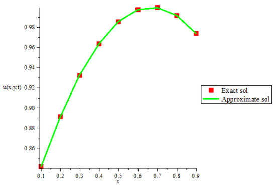
The proposed fourth-order new implicit difference scheme is applied to a 2D-TFMSDE. Table 1 compares the numerical results of the proposed scheme with the previous studies. In [17], the problem was solved using a compact difference scheme and, in [1], by a finite difference scheme. The scheme proposed in this paper shows better accuracy as the space and time steps are reduced. The order of the proposed method is $O({(\Delta x)}^4+{(\Delta y)}^4)$ in space variables and $O\left(\tau \right)$ in time variable [37]. The computational $C_1$-order and $C_2$-order are close to theoretical order, as can be seen in Table 1 and Table 2, respectively. For more confirmation, the proposed method is also extended to 2D RSP-HGSGF and the numerical results compared with the exact solution. The obtained results in Table 3 show very good accuracy for different values of $\gamma$, space, and time steps for Example 2. The 3D plots in Figure 1 and Figure 2 show the comparison of approximate and exact solution, and the 2D plot in Figure 3 shows the difference between the approximate and exact solution at $\alpha =0.25$, $\beta =0.45$, $T=1$, $M_x=M_y=10$, and $N=160$ for Example 1 with good agreement and high accuracy.

Table 1. Comparison of fourth-order implicit difference scheme for Equation (35), the error $E_{\infty }$ at $T=1.0,$ $\Delta x=\Delta y=\frac{1}{10}$, $\alpha =0.25,\beta =0.45$.

$\mathit{\tau }$	[17]	[1]	Scheme	${\mathit{C}}_1$-Order of Scheme
$1/10$	1.5729 × 10${}^{-2}$	5.1782 × 10${}^{-3}$	4.9806 × 10${}^{-3}$	-
$1/20$	7.8976 × 10${}^{-3}$	2.4390 × 10${}^{-3}$	2.2450 × 10${}^{-3}$	1.1497
$1/40$	3.9560 × 10${}^{-3}$	1.1772 × 10${}^{-3}$	9.8504 × 10${}^{-4}$	1.1885
$1/80$	1.9794 × 10${}^{-3}$	5.9755 × 10${}^{-4}$	4.0617 × 10${}^{-4}$	1.2782
$1/160$	9.8995 × 10${}^{-4}$	3.3033 × 10${}^{-4}$	1.3919 × 10${}^{-4}$	1.5451

Table 2. The order of convergence of fourth-order implicit difference scheme for Equation (35), the error $E_{\infty }$ at $T=1.0$, $\alpha =0.2,\beta =0.8$.

		Scheme	${\mathit{C}}_2$-Order
$\tau =h_x=h_y=1/4$		1.6406 × 10${}^{-2}$	-
$\tau =1/8,h_x=h_y=1/64$		7.3344 × 10${}^{-4}$	4.4838
$\tau =h_x=h_y=1/8$		8.2233 × 10${}^{-3}$	-
$\tau =1/16,h_x=h_y=1/128$		3.8694 × 10${}^{-4}$	4.4099

Table 3. Comparison of fourth-order implicit difference scheme for Equation (39) with the exact solution (43), the error $E_{\infty }$ at $T=1.0,$ $\Delta x=\Delta y=\frac{1}{10}$, $\alpha =0.25,\beta =0.45$.

$\mathit{\gamma }$	${(\mathbf{\Delta }\mathit{x})}^2={(\mathbf{\Delta }\mathit{y})}^2=\mathit{\tau }=1/16$	${(\mathbf{\Delta }\mathit{x})}^2={(\mathbf{\Delta }\mathit{y})}^2=\mathit{\tau }=1/64$	${(\mathbf{\Delta }\mathit{x})}^2={(\mathbf{\Delta }\mathit{y})}^2=\mathit{\tau }=1/144$
$0.5$	5.0794 × 10${}^{-3}$	1.4043 × 10${}^{-3}$	6.2458 × 10${}^{-4}$
$0.6$	5.9521 × 10${}^{-3}$	1.6387 × 10${}^{-3}$	6.8873 × 10${}^{-4}$
$0.7$	6.7049 × 10${}^{-3}$	1.8575 × 10${}^{-3}$	7.5239 × 10${}^{-4}$
$0.8$	7.4635 × 10${}^{-3}$	2.1414 × 10${}^{-3}$	8.1996 × 10${}^{-4}$
$0.9$	8.2610 × 10${}^{-3}$	2.3888 × 10${}^{-3}$	8.9478 × 10${}^{-4}$

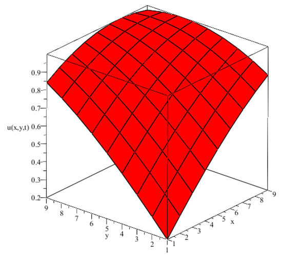
Figure 1. Exact solution.

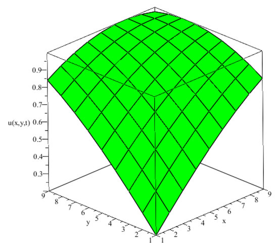
Figure 2. Approximate solution.

Figure 3. Comparison of the compact difference scheme in Equation (35) and the exact solution in Equation (38) at $\alpha =0.25,$ $\beta =0.45$, $T=1,y=0.1$, and $N=160$.

For a wide range of $\tau$, the results remain stable, indicating that the developed scheme is unconditionally stable (as shown in the theoretical analysis).

Example 2.

The following 2D Rayleigh–Stokes problem for heated generalized second-grade fluid (RSP-HGSGF) [22] is considered

$$\begin{array}{c}\hfill \frac{\partial u(x,y,t)}{\partial t}\hspace{1em}=\hspace{1em}\frac{{\partial }^{1-\gamma }}{\partial t^{1-\gamma }}\left(\frac{{\partial }^{2}u(x,y,t)}{\partial x^2}+\frac{{\partial }^{2}u(x,y,t)}{\partial y^2}\right)+\frac{{\partial }^{2}u(x,y,t)}{\partial x^2}+\frac{{\partial }^{2}u(x,y,t)}{\partial y^2}+f(x,y,t),\end{array}$$

(39)

where

$$f(x,y,t)=\left((1+\gamma )t^{1+\gamma }-\frac{2\Gamma (2+\gamma )}{\Gamma (1+2\gamma )}{t}^{2\gamma }-2t^{1+2\gamma }\right)e^{x+y},$$

(40)

subject to the initial condition

$$u(x,y,0)=0,0\le x,y\le 1,$$

(41)

$$\begin{array}{l}u(0,y,t)=e^y{t}^{1+\gamma },u(1,y,t)=e^{1+y}{t}^{1+\gamma },\\ \hspace{1em}\hspace{1em}\hspace{1em}\hspace{1em}\hspace{1em}\hspace{1em}\hspace{1em}\hspace{1em}\hspace{1em}\hspace{1em}\hspace{1em}u(x,0,t)=e^x{t}^{1+\gamma },u(x,1,t)=e^{1+x}{t}^{1+\gamma },\\ \hspace{1em}\hspace{1em}\hspace{1em}\hspace{1em}\hspace{1em}\hspace{1em}\hspace{1em}\hspace{1em}\hspace{1em}\hspace{1em}\hspace{1em}\hspace{1em}\hspace{1em}\hspace{1em}\hspace{1em}\hspace{1em}\hspace{1em}\hspace{1em}\hspace{1em}\hspace{1em}\hspace{1em}\hspace{1em}\hspace{1em}\hspace{1em}\hspace{1em}\hspace{1em} 0\le x,y\le 1,0\le t\le T.\end{array}$$

(42)

The exact solution is

$$u(x,y,t)=e^{x+y}{t}^{1+\gamma }.$$

(43)

4. Conclusions

In this paper, a fourth-order implicit difference scheme for time-fractional modified sub-diffusion equation is developed, analyzed, and applied. The von Neumann analysis is used to show the scheme is unconditionally stable. The results of an application to a particular examples are discussed. The numerical results seem to confirm the theoretical results and indicate the effectiveness and feasibility of the new formulated scheme. The numerical method in this paper can be applied to other types of fractional differential equations and higher-dimensional problems.

References

- Ali, U.; Abdullah, F.A.; Mohyud-Din, S.T. Modified implicit fractional difference scheme for 2D modified anomalous fractional sub-diffusion equation. Adv. Diff. Equ. 2017, 1–14. [Google Scholar] [CrossRef]
- Liu, F.; Yang, C.; Burrage, K. Numerical method and analytical technique of the modified anomalous subdiffusion equation with a nonlinear source term. J. Comput. Appl. Math. 2009, 231, 160–176. [Google Scholar] [CrossRef]
- Langlands, T.A.M. Solution of a modified fractional diffusion equation. Physica A 2006, 367, 136–144. [Google Scholar] [CrossRef]
- Jiang, W.; Chen, Z. A collocation method based on reproducing kernel for a modified anomalous subdiffusion equation. Numer. Meth. Part. Differ. Equ. 2014, 30, 289–300. [Google Scholar] [CrossRef]
- Miller, K.S.; Ross, B. An Introductional the Fractional Calculus and Fractional Differential Equations; Academic Press: New York, NY, USA; London, UK, 1974. [Google Scholar]
- Oldham, K.B.; Spanier, J. The Fractional Calculus; Academic Press: New York, NY, USA; London, UK, 1974. [Google Scholar]
- Liangliang, M.A.; Dongbing, L. An implicit difference approximation for fractional cable equation in high-dimensional case. J. Liao. Tech. Univ. 2014, 4, 24. [Google Scholar]
- Zhuang, P.; Liu, F.; Anh, V.; Turne, I. New solution and analytical techniques of the implicit numerical methods for the anomalous sub-diffusion equation. SIAM J. Numer. Anal. 2008, 46, 1079–1095. [Google Scholar] [CrossRef]
- Li, Y.; Wang, D. Improved efficient difference method for the modified anomalous sub-diffusion equation with a nonlinear source term. Int. J. Comput. Math. 2016, 94, 821–840. [Google Scholar] [CrossRef]
- Dehghan, M.; Abbaszadeh, M.; Mohebbi, A. Legendre spectral element method for solving time fractional modified anomalous sub-diffusion equation. Appl. Math. Model 2015, 40, 3635–3654. [Google Scholar] [CrossRef]
- Cao, X.; Xianxian, C.; Wen, L. The implicit midpoint method for the modified anomalous sub-diffusion equation with a nonlinear source term. J. Comput. Appl. Math. 2016, 1–12. [Google Scholar] [CrossRef]
- Ding, H.; Li, C. High-order compact difference schemes for the modified anomalous subdiffusion equation. Numer. Meth. Part. Differ. Equ. 2015, 213–242. [Google Scholar] [CrossRef]
- Wang, Z.; Vong, S. Compact difference schemes for the modified anomalous fractional sub-diffusion equation and the fractional diffusion-wave equation. J. Comput. Phys. 2014, 277, 1–15. [Google Scholar] [CrossRef]
- Al-Shibani, F.S.; Ismail, A.I.M. Compact Crank-Nicolson and Du Fort-Frankel method for the solution of the anomalous time fractional diffusion equation. Int. J. Comput. Methods 2013, 12, 1550041. [Google Scholar] [CrossRef]
- Adell, J.A.; Lekuona, A. Note on two extensions of the classical formula for sums of powers on arithmetic progressions. Adv. Differ. Equ. 2017, 1–5. [Google Scholar] [CrossRef]
- Ali, U.; Abdullah, F.A.; Ismail, A.I. Crank-Nicolson finite difference method for two-dimensional fractional sub-diffusion equation. J. Interpolat. Approx. Sci. Comput. 2017, 2, 18–29. [Google Scholar] [CrossRef]
- Abbaszadeh, M.; Mohebbi, A. A fourth-order compact solution of the two-dimensional modified anomalous fractional sub-diffusion equation with a nonlinear source term. Comput. Math. Appl. 2013, 66, 1345–1359. [Google Scholar] [CrossRef]
- Mohebbi, A.; Abbaszadeh, M.; Dehghan, M. A high-order and unconditionally stable scheme for the modified anomalous fractional sub-diffusion equation with a nonlinear source term. J. Comput. Phys. 2013, 240, 36–48. [Google Scholar] [CrossRef]
- Gao, W.; Yel, G.; Baskonus, H.M.; Cattani, C. Complex solitons in the conformable (2+ 1)-dimensional Ablowitz-Kaup-Newell-Segur equation. AIMS Math. 2019, 5, 507–521. [Google Scholar] [CrossRef]
- Gao, W.; Veeresha, P.; Prakasha, D.G.; Baskonus, H.M.; Yel, G. A powerful approach for fractional Drinfeld–Sokolov–Wilson equation with Mittag-Leffler law. Alex. Eng. J. 2019, 58, 1301–1311. [Google Scholar] [CrossRef]
- Gao, W.; Ghanbari, B.; Baskonus, H.M. New numerical simulations for some real world problems with Atangana–Baleanu fractional derivative. Chaos Solitons Fract. 2019, 128, 34–43. [Google Scholar] [CrossRef]
- Chen, C.M.; Liu, F.; Anh, V. Numerical analysis of the Rayleigh–Stokes problem for a heated generalized second grade fluid with fractional derivatives. Appl. Math. Comput. 2008, 204, 340–351. [Google Scholar] [CrossRef]
- Ali, U.; Abdullah, F.A. Modified implicit difference method for one-dimensional fractional wave equation. In Proceedings of the AIP Conference Proceedings, Penang, Malaysia, 10–12 December 2018; Volume 2184, p. 060021. [Google Scholar]
- Sokolov, I.M.; Klafter, J. From diffusion to anomalous diffusion: A century after Einstein’s Brownian motion. Chaos 2005, 15, 026103. [Google Scholar] [CrossRef] [PubMed]
- Zhuang, P.; Liu, F.; Turner, L.; Anh, V. Galerkin finite element method and error analysis for the fractional cable equation. Numer. Algorithms 2016, 72, 447–466. [Google Scholar] [CrossRef]
- Oldham, K.B.; Spanier, J. The Fractional Calculus: Theory and Application of Differentiation and Integration to Arbitrary Order; Academic Press: Cambridge, MA, USA, 1974. [Google Scholar]
- Metzler, R.; Klafter, J. The restaurant at the end of the random walk: Recent developments in the description of anomalous transport by fractional dynamics. J. Phys. A 2004, 37, R161–R208. [Google Scholar] [CrossRef]
- Hu, Z.; Zhang, L. Implicit compact difference schemes the fractional cable equation. Appl. Math. Model 2012, 36, 4027–4043. [Google Scholar] [CrossRef]
- Gang, G.; Kun, L.; Yuhui, W. Exact solutions of a modified fractional diffusion equation in the finite and semi-infinite domains. Physica A 2015, 417, 193–201. [Google Scholar]
- Jumarie, G. Modified Riemann-Liouville derivative and fractional Taylor series of non-differentiable functions further results. Comput. Math. Appl. 2006, 51, 1367–1376. [Google Scholar]
- Podulbny, I. Fractional Differential Equations; Academic Press: New York, NY, USA, 1999. [Google Scholar]
- Ali, U.; Abdullah, F.A. Explicit Saul’yev finite difference approximation for two-dimensional fractional sub-diffusion equation. In Proceedings of the AIP Conference Proceedings, Pahang, Malaysia, 27–29 August 2018; Volume 1, p. 020111. [Google Scholar]
- Liu, F.; Yang, Q.; Turner, I. Two new implicit numerical methods for the fractional cable equation. J. Comput. Nonlinear Dyn. 2011, 6, 1–7. [Google Scholar] [CrossRef]
- Chen, C.M.; Liu, F.; Turner, I.; Anh, V. Numerical methods with fourth-order spatial accuracy for variable-order nonlinear Stocks’ first problem for a heated generalized second grade fluid. Comput. Math. Appl. 2011, 62, 971–986. [Google Scholar] [CrossRef]
- Liu, Q.; Liu, F.; Turner, I.; Anh, V. Finite element approximation for a modified anomalous subdiffusion equation. Appl. Math. Model 2011, 35, 4103–4116. [Google Scholar] [CrossRef]
- Oliveira, E.C.; Machado, J.A.T. A Review of Definitions for Fractional Derivatives and Integral. Math. Probl. Eng. 2014, 2014, 238459. [Google Scholar] [CrossRef]
- Ali, U. Numerical Solutions for two Dimensional Time-Fractional Differential Sub-Diffusion Equation. Ph.D. Thesis, University Sains Malaysia, Penang, Malaysia, 2019; pp. 1–200. [Google Scholar]
© 2020 by the authors. Licensee MDPI, Basel, Switzerland. This article is an open access article distributed under the terms and conditions of the Creative Commons Attribution (CC BY) license (http://creativecommons.org/licenses/by/4.0/).