On the Metric Dimension of Arithmetic Graph of a Composite Number

Abstract

This paper is devoted to the study of the arithmetic graph of a composite number m, denoted by ${\mathcal{A}}_m$. It has been observed that there exist different composite numbers for which the arithmetic graphs are isomorphic. It is proved that the maximum distance between any two vertices of ${\mathcal{A}}_m$ is two or three. Conditions under which the vertices have the same degrees and neighborhoods have also been identified. Symmetric behavior of the vertices lead to the study of the metric dimension of ${\mathcal{A}}_m$ which gives minimum cardinality of vertices to distinguish all vertices in the graph. We give exact formulae for the metric dimension of ${\mathcal{A}}_m$, when m has exactly two distinct prime divisors. Moreover, we give bounds on the metric dimension of ${\mathcal{A}}_m$, when m has at least three distinct prime divisors.

1. Introduction

All graphs considered in this paper are simple, undirected, connected and finite. A graph G consists of two sets, $V\left(G\right)$ and $E\left(G\right)$, known as the vertex set and the edge set of G, respectively. The elements of $V\left(G\right)$ and $E\left(G\right)$ are called the vertices and edges of G, respectively. An element e of $E\left(G\right)$ is an unordered pair of two elements say $x,y$ of $V\left(G\right)$ and the two vertices x and y forming edge e are called adjacent vertices and written as $x\sim y$. The set $\{x\in V(G\left)\right|x\sim y\}$ is called the open neighborhood of y in G, denoted as $N_G\left(y\right)$. The set $N_G\left(y\right)\cup \{y\}$ is called the closed neighborhood of y in G, denoted as $N_G\left[y\right]$. $N_G\left(y\right)$ and $N_G\left[y\right]$ will be denoted by $N\left(y\right)$ and $N\left[y\right]$ respectively if G is clear from the context. Please note that the $distance$ between the two vertices u and v of a graph G, denoted by $d_G(u,v)$ and $d(u,v)$ if G is clear from the context, is the minimum number of edges traversed from u to v in G. For basic concepts of graph theory, please see [1].

The concept of resolving set and the metric dimension of a graph was introduced by Slater [2] as well as by Harary and Melter [3] independently. Slater used this concept for uniquely identifying the location of a vertex in the graph. Applications of this concept exists in coin-weighing problems [4,5], Master mind game [6], digital images [7], chemistry [8], isomorphism problem [9], network discovery and verification [10]. Moreover, Bailey and Cameron used this concept and obtained bounds on the possible orders of primitive permutation groups [11] (see also [12]).

A subset R of the vertices of a graph G satisfying the property that for every two distinct vertices $x,y\in V\left(G\right)$ there exist $r\in R$ such that $d(x,r)\ne d(y,r)$ is called a $resolving$ $set$ for G and $dim\left(G\right)$ denotes the minimum cardinality of a resolving set for G which we called the $metric$ $dimension$ of G. Due to the fact that finding the metric dimension of a graph is NP-complete [13,14] and it has applications in different fields, many researchers put their attention towards computing this parameter for known classes of graphs. For example, this parameter is studied in Cayley digraphs [15], wheels [16], unicyclic graphs [17], Cartesian products [18] and trees [2,3]. Moreover, Imran et al. studied the metric dimension of gear graphs [19] and symmetric graphs obtained by rooted product [20], Hussain et al. [21] studied the metric dimension of 2D lattice of alpha-boron nanotubes, Bailey et al. [11] studied the metric dimension of Johnson and Kneser graphs, Ahmad et al. [22] studied the metric dimension of generalized Petersen graphs, Min Feng et al. [23] studied the metric dimension of the power graph of a finite group. Recently, Gerold and Frank [24] studied the metric dimension of ${\mathbb{Z}}_n\times {\mathbb{Z}}_n\times {\mathbb{Z}}_n$ and proved that $dim({\mathbb{Z}}_n\times {\mathbb{Z}}_n\times {\mathbb{Z}}_n)=\lfloor \frac{3n}{2}\rfloor$ where ${\mathbb{Z}}_n$ is the set of modulo classes of a natural number $n\ge 2$. Here in this article, we study the metric dimension of an arithmetic graph associated with a composite number.

Connections between number theory and graph theory have been studied by many authors, for examples see [25,26,27,28]. We observe that different numbers exhibit similar characteristics in connection with graphs. The graph associated with a given composite number form equivalence classes, for example, vertices can be partitioned based on twin classes. Distinguishing vertices of graphs using distances has been an interesting problem and gives useful insights about the structure of the graphs. Hence metric dimension of an arithmetic graph is being studied to grasp properties of the arithmetic graph. Throughout this paper, m is a composite number with the prime decomposition $m=p_1^{{\gamma }_1}{p}_2^{{\gamma }_2}{p}_3^{{\gamma }_3}$…$p_t^{{\gamma }_t}$, where $t\ge 2$, $p_i^{\prime }s$ are distinct primes and ${\gamma }_i\ge 1$ for each $1\le i\le t$. Every positive divisor $x\ne 1$ of m has the form $x=p_1^{{\alpha }_1}{p}_2^{{\alpha }_2}{p}_3^{{\alpha }_3}\dots p_t^{{\alpha }_t}$, where $0\le {\alpha }_i\le {\gamma }_i$ for each i and at least one ${\alpha }_i\ne 0$ for some i. If ${\alpha }_i\ne 0$ for some i, then $p_i$ is called a $primary$ $factor$ of x and the factor $p_i^{{\alpha }_i}$ is called a $secondary$ $factor$ of x if ${\alpha }_i\ge 2$. Two distinct divisors $x,y$ of m are said to have same $parity$ if they have same primary factors (i.e., $x=p_1{p}_2$ and $y=p_1^2{p}_2^3$ have same parity). An arithmetic graph ${\mathcal{A}}_m$ of a composite number m has the vertex set $V_m$ which contains all possible divisors $x\ne 1$ of m. Further two distinct vertices $x,y\in V_m$ are adjacent if and only if they have different parity and $gcd(x,y)=p_i$ (greatest common divisor) for some $i\in \{1,2,\dots ,t\}$. In [29,30], the authors studied the domination parameters of an arithmetic graphs. In [31], Suryanarayana and Sreenivansan studied the split domination in arithmetic graphs. Moreover, Vasumathi and Vangipuram [32] studied annihilator domination in arithmetic graphs.

In the next section, we study the diameter of ${\mathcal{A}}_m$ and prove that it is either 2 or 3, for any choice of composite number m. We study the properties of false twin vertices in arithmetic graphs. We study the metric dimension of ${\mathcal{A}}_m$ and give formulae for $dim\left({\mathcal{A}}_m\right)$ when m has exactly two primary factors. Moreover, we give bounds on the metric dimension of ${\mathcal{A}}_m$ when m has at least three primary factors. We also prove that there exist different composite numbers for which the arithmetic graphs are isomorphic.

2. Results

Please note that for every $m=p_1^{{\gamma }_1}{p}_2^{{\gamma }_2}{p}_3^{{\gamma }_3}$…$p_t^{{\gamma }_t}$, where $t\ge 2$, $p_i^{\prime }s$ are distinct primes and ${\gamma }_i\ge 1$ for each $1\le i\le t$, the arithmetic graph ${\mathcal{A}}_m$ is connected. In the next proposition, we give formula for the order of ${\mathcal{A}}_m$.

Proposition 1.

For every composite number m, we have $|V_m|={\displaystyle \prod _{i=1}^t}({\gamma }_i+1)-1$.

The $degree$ of a vertex p in a graph G is the cardinality of its open neighborhood, denoted as $de{g}_G\left(p\right)$ (simply $deg\left(p\right)$). The next proposition follows directly from the definition of ${\mathcal{A}}_m$.

Proposition 2.

For every primary factor $p_i$ of m, the degree of the vertex $p_i$ is given as $deg\left(p_i\right)={\gamma }_i\left|V_{m^{\prime }}\right|$, where $m^{\prime }={\gamma }_1{\gamma }_2\dots {\gamma }_{i-1}{\gamma }_{i+1}\dots {\gamma }_t$.

Please note that for every composite number m, the arithmetic graph ${\mathcal{A}}_m$ is connected. Let $P_i$ denote the set of all vertices of ${\mathcal{A}}_m$ with exactly i primary factors then the collection $P_1,P_2,\dots ,P_t$ gives a partition of $V_m$. The $diameter$ of a graph G, denoted by $diam\left(G\right)$, is the maximum distance between any pair of vertices of G. In the next theorem, we characterize the arithmetic graphs ${\mathcal{A}}_m$ with respect to diameter.

Theorem 1.

For every composite number $m=p_1^{{\gamma }_1}{p}_2^{{\gamma }_2}\dots p_t^{{\gamma }_t}$, the following assertions hold:

(i) 

$diam\left({\mathcal{A}}_m\right)=2$ if and only if ${\displaystyle {\displaystyle \sum }_{i=1}^t}{\gamma }_i=t$.

(ii) 

$diam\left({\mathcal{A}}_m\right)=3$ if and only if ${\displaystyle {\displaystyle \sum }_{i=1}^t}{\gamma }_i\ge t+1$.

Proof. 

(i) For ${\displaystyle {\displaystyle \sum }_{i=1}^t}{\gamma }_i=t$, no two distinct vertices of ${\mathcal{A}}_m$ have same parity. For any two non-adjacent vertices $x,y\in V_m$, we have the following cases:

Case 1. Suppose x and y have no common primary factor, then for any primary factor $p_i$ of x and $p_j$ of y, $p_i{p}_j\in N\left(x\right)\cap N\left(y\right)$ so $d(x,y)=2$.

Case 2. Suppose $p_i$ be a common primary factor of x and y, then $p_i\in N\left(x\right)\cap N\left(y\right)$. Hence, $diam\left({\mathcal{A}}_m\right)=2$.

Conversely, suppose $d\left({\mathcal{A}}_m\right)=2$, we are to show that ${\displaystyle {\displaystyle \sum }_{i=1}^t}{\gamma }_i=t$. Assume contrary that ${\displaystyle {\displaystyle \sum }_{i=1}^t}{\gamma }_i>t$, then there exist at least one primary factor $p_i$ such that ${\gamma }_i\ge 2$ and $d(x,y)=3$ when $x=p_1{p}_2\dots p_i^2{p}_{i+1}\dots p_t$ and $y=p_i^2$, a contradiction. Hence, ${\displaystyle {\displaystyle \sum }_{i=1}^t}{\gamma }_i=t$.

(ii) Suppose $diam\left({\mathcal{A}}_m\right)=3$, then by part (i), ${\displaystyle {\displaystyle \sum }_{i=1}^t}{\gamma }_i>t$.

Conversely, suppose ${\displaystyle {\displaystyle \sum }_{i=1}^t}{\gamma }_i>t$, we are to show that $diam\left({\mathcal{A}}_m\right)=3$. For any two non-adjacent distinct vertices $x,y\in V_m$, we have the following cases:

Case 1. Suppose $x,y\in P_1$ and $x,y$ have distinct parity then $p_i{p}_j\in N\left(x\right)\cap N\left(y\right)$, where $p_i$ is a primary factor of x and $p_j$ is a primary factor of y. Also, if $x,y$ have same parity then for any $p_j$, $j\ne i$, $p_i{p}_j\in N\left(x\right)\cap N\left(y\right)$. Hence, $d(x,y)=2$.

Case 2. Suppose $x\in P_1$, $y\in P_t$ be two non-adjacent vertices. Since no two vertices of $P_1$ are adjacent, further suppose no two vertices of $P_t$ are adjacent and y is not adjacent to any $z\in V_m\backslash (P_1\cup P_t)$. Hence, $d(x,y)=3$.

Case 3. For $x\in P_1$ and $y\in P_j$; $2\le j\le t-1$, we have $d(x,y)=2$.

Case 4. Suppose $x\in P_i$ and $y\in P_j$; $2\le i,j\le t$ be two distinct vertices. Suppose x and y have a primary common factor say $p_i$, then $d(x,y)=2$ because $pi\in N\left(x\right)\cap N\left(y\right)$. If $x,y$ have no common primary factor then $p_i{p}_j\in N\left(x\right)\cap N\left(y\right)$, where $p_i$ is a primary factor of x and $p_j$ is a primary factor of y.

By concluding the above four cases, we have $diam\left({\mathcal{A}}_m\right)=3$. □

In the next proposition, we describe the conditions on the exponents of the primary factors of m under which they have same degrees.

Proposition 3.

For any two distinct primary factors $p_i$ and $p_j$ of a composite number m, $deg\left(p_i\right)=deg\left(p_j\right)$ in ${\mathcal{A}}_m$ if and only if ${\gamma }_i={\gamma }_j$.

Proof. 

Suppose $deg\left(p_i\right)=deg\left(p_j\right)$, we are to show that ${\gamma }_i={\gamma }_j$. Assume contrary that ${\gamma }_i\ne {\gamma }_j$ and ${\gamma }_i<{\gamma }_j$, then $|N\left(p_i\right)\cap P_k|<|N\left(p_j\right)\cap P_k|$ for $2\le k\le t-1$. Since, $N\left(p_i\right)\cap P_1=N\left(p_j\right)\cap P_1=\varnothing$ and $N\left(p_i\right)\cap P_t=N\left(p_j\right)\cap P_t=P_t$ so $deg\left(p_i\right)<deg\left(p_j\right)$ because $P_1,P_2,\dots ,P_t$ gives a partition of $V_m$, a contradiction. Hence, ${\gamma }_i={\gamma }_j$.

Conversely, suppose that ${\gamma }_i={\gamma }_j$ for any two distinct primary factors $p_i,p_j$ of m, then $|N\left(p_i\right)\cap P_k|=|N\left(p_j\right)\cap P_k|$ for $1\le k\le t$. Hence, $deg\left(p_i\right)=deg\left(p_j\right)$. □

Two distinct vertices u and v are called $true$ $twins$ ($false$ $twins$) if $N\left[u\right]=N\left[v\right]$ ($N\left(u\right)=N\left(v\right)$). Two vertices are called $twins$ if they are either true twins or false twins. For any composite number $m=p_1^{{\gamma }_1}{p}_2^{{\gamma }_2}\dots p_t^{{\gamma }_t}$ such that ${\gamma }_i\le 2$ for each i and $t\ge 3$, ${\mathcal{A}}_m$ has no twins. Furthermore, no two adjacent vertices of ${\mathcal{A}}_m$ are twins. In next lemma, we prove that any two twin vertices in ${\mathcal{A}}_m$ have same parity which gives that both belong to $P_i$ for some i.

Lemma 1.

Any two distinct vertices $x,y$ in an arithmetic graph ${\mathcal{A}}_m$ of a composite number $m=p_1^{{\gamma }_1}{p}_2^{{\gamma }_2}\dots p_t^{{\gamma }_t}$; $t\ge 3$ are twins if and only if they have same parity and for any prime factor $p_i$ of x and y such that α is exponent of $p_i$ in x and β is exponent of $p_i$ in y, if ${\gamma }_i=2$, then $\alpha =\beta$ and if ${\gamma }_i\ge 3$ with $\alpha \ne \beta$, then $\alpha ,\beta \ge 2$.

Proof. 

Suppose $x,y$ are twins in ${\mathcal{A}}_m$ and have distinct parity. If $p_i$ is a factor of x and $p_i$ is not a factor of y, then $N\left(x\right)\ne N\left(y\right)$ which directly follows from the definition of the arithmetic graph. Hence, $x,y$ have same parity. Now suppose $p_i$ is a factor of x and y such that ${\gamma }_i=2$ and $\alpha =1$, we are to show that $\beta =1$. Assume contrary that $\beta \ge 2$, then $N\left(x\right)\ne N\left(y\right)$. Next suppose that ${\gamma }_i\ge 3$ and $\alpha \ne \beta$, we are to show that $\alpha ,\beta \ge 2$. Assume contrary that $\alpha =1$, then by the definition of the arithmetic graph $x,y$ are not twins, a contradiction. Hence, $\alpha ,\beta \ge 2$.

The converse follows directly from the definition of the arithmetic graph, when x and y have same parity and for any prime factor $p_i$ of x and y such that $\alpha$ is exponent of $p_i$ in x and $\beta$ is exponent of $p_i$ in y, if ${\gamma }_i=2$, then $\alpha =\beta$ and if ${\gamma }_i\ge 3$ with $\alpha \ne \beta$, then $\alpha ,\beta \ge 2$. □

Metric Dimension of Arithmetic Graphs

The following result helps in finding resolving sets and the metric dimension of a graph containing twins.

Corollary 1.

([33]). Suppose R is a resolving set for a connected graph G and $a,b\in V\left(G\right)$ are twins. Then a or b is in R. Moreover, if $a\in R$ and $b\notin R$, then $(R\backslash \{a\})\cup \{b\}$ is also a resolving set for G.

For a composite number m with the canonical form $m=p_1{p}_2$, the arithmetic graph ${\mathcal{A}}_m$ is isomorphic to a path graph on three vertices and has metric dimension 1. In the next result, we find the metric dimension of ${\mathcal{A}}_m$ when m has exactly two distinct primary factors.

Theorem 2.

For every composite number m with the canonical form $m=p_1^{{\gamma }_1}{p}_2^{{\gamma }_2}$, where $1\le {\gamma }_1,{\gamma }_2$ and ${\gamma }_1+{\gamma }_2\ge 3$, we have

(i) 

For ${\gamma }_1=1$ and ${\gamma }_2=2$, $dim\left({\mathcal{A}}_m\right)=2$.

(ii) 

For ${\gamma }_1=1$ and ${\gamma }_2\ge 3$, $dim\left({\mathcal{A}}_m\right)=2{\gamma }_2-3$.

(iii) 

For ${\gamma }_1=2$ and ${\gamma }_2=2$, $dim\left({\mathcal{A}}_m\right)=3$.

(iv) 

For ${\gamma }_1=2$ and ${\gamma }_2\ge 3$, $dim\left({\mathcal{A}}_m\right)=2+3({\gamma }_2-2)$.

(v) 

For ${\gamma }_1,{\gamma }_2\ge 3$, $dim\left({\mathcal{A}}_m\right)=1+2({\gamma }_1-2)+2({\gamma }_2-2)+(({\gamma }_1-1)({\gamma }_2-1)-1)$.

Proof. 

Using the definition of the arithmetic graph, we have $N\left(p_1\right)=N\left(p_2\right)$. As, ${\mathcal{A}}_m$ for $m=p_1^{{\gamma }_1}{p}_2^{{\gamma }_2}$ with ${\gamma }_1+{\gamma }_2\ge 3$ is not a path graph so $dim\left({\mathcal{A}}_m\right)\ge 2$.

(i) For ${\gamma }_1=1$ and ${\gamma }_2=2$, the set $W=\{p_1,p_2^2\}$ is a resolving set for ${\mathcal{A}}_m$. Hence, $dim\left({\mathcal{A}}_m\right)=2$.

(ii) For ${\gamma }_1=1$ and ${\gamma }_2\ge 3$, the classes $\{p_1,p_2\}$, $\{p_2^2,\dots ,p_2^{{\gamma }_2}\}$ and $\{p_1{p}_2^2,\dots ,p_1{p}_2^{{\gamma }_2}\}$ are equivalence classes of false twins in ${\mathcal{A}}_m$ and by using Corollary 1, we have $dim({\mathcal{A}}_m\ge 1+2({\gamma }_2-2)=2{\gamma }_2-3$. Consider $W=\{p_1,p_2^2,\dots$, $p_2^{{\gamma }_2-1},p_1{p}_2^2,$$\dots ,p_1{p}_2^{{\gamma }_2-1}\}$, we prove that W is a resolving set for ${\mathcal{A}}_m$. Let $x\ne y\in V_m\backslash W$ then we have following cases:

Case 1. Suppose $x,y\in P_1$ yields that $x=p_2$ and $y=p_2^{{\gamma }_2}$ and $p_1{p}_2^2\in W$ such that $d(x,p_1{p}_2^2)\ne d(y,p_1{p}_2^2)$.

Case 2. Suppose $x,y\in P_2$ yields that $x=p_1{p}_2$ and $y=p_1{p}_2^{{\gamma }_2}$ and there exist $w=p_2^2\in W$ such that $d(x,w)\ne d(y,w)$.

Case 3. Suppose $x\in P_1$ and $y\in P_2$ yields that $x\in \{p_2,p_2^{{\gamma }_2}\}$ and $y\in \{p_1{p}_2,p_1{p}_2^{{\gamma }_2}\}$ and there exist $w=p_1\in W$ such that $d(x,w)\ne d(y,w)$.

Concluding all above cases, W is a resolving set for ${\mathcal{A}}_m$. Hence, $dim\left({\mathcal{A}}_m\right)=1+2({\gamma }_2-2)=2{\gamma }_2-3$.

(iii) For ${\gamma }_1=2$ and ${\gamma }_2=2$, suppose that $dim\left({\mathcal{A}}_m\right)=2$, then any resolving set W will have the form $W=\{p_1,x\}$. Let $x\in P_1$ then W is not a resolving set for ${\mathcal{A}}_m$ because $p_1^2$ does not resolves $p_1{p}_2$ and $p_1{p}_2^2$ and $p_2^2$ does not resolves the pair $p_1{p}_2$ and $p_1^2{p}_2^2$. Furthermore, for any $x\in P_2$, W is not a resolving set for ${\mathcal{A}}_m$, hence $dim\left({\mathcal{A}}_m\right)\ge 3$. Now, the set $W=\{p_1,p_1^2,p_2^2\}$ is a resolving set for ${\mathcal{A}}_m$ so $dim\left({\mathcal{A}}_m\right)=3$.

(iv) For ${\gamma }_1=2$ and ${\gamma }_2\ge 3$, the classes $\{p_1,p_2\}$, $\{p_2^2,\dots ,p_2^{{\gamma }_2}\}$, $\{p_1{p}_2^2,\dots ,p_1{p}_2^{{\gamma }_2}\}$ and $\{p_1^2{p}_2^2,\dots ,p_1^2{p}_2^{{\gamma }_2}\}$ are equivalence classes of false twins in ${\mathcal{A}}_m$. Corollary 1 gives that $dim\left({\mathcal{A}}_m\right)\ge 1+3({\gamma }_2-2)$. Consider $W=\{p_1,p_2^2,$$\dots ,$$p_2^{{\gamma }_2-1},p_1{p}_2^2,\dots ,p_1{p}_2^{{\gamma }_2-1}{p}_1^2{p}_2^2,\dots ,p_1^2{p}_2^{{\gamma }_2-1}\}$ satisfying the conditions of Corollary 1 and note that for $x=p_1{p}_2$, $y=p_1^2{p}_2\in V_m\backslash W$ then $d(x,w)=d(y,w)$ for each $w\in W$ which gives that W is not a resolving set for ${\mathcal{A}}_m$. Hence, $dim\left({\mathcal{A}}_m\right)\ge 2+3({\gamma }_2-2)$. Now to prove that $dim\left({\mathcal{A}}_m\right)\le 2+3({\gamma }_2-2)$, we only need to prove that $W_1=\{p_1,p_1^2,p_2^2,$$\dots ,$$p_2^{{\gamma }_2-1},p_1{p}_2^2,\dots ,p_1{p}_2^{{\gamma }_2-1}{p}_1^2{p}_2^2,\dots ,p_1^2{p}_2^{{\gamma }_2-1}\}$ is a resolving set for ${\mathcal{A}}_m$. Let $x\ne y\in V_m\backslash W_1$, we study the following cases:

Case 1. Suppose $x,y\in P_1$ implies that $x=p_2$ and $y=p_2^{{\gamma }_2}$ and $w=p_1{p}_2\in W_1$ such that $d(x,w)\ne d(y,w)$.

Case 2. Suppose $x,y\in P_2$ then $x,y\in \{p_1{p}_2,p_1^2{p}_2,p_1{p}_2^{{\gamma }_2},p_1^2{p}_2^{{\gamma }_2}\}$. For $x=p_1{p}_2$ and $y\in \{p_1^2{p}_2,p_1^2{p}_2^{{\gamma }_2}\}$ there exist $w=p_1^2\in W_1$ such that $d(x,w)\ne d(y,w)$. For $x=p_1{p}_2$ and $y=p_1{p}_2^{{\gamma }_2}$ there exist $w=p_2^2\in W_1$ such that $d(x,w)\ne d(y,w)$. For $x=p_1^2{p}_2$ and $y=p_1{p}_2^{{\gamma }_2}$ there exist $w=p_1^2\in W_1$ such that $d(x,w)\ne d(y,w)$. For $x=p_1^2{p}_2$ and $y=p_1^2{p}_2^{{\gamma }_2}$ there exist $w=p_2^2\in W_1$ such that $d(x,w)\ne d(y,w)$. Now for $x=p_1{p}_2^{{\gamma }_2}$ and $y=p_1^2{p}_2^{{\gamma }_2}$ there exist $w=p_1^2\in W_1$ such that $d(x,w)\ne d(y,w)$.

Case 3. Suppose $x\in P_1$ and $y\in P_2$ implies that $x\in \{p_2,p_2^{{\gamma }_2}\}$ and $y\in \{p_1{p}_2,p_1^2{p}_2,p_1{p}_2^{{\gamma }_2},p_1^2{p}_2^{{\gamma }_2}\}$. For $x=p_2$ and $y\in \{p_1{p}_2,p_1^2{p}_2,p_1{p}_2^{{\gamma }_2},p_1^2{p}_2^{{\gamma }_2}\}$ there exist $w=p_1{p}_2^2\in W_1$ such that $d(x,w)\ne d(y,w)$. Now for $x=p_2^{{\gamma }_2}$ and $y\in \{p_1{p}_2,p_1^2{p}_2,p_1{p}_2^{{\gamma }_2},p_1^2{p}_2^{{\gamma }_2}\}$ there exist $w=p_1\in W_1$ such that $d(x,w)\ne d(y,w)$.

Concluding all above cases $W_1$ is a resolving set for ${\mathcal{A}}_m$.

(v) For ${\gamma }_1,{\gamma }_2\ge 3$, the sets $\{p_1,p_2\}$, $\{p_1^2,\dots ,p_1^{{\gamma }_1}\}$, $\{p_1^2{p}_2,\dots ,p_1^{{\gamma }_1}{p}_2\}$, $\{p_2^2,\dots ,p_2^{{\gamma }_2}\}$, $\{p_1{p}_2^2,\dots ,$$p_1{p}_2^{{\gamma }_2}\}$ and $\{p_1^2,\dots ,p_1^{{\gamma }_1}\}\times \{p_2^2,\dots ,p_2^{{\gamma }_2}\}$ are equivalence classes of false twins. Corollary 1 gives that $dim\left({\mathcal{A}}_m\right)\le 1+2({\gamma }_1-2)+2({\gamma }_2-2)+(({\gamma }_1-1)({\gamma }_2-1)-1)$. Now to prove that $dim\left({\mathcal{A}}_m\right)\ge 1+2({\gamma }_1-2)+2({\gamma }_2-2)+(({\gamma }_1-1)({\gamma }_2-1)-1)$ we only need to prove that $W=\{p_1,p_1^2,\dots ,p_1^{{\gamma }_1-1},p_2^2,\dots ,p_2^{{\gamma }_2-1},p_1^2{p}_2,\dots ,p_1^{{\gamma }_1-1}{p}_2,p_1{p}_2^2,\dots ,p_1{p}_2^{{\gamma }_2-1},p_1^2{p}_2^2,\dots ,p_1^{{\gamma }_1}{p}_2^{{\gamma }_2-1}\}$ is a resolving set for ${\mathcal{A}}_m$. Let $x\ne y\in V_m\backslash W$, we study the following cases:

Case 1. Suppose $x,y\in P_1$ implies that $x,y\in \{p_2,p_1^{{\gamma }_1},p_2^{{\gamma }_2}\}$. For $x=p_2$ and $y\in \{p_1^{{\gamma }_1},p_2^{{\gamma }_2}\}$ there exist $w=p_1^2{p}_2^2$ such that $d(x,w)\ne d(y,w)$. For $x=p_1^{{\gamma }_1}$ and $y=p_2^{{\gamma }_2}$ there exist $w=p_1{p}_2^2\in W$ such that $d(x,w)\ne d(y,w)$.

Case 2. Suppose $x,y\in P_2$ yields that $x,y\in \{p_1{p}_2,p_1{p}_2^{{\gamma }_2},p_1^{{\gamma }_1}{p}_2,p_1^{{\gamma }_1}{p}_2^{{\gamma }_2}\}$. For $x\in \{p_1{p}_2,p_1{p}_2^{{\gamma }_2}\}$ and $y\in \{p_1^{{\gamma }_1}{p}_2,p_1^{{\gamma }_1}{p}_2^{{\gamma }_2}\}$ there exist $w=p_1^2\in W$ such that $d(x,w)\ne d(y,w)$. For $x=p_1{p}_2$ and $y=p_1{p}_2^{{\gamma }_2}$ there exist $w=p_2^2\in W$ such that $d(x,w)\ne d(y,w)$.

Case 3. Suppose $x\in P_1$ and $y\in P_2$ yields that $x\in \{p_1^{{\gamma }_1},p_2,p_2^{{\gamma }_2}\}$ and $y\in \{p_1{p}_2,p_1{p}_2^{{\gamma }_2},p_1^{{\gamma }_1}{p}_2,p_1^{{\gamma }_1}{p}_2^{{\gamma }_2}\}$. Now for $x=p_1^{{\gamma }_1}$ and $y\in \{p_1^{{\gamma }_1}{p}_2,p_1{p}_2^{{\gamma }_2},p_1^{{\gamma }_1}{p}_2^{{\gamma }_2}\}$ there exist $w=p_2^2\in W$ such that $d(x,w)\ne d(y,w)$. For $x=p_1^{{\gamma }_1}$ and $y=p_1{p}_2$ there exist $w=p_1$ such that $d(x,w)\ne d(y,w)$. For $x=p_2$ and $y\in \{p_1{p}_2,p_1{p}_2^{{\gamma }_2},p_1^{{\gamma }_1}{p}_2,p_1^{{\gamma }_1}{p}_2^{{\gamma }_2}\}$ there exist $w=p_1$ such that $d(x,w)\ne d(y,w)$. Now for $x=p_2^{{\gamma }_2}$ and $y\in \{p_1{p}_2,p_1{p}_2^{{\gamma }_2},p_1^{{\gamma }_1}{p}_2,p_1^{{\gamma }_1}{p}_2^{{\gamma }_2}\}$ there exist $w=p_2^2$ such that $d(x,w)\ne d(y,w)$.

Concluding all above cases, W is a resolving set for ${\mathcal{A}}_m$. Hence, $dim\left({\mathcal{A}}_m\right)=1+2({\gamma }_1-2)+2({\gamma }_2-2)+(({\gamma }_1-1)({\gamma }_2-1)-1)$. □

The set of bold vertices represented by $p_1,p_2,p_3^2$ in Figure 1 forms a minimum resolving set for the arithmetic graph of $m=p_1{p}_2{p}_3^2$ shown in the figure and the set of bold vertices represented by $p_1,p_2,p_2^2,p_3^2$ in Figure 2 forms a minimum resolving set for the arithmetic graph of $m=p_1{p}_2^2{p}_3^2$ shown in the figure. Also, the set of bold vertices represented by $p_1,p_1^2,p_2,p_2^2,p_3^2$ in Figure 3 forms a minimum resolving set for the arithmetic graph of $m=p_1^2{p}_2^2{p}_3^2$ shown in the figure. Hence, we have the following lemma.

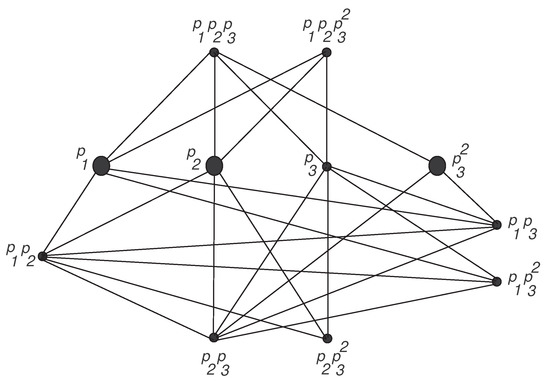
Figure 1. The arithmetic graph ${\mathcal{A}}_m$ of $m=p_1{p}_2{p}_3^2.$

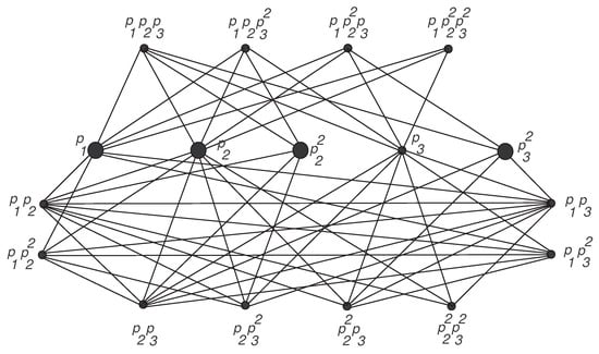
Figure 2. The arithmetic graph ${\mathcal{A}}_m$ of $m=p_1{p}_2^2{p}_3^2.$

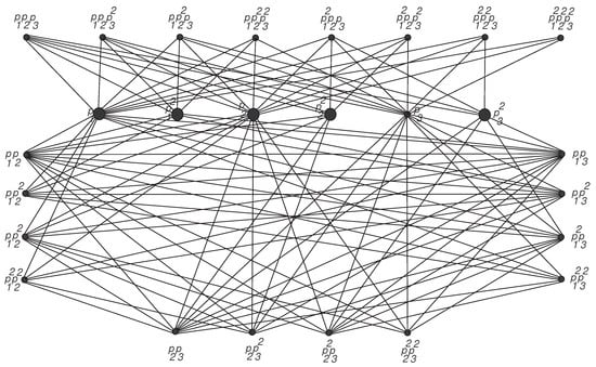
Figure 3. The arithmetic graph ${\mathcal{A}}_m$ of $m=p_1^2{p}_2^2{p}_3^2.$

Lemma 2.

For every composite number m with the canonical form $m=p_1^{{\gamma }_1}{p}_2^{{\gamma }_2}{p}_3^{{\gamma }_3}$ such that $1\le {\gamma }_i\le 2$ and at least one ${\gamma }_i=2$, we have $dim\left({\mathcal{A}}_m\right)={\displaystyle {\displaystyle \sum }_{i=1}^t}{\gamma }_i-1$.

In the next theorem, we give the formula for the metric dimension of ${\mathcal{A}}_m$ when m has at least four distinct primary factors.

Lemma 3.

For every positive integer m with the canonical form $m=p_1^{{\gamma }_1}{p}_2^{{\gamma }_2}\dots p_t^{{\gamma }_t}$ such that $1\le {\gamma }_i\le 2$ and $t\ge 4$, we have $dim\left({\mathcal{A}}_m\right)={\displaystyle {\displaystyle \sum }_{i=1}^t}{\gamma }_i$.

Proof. 

Consider $W=P_1\subset V_m$ such that $\left|W\right|={\displaystyle {\displaystyle \sum }_{i=1}^t}{\gamma }_i$. To show that W is a resolving set for ${\mathcal{A}}_m$, consider two distinct vertices $x,y\in V_m\backslash W$ then x and y have at least two primary factors. First suppose that x and y have same parity then there exists at least one $i\in \{1,2,\dots ,t\}$ such that $p_i$ is a factor of x and $p_i^2$ is a factor of y then $x,y$ are resolved by $p_i^2\in W$. Now suppose that x and y have different parity then there exists at least one $p_i$ for some i such that $p_i$ is a primary factor of x and $p_i$ is not a primary factor of y. Since, $p_i\in W$ so $x,y$ are resolved by W. Hence, W is a resolving set for ${\mathcal{A}}_m$ which gives that $dim\left({\mathcal{A}}_m\right)\le {\displaystyle \sum }{\gamma }_i$. Now to prove that $dim\left({\mathcal{A}}_m\right)\ge {\displaystyle \sum }{\gamma }_i$ assume contrary that $dim\left({\mathcal{A}}_m\right)<{\displaystyle \sum }{\gamma }_i$. Let $\acute{W}$ be a minimum resolving set for ${\mathcal{A}}_m$. Without loss of generality suppose that $|\acute{W}| ={\displaystyle \sum }{\gamma }_i-1$. We discuss the following two cases:

Case 1. Suppose $\acute{W}\subset P_1$ then there exists some $p_i$ or $p_j^2$ such that $p_i\notin \acute{W}$ or $p_j^2\notin \acute{W}$. First suppose that $p_i\notin \acute{W}$ and ${\gamma }_i=1$ then the vertices $u=p_1^{{\alpha }_1}{p}_2^{{\alpha }_2}\dots p_{i-1}^{{\alpha }_{i-1}}{p}_i{p}_{i+1}^{{\alpha }_{i+1}}\dots p_t^{{\alpha }_t}$ and $v=p_1^{{\alpha }_1}{p}_2^{{\alpha }_2}\dots p_{i-1}^{{\alpha }_{i-1}}{p}_{i+1}^{{\alpha }_{i+1}}\dots p_t^{{\alpha }_t}$ are not resolved by $\acute{W}$. Suppose $p_i\notin \acute{W}$ and ${\gamma }_i=2$ then the vertices $u=p_1^{{\alpha }_1}{p}_2^{{\alpha }_2}$$\dots p_{i-1}^{{\alpha }_{i-1}}{p}_i^2$$p_{i+1}^{{\alpha }_{i+1}}\dots p_t^{{\alpha }_t}$ and $v=p_1^{{\alpha }_1}{p}_2^{{\alpha }_2}\dots p_{i-1}^{{\alpha }_{i-1}}{p}_{i+1}^{{\alpha }_{i+1}}\dots p_t^{{\alpha }_t}$ are not resolved by $\acute{W}$. Hence, any proper subset of $P_1$ is not a resolving set for ${\mathcal{A}}_m$.

Case 2. Suppose $\acute{W}$ is not a subset of $P_1$ and $|\acute{W}\cap P_1| ={\displaystyle \sum }{\gamma }_i-2$. Let $\acute{w}\in \acute{W}\backslash P_1$ then there exists two distinct vertices $x,y\in P_1\backslash \acute{W}$. Since, $x,y$ are not resolved by any vertex in $\acute{W}\cap P_1$ so $x,y$ are resolved by $\acute{w}$. We have the following subcases:

Subcase 1. Suppose $x=p_i$ and $y=p_j$ for some $i\ne j$. Since, $\acute{w}$ resolves x and y so exactly one $p_i$ or $p_j$ is a primary factor of $\acute{w}$. Let $p_i$ is a factor of $\acute{w}$ and $p_j$ is not a primary factor of $\acute{w}$. Suppose ${\gamma }_j=1$ then the vertices $u=p_i$ and $v=p_i{p}_j$ are not resolved by $\acute{W}$. Now suppose that ${\gamma }_j=2$ then the vertices $u=p_i$ and $v=p_i{p}_j^2$ are not resolved by $\acute{W}$. Hence, $\acute{W}$ is not a resolving set for ${\mathcal{A}}_m$.

Subcase 2. Suppose $x=p_i$ and $y=p_i^2$ for some i. Since, $x,y$ are resolved by $\acute{w}$ so $p_i^2$ must be a secondary factor of $\acute{w}$. The vertices $u=p_1^{{\alpha }_1}{p}_2^{{\alpha }_2}\dots p_{i-1}^{{\alpha }_{i-1}}$$p_i^2$$p_{i+1}^{{\alpha }_{i+1}}\dots p_t^{{\alpha }_t}$ and $v=p_1^{{\alpha }_1}{p}_2^{{\alpha }_2}\dots p_{i-1}^{{\alpha }_{i-1}}{p}_i^2{p}_{i+1}^{{\alpha }_{i+1}}\dots p_t^{{\alpha }_t}$ are not resolved by $\acute{W}$ for at least one ${\alpha }_k\ne 0$. Hence, $\acute{W}$ is not a resolving set for ${\mathcal{A}}_m$.

Subcase 3. Suppose $x=p_i$ and $y=p_j^2$ for some $i\ne j$. Let $\acute{w}\in P_t$, then the vertices $u=p_k{p}_j$ and $p_k{p}_j^2$ are not resolved by $\acute{W}$. Now suppose $\acute{w}\notin P_t$ then the vertices $u=p_1^{{\alpha }_1}{p}_2^{{\alpha }_2}\dots p_{j-1}^{{\alpha }_{j-1}}{p}_j{p}_{j+1}^{{\alpha }_{j+1}}\dots p_t^{{\alpha }_t}$ and $v=p_1^{{\alpha }_1}{p}_2^{{\alpha }_2}\dots p_{i-1}^{{\alpha }_{j-1}}{p}_j^2{p}_{j+1}^{{\alpha }_{j+1}}\dots p_t^{{\alpha }_t}$ are not resolved by $\acute{W}$ for at least one ${\alpha }_k\ne 0$. Hence, $\acute{W}$ is not a resolving set for ${\mathcal{A}}_m$.

By all above cases, we conclude that $\acute{W}$ is not a resolving set for ${\mathcal{A}}_m$. Hence, $dim\left({\mathcal{A}}_m\right)\ge {\displaystyle \sum }{\gamma }_i$. □

Lemma 1 gives that if $p_i^{{\gamma }_i}$ with ${\gamma }_i\ge 3$ is a divisor of m, then the set $\{p_i^2,p_i^3,\dots ,p_i^{{\gamma }_i}\}$ is an equivalence class of false twins in ${\mathcal{A}}_m$. In the next theorem, we give bounds on the metric dimension of ${\mathcal{A}}_m$ when m has at least three distinct primary factors by using the cardinalities of false twins classes of ${\mathcal{A}}_m$.

Theorem 3.

Let m be a composite number with the canonical form $m=p_1^{{\gamma }_1}{p}_2^{{\gamma }_2}{p}_3^{{\gamma }_3}\dots p_t^{{\gamma }_t}$ with $t\ge 3$. Let $0\le s<t$ be an integer such that ${\gamma }_i\le 2$ for each $i\le s$ and ${\gamma }_i\ge 3$ for each $i>s$. Then,

$$H\le dim\left({\mathcal{A}}_m\right)\le {\displaystyle {\displaystyle \sum }_{i=0}^s}{\gamma }_i+t-s+H,$$

where ${\gamma }_0=0$, $H={\displaystyle {\displaystyle \sum }_{j=1}^{t-s}}\left(\right|V_{m_j}|+1){\displaystyle {\displaystyle \sum }_{i_1=1}^{t-s-(j-1)}}{\displaystyle {\displaystyle \sum }_{i_2=1+i_1}^{t-s-(j-2)}}\dots {\displaystyle {\displaystyle \sum }_{i_j=1+i_{j-1}}^{t-s}}\{{\displaystyle \prod _{k=1}^j}({\gamma }_{s+i_k}-1)-1\}$ and $m_j=p_1^{{\gamma }_1}{p}_2^{{\gamma }_2}\dots p_s^{{\gamma }_s}\underset{t-s-j terms}{\underbrace{p_{s+{\alpha }_1}{p}_{s+{\alpha }_2}\dots p_{s+{\alpha }_k}}}$ with ${\alpha }_i\in \{1,2,\dots ,t-s\}$.

Proof. 

Let $W\subset V_m$ be defined as $W=P\cup \acute{W}$ where $P=P_1\backslash ({\displaystyle {\displaystyle \bigcup }_{i=1}^{t-s}}\{p_{s+i}^2,p_{s+i}^3,\dots ,p_{s+i}^{{\gamma }_{s+i}}\})$ and $\acute{W}$ satisfies the property $|W\cap C|=\left|C\right|-1$ for each equivalence class C of false twins in ${\mathcal{A}}_m$. Clearly, $\left|P\right|={\displaystyle {\displaystyle \sum }_{i=1}^s}{\gamma }_i+t-s$ and $|\acute{W}| =H$. Since, $P\cap \acute{W}=\varnothing$ so $\left|W\right|={\displaystyle {\displaystyle \sum }_{i=1}^s}{\gamma }_i+t-s+H$. To prove the upper bound, we only need to show that W is a resolving set for ${\mathcal{A}}_m$. Consider two distinct vertices $x,y\in V_m\backslash W$ then we have the following cases:

Case 1. Suppose $x,y$ have different parity then there exists at least one primary factor say $p_j$ which is a primary factor of x and not a primary factor of y which gives that $d(x,p_j)\ne d(y,p_j)$. Hence, $x,y$ are resolved by W.

Case 2. Suppose $x,y$ have same parity then there exists at least one primary factor $p_i$ such that $p_i^{\alpha }$ is a factor of x and $p_i^{\beta }$ is a factor of y, where $\alpha \ne \beta$. We discuss the following cases:

Subcase 1. Suppose $i\le s$, $\alpha =1$ and $\beta =2$ or $\alpha =2$ and $\beta =1$. Since $p_i^2\in W$ and $d(x,p_i^2)\ne d(y,p_i^2)$ so W resolves $x,y$.

Subcase 2. Suppose $i>s$, then we have $\alpha =1$ and $\beta \ge 2$ or $\alpha \ge 2$ and $\beta =1$. Suppose $\alpha \ge 2$ and $\beta =1$ then $p_i^{\gamma }\in W$ such that $\alpha \ne \gamma$ and $d(x,p_i^{\gamma })\ne d(y,p_i^{\gamma })$. Similar arguments hold for $\alpha =1$ and $\beta \ge 2$. Hence, W resolves $x,y$.

By combining all above cases, W is a resolving set for ${\mathcal{A}}_m$ so $dim\left({\mathcal{A}}_m\right)\le {\displaystyle \sum }{\gamma }_i+t-s+H$.

The lower bound directly follows from Corollary 1 and Lemma 1. Hence, $dim\left({\mathcal{A}}_m\right)\ge H$. □

The lower bound given above is sharp as $dim\left({\mathcal{A}}_m\right)=14=H$ for $m=p_1{p}_2^3{p}_3^3$. For any two distinct composite numbers $m=p_1^{{\alpha }_1}{p}_2^{{\alpha }_2}\dots p_t^{{\alpha }_t}$ and $n=q_1^{{\beta }_1}{q}_2^{{\beta }_2}\dots$$q_s^{{\beta }_s}$, the number of possible divisors of m and n are equal if and only if the number of factors with exponent i in m and n are equal. In the next theorem, we proved that there exist different composite numbers for which the arithmetic graphs are isomorphic.

Theorem 4.

For any two different composite numbers m and n with the canonical forms $m=p_1^{{\gamma }_1}{p}_2^{{\gamma }_2}\dots p_t^{{\gamma }_t}$ and $n=q_1^{{\beta }_1}{q}_2^{{\beta }_2}\dots q_s^{{\beta }_s}$, ${\mathcal{A}}_m\cong {\mathcal{A}}_n$ if and only if the number of primary factors with exponent i in m and n are equal. In particular, if ${\mathcal{A}}_m\cong {\mathcal{A}}_n$, then $t=s$ and ${\displaystyle {\displaystyle \sum }_{i=1}^t}{\gamma }_i={\displaystyle {\displaystyle \sum }_{i=1}^s}{\beta }_i$.

Proof. 

For ${\mathcal{A}}_m\cong {\mathcal{A}}_n$, $|{\mathcal{A}}_m|=|{\mathcal{A}}_n|$ so result is true.

Conversely, suppose number of factors with exponent i in $m,n$ are equal. Define a map $\lambda :V_m\to V_n$, as $\lambda \left(p_i\right)=q_j$ such that ${\alpha }_i={\beta }_j$ and $\lambda \left(p_i^{\alpha }\right)=q_j^{\alpha }$. In general, $\lambda (p_1^{{\alpha }_1}{p}_2^{{\alpha }_2}\dots p_r^{{\alpha }_t})={\left(\lambda \left(p_1\right)\right)}^{{\alpha }_1}{\left(\lambda \left(p_2\right)\right)}^{{\alpha }_2}\dots {\left(\lambda \left(p_t\right)\right)}^{{\alpha }_t}$ then this map is isomorphism between ${\mathcal{A}}_m$ and ${\mathcal{A}}_n$. □

For the integers $m=12$ and $n=18$, note that number of divisors of m and n are equal and above theorem gives that ${\mathcal{A}}_{12}\cong {\mathcal{A}}_{18}$.

3. Conclusions

We have studied properties of arithmetic graphs associated with composite numbers. We gave conditions on which vertices have same degrees and neighborhoods. The metric dimension of ${\mathcal{A}}_m$ when m has exactly two distinct prime factors has been found out. We also found a formula to find out the metric dimension of ${\mathcal{A}}_m$ when m has canonical form $m=p_1^{{\gamma }_1}{p}_2^{{\gamma }_2}\dots p_t^{{\gamma }_t}$ with $1\le {\gamma }_i\le 2$ and $t\ge 4$. Furthermore, we gave bounds on $dim\left({\mathcal{A}}_m\right)$ when m has at least three distinct prime divisors. We also proved that there exist distinct composite numbers for which arithmetic graphs are isomorphic graphs.

References

- Berge, C. The Theory of Graphs and Its Applications; John Wiley and Sons: Hoboken, NJ, USA, 2019. [Google Scholar]
- Slater, P.J. Leaves of trees. Cong. Numer. 1975, 14, 549–559. [Google Scholar]
- Harary, F.; Melter, R.A. On the metric dimension of a graph. ARS Comb. 1976, 2, 191–195. [Google Scholar]
- Sebo, A.; Tannier, E. On metric generators of graphs. Math. Oper. Res. 2004, 29, 383–393. [Google Scholar] [CrossRef]
- Shapiro, H.; Sodeeberg, S. A combinatory detection problem. Am. Math. 1963, 70, 1066–1070. [Google Scholar]
- Chvatal, V. Mastermind. Combinatorica 1983, 3, 325–329. [Google Scholar] [CrossRef]
- Melter, R.A.; Tomescu, I. Metric bases in digital geometry. Comput. Vis. Graphics Image Process. 1984, 25, 113–121. [Google Scholar] [CrossRef]
- Chartrand, G.; Eroh, L.; Jhonson, M.; Oellermann, O. Resolviability in graph and metric dimension of a graph. Discret. App. Math. 2000, 105, 99–133. [Google Scholar] [CrossRef]
- Babai, L. On the complexity of canonical labeling of strongly regular graphs. SIAM J. Comput. 1980, 9, 212–216. [Google Scholar] [CrossRef]
- Beerliova, Z.; Eberhard, F.; Erlebach, T.; Hall, A.; Hoffmann, M.; Mihalak, M.; Ram, L. Network discovery and verification. IEEE J. Sel. Area Commun. 2006, 24, 2168–2181. [Google Scholar] [CrossRef]
- Bailey, R.F.; Caceres, J.; Garijo, D.; Gonzalez, A.; Marquez, A.; Meagher, K.; Puertas, M.L. Resolving sets for Johnson and Kneser graphs. Eur. J. Comb. 2013, 34, 736–751. [Google Scholar] [CrossRef]
- Bailey, R.F.; Cameron, P.J. Base size, metric dimension and other invariants of groups and graphs. Bull. Lond. Math. Soc. 2011, 43, 209–242. [Google Scholar] [CrossRef]
- Garey, M.R.; Johnson, D.S. Computers and Intractability. In A Guide to the Theory of NP-Completeness; Freeman: New York, NY, USA, 1979. [Google Scholar]
- Khuller, S.; Raghavachari, B.; Rosenfeld, A. Landmarks in graphs. Discret. Appl. Math. 1996, 70, 217–229. [Google Scholar] [CrossRef]
- Fehr, M.; Gosselin, S.; Oellermann, O.R. The metric dimension of Cayley digraphs. Discret. Math. 2006, 306, 31–41. [Google Scholar] [CrossRef]
- Shanmukha, B.; Sooryanarayana, B.; Harinath, K.S. Metric dimension of wheels. Far East J. Appl. Math. 2002, 8, 217–229. [Google Scholar]
- Poisson, C.; Zhang, P. The metric dimension of unicyclic graphs. J. Comb. Math. Comb. Comput. 2002, 40, 17–32. [Google Scholar]
- Caceres, J.; Hernando, C.; Mora, M.; Pelayo, I.M.; Puertas, M.L.; Seara, C.; Wood, D.R. On the metric dimension of cartesian products of graphs. SIAM J. Discret. Math. 2007, 21, 423–441. [Google Scholar] [CrossRef]
- Imran, S.; Siddiqui, M.K.; Imran, M.; Hussain, M.; Bilal, H.M.; Cheema, I.Z.; Tabraiz, A.; Saleem, Z. Computing the metric dimension of gear graphs. Symmetry 2018, 10, 209. [Google Scholar] [CrossRef]
- Imran, S.; Siddiqui, M.K.; Imran, M.; Hussain, M. On metric dimensions of symmetric graphs obtained by rooted product. Mathematics 2018, 6, 191. [Google Scholar] [CrossRef]
- Hussain, Z.; Munir, M.; Chaudhary, M.; Kang, M.N. Computing metric dimension and metric basis of 2D lattice of alpha-boron nanotubes. Symmetry 2018, 10, 300. [Google Scholar] [CrossRef]
- Ahmad, S.; Chaudhry, M.A.; Javaid, I.; Salman, M. On the metric dimension of generalized Petersen graphs. Quaest. Math. 2013, 36, 421–435. [Google Scholar] [CrossRef]
- Feng, M.; Ma, X.; Wang, K. The structure and metric dimension of the power graph of a finite group. Eur. J. Comb. 2015, 34, 82–97. [Google Scholar] [CrossRef]
- Jager, G.; Drewes, F. The metric dimension of is ⌊⌋. Comput. Sci. 2019, in press. [Google Scholar]
- Chaluvaraju, B.; Chaitra, V. Sign domination in arithmetic graphs. Gulf J. Math. 2016, 4, 49–54. [Google Scholar]
- Somer, L.; Křížek, M. On a connection of number theory with graph theory. Czechoslovak Math. J. 2004, 54, 465–485. [Google Scholar] [CrossRef]
- Yegnanarayanan, V. Analytic number theory for graph theory. Southeast Asian Bull. Math. 2011, 35, 717–733. [Google Scholar]
- Alon, N.; Erdos, P. An application of graph theory to additive number theory. Eur. J. Comb. 1985, 6, 201–203. [Google Scholar] [CrossRef]
- Saradhi, V. Vangipuram. Irregular graphs. Graph Theory Notes N. Y. 2001, 41, 33–36. [Google Scholar]
- Vasumathi, N.; Vangipuram, S. Existence of a graph with a given domination parameter. In Proceedings of the Fourth Ramanujan Symposium on Algebra and Its Applications, Madras, India, 1–3 February 1995; University of Madras: Madras, India, 1995; pp. 187–195. [Google Scholar]
- Suryanarayana Rao, K.V.; Sreenivansan, V. The split domination in arithmetic graphs. Int. J. Comput. Appl. 2011, 29, 46–49. [Google Scholar]
- Vasumathi, N.; Vangipuram, S. The annihilator domination in some standard graphs and arithmetic graphs. Int. J. Pure Appl. Math. 2016, 106, 123–135. [Google Scholar]
- Hernando, C.; Mora, M.; Pelaya, I.M.; Seara, C.; Wood, D.R. Extremal graph theory for metric dimension and diameter. Electronic Notes Discret. Math. 2007, 29, 339–343. [Google Scholar] [CrossRef]
© 2020 by the authors. Licensee MDPI, Basel, Switzerland. This article is an open access article distributed under the terms and conditions of the Creative Commons Attribution (CC BY) license (http://creativecommons.org/licenses/by/4.0/).