Article

Fractional Levy Stable and Maximum Lyapunov Exponent for Wind Speed Prediction

1
School of Electronic & Electrical Engineering, Shanghai University of Science Engineering, Shanghai 201620, China
2
Engineering School, DEIM, University of Tuscia, 01100 Viterbo, Italy
3
Department of Mathematics and Informatics, Azerbaijan University, 1007 Baku, Azerbaijan
4
State Grid Kashi Electric Power Supply Company, 156 Renmin West Road, Kashi City 844099, China
*
Author to whom correspondence should be addressed.
Symmetry 2020, 12(4), 605; https://doi.org/10.3390/sym12040605
Submission received: 11 March 2020 / Revised: 27 March 2020 / Accepted: 2 April 2020 / Published: 11 April 2020
(This article belongs to the Special Issue Bifurcation and Chaos in Fractional-Order Systems)

Abstract

:
In this paper, a wind speed prediction method was proposed based on the maximum Lyapunov exponent (Le) and the fractional Levy stable motion (fLsm) iterative prediction model. First, the calculation of the maximum prediction steps was introduced based on the maximum Le. The maximum prediction steps could provide the prediction steps for subsequent prediction models. Secondly, the fLsm iterative prediction model was established by stochastic differential. Meanwhile, the parameters of the fLsm iterative prediction model were obtained by rescaled range analysis and novel characteristic function methods, thereby obtaining a wind speed prediction model. Finally, in order to reduce the error in the parameter estimation of the prediction model, we adopted the method of weighted wind speed data. The wind speed prediction model in this paper was compared with GA-BP neural network and the results of wind speed prediction proved the effectiveness of the method that is proposed in this paper. In particular, fLsm has long-range dependence (LRD) characteristics and identified LRD by estimating self-similarity index H and characteristic index α. Compared with fractional Brownian motion, fLsm can describe the LRD process more flexibly. However, the two parameters are not independent because the LRD condition relates them by αH > 1.

1. Introduction

When the penetration of wind power exceeds a certain value, it seriously affects power quality. At present, the error rate of wind speed forecasting of wind farms is about 25%–40%, and the research on wind speed forecasting of wind farms has not reached a satisfactory level [1]. If wind speed and wind power could be accurately predicted, it would be beneficial for the power system dispatching department to adjust the scheduling plan in time, which could effectively reduce the impact of wind power on the power grid [2]. At the same time, the improvement of prediction accuracy could also reduce the operating cost and rotation reserve of power systems [3], increase the limit of wind power penetration, and lay the foundation for wind farms to participate in bidding for power generation [4]. Many researchers have developed several different wind speed prediction methods. The simplest prediction method is the continuous method, which uses the closer wind speed or power observation value as the prediction value for the next point [5]. Other prediction methods include Kalman filters [6], ARMA [7], artificial neural network (ANN) [8], fuzzy logic, and so on. These methods only need the wind speed or power time series of the wind farm to build a model and make predictions. The spatial correlation method needs to consider the wind farm and the wind speed time series of several places close to it, using several locations. Then, the spatial correlation between wind speeds is used to predict the wind speed of a wind farm and to predict wind power.
In recent years, the prediction of stochastic sequences with long-range dependence (LRD) characteristics has become a hot topic and can be applied to the prediction of non-stationary stochastic processes. The LRD model [9,10] can give better forecasting of the stochastic sequence by comprehensively considering the influence of both the past state and the current state on the future state. Fractional Brownian motion models with LRD characteristics have been widely applied in this field [11,12,13]. The LRD of fractional Brownian motion is described by the only parameter H (self-similarity index). Compared with fractional Brownian motion the LRD of the fractional Levy stable motion (fLsm) is determined instead by two parameters α and H, which can separately characterize the local irregularity and global persistence [14] so that fLsm can describe the long correlation process more flexibly. Therefore, in the following, we used a prediction model of stochastic sequences based on fLsm with LRD to predict wind speed.
The prediction method used in this paper involves the maximum Lyapunov exponent and fLsm iterative prediction model [15]. The Lyapunov exponent can help us distinguish between noise and signals that obey a certain law. In this paper, we mainly used the reciprocal of the maximum Lyapunov exponent to represent the maximum predictive steps. The methods for calculating the Lyapunov exponent are the definition method, small-data method, wolf method, Jacobian method, etc. This paper used the small-data method [16], which makes full use of all available data and therefore has relatively high accuracy. The small-data method is fast in operation and easy to implement, and it shows strong robustness to the embedding dimension and time delay, as well as the size of the data amount. However, the choice of the embedding dimension is subjective, and the time delay is not necessarily accurate. Therefore, we needed to use the c-c method [17,18] to avoid this problem.
The fLsm iterative prediction model was established by fLsm-driven Langevin-type stochastic differential equation (SDE) [19]. First, the fractional Black-Scholes model [20,21] was extended and the parameterized SDE was obtained. Then, the fLsm was discretized by Taylor series expansion of fractional order [22], and the mathematical relationship between the increment of flsm and Levy’s stable white noise was obtained and substituted into discrete Langevin-type SDE. Finally, using the discrete Langevin-type SDE and the difference equation, the expression of the proposed fLsm finite difference iterative prediction model was obtained.
Wind speed is mainly affected by weather and terrain shape, and it also changes with altitude, so randomness is the basic property of wind speed, at least on a small scale. In this paper, we used Langevin-type SDE [19] driven by fLsm to describe the randomness of wind speed. However, the wind speed data in most regions do not have heavy tail characteristics, which will lead to a larger error when using wind speed data to estimate the parameters of the fLsm iterative prediction model. From the characteristics of the data: weighting can increase the variance of the data so that the data can show heavy-tailed features.
This paper is organized as follows. The small-data method is introduced in Section 2, The fLsm is introduced in Section 3, where we also analyze the model and LRD characteristics. The fLsm finite difference iterative forecasting model is proposed in Section 4, which establishes the finite-difference iterative forecasting model by making Langevin-type SDE [19] driven by fractional Levy stable motion, and the Langevin-type SDE [19] parameters estimated by the novel Characteristic Function (CF) method [23,24,25]. The wind speed forecasting results show the superiority of the method used in this paper (Section 5). The mathematical relationship between wind speed and wind power is introduced in Section 6. Concluding remarks are given in Section 7.

2. Maximum Prediction Steps Based on Lyapunov Exponent

The small-data method [16] is defined as follows.
Let { x 1 , x 2 x N } , be a given chaotic time series, then the reconstructed phase space is defined as:
Y i = ( x i , x i + τ , , x i + ( m 1 ) τ ) R m , ( i = 1 , 2 , , M ) ,
where N = M + ( m 1 ) τ . The embedding dimension m and the time delay τ can be chosen according to the C-C method [17,18].
After the reconstruction of phase space, find the nearest adjacent point of each point on the given orbit, i.e.,
d j ( 0 ) = min x J ^ Y j Y J ^ ,
| j J ^ | > p ,
where p is the average period of the time series, which can be estimated by the inverse of the average frequency of the power spectrum, and the maximum Le can be estimated by the average divergence rate of each point on the basic orbit. For each reference point, calculate the distance to the nearest discrete point after the first discrete time step by
d j ( i ) = min x J ^ Y j + i Y J ^ + i ,   i = 1 , 2 , , min ( M j , M J ^ ) ,
The average divergence rate obeys the exponential divergence, i.e.,:
d j ( i ) = C j e λ 1 ( i · Δ t ) ,   C j = d j ( 0 ) ,
Take the logarithm on both sides to get:
l n   d j ( i ) = l n C j + λ 1 ( i · Δ t ) ,
Obviously, the maximum Le is roughly equivalent to the slope on this set of straight lines. It can be obtained by approximating this set of lines by the method of least squares.
λ 1 = l n d j ( i ) l n C j i · Δ t ,
The reciprocal of the maximum Lyapunov exponent is the maximum prediction steps ε when λ 1 > 0 .
ε = 1   λ 1 ,

3. Fractional Levy Stable Motion

3.1. Parameter Meaning of Levy Stable Motion

Levy stable motion represents a non-Gaussian random process with LRD and high variability, we denote by X ~ S α ( β , δ , μ ) the stable distribution with parameters α , β ,   δ and   μ . Its characteristic function form is as follows [26]:
φ ( θ : α , β , δ , μ ) = E [ e j θ x ] = { exp { j μ θ δ | θ | α [ 1 j β θ | θ | tan ( π α 2 ) ] } , α 1 exp { j μ θ δ | θ | α [ 1 + j β θ | θ | 2 π ln | θ | ] } , α = 1 ,
where δ > 0 , β [ 1 , 1 ] , μ R . The parameter β is called the skewness parameter, while δ is called scale parameter, and μ the location parameter. In this article, we studied symmetric stable distribution, so we make β = 0 . The location parameter μ indicates the mean, and the scale parameter   δ   represents the discrete nature of the distribution.
Where   α ( 0 , 2 ] . The parameter   α is the tail parameter and the distribution is Gaussian when α = 2 , whereas the tail is exponential. In what follows, we typically supposed 0 < α < 2 . When x , the probability tails of X satisfy [27]:
P { | X | > x } ~ C a δ α x α ,
where   C a is a constant. The tail of the distribution with 0 < α < 2 obeys a power law and decreases to zero so slowly that the variance is infinite; the smaller the value of α , the slower the decrease. From the perspective of probability distribution, as the value of α decreases, its tail becomes thicker (Figure 1).

3.2. Long-Range Dependence and Self-Similarity Fractional Levy Stable Motion

The model of fLsm [14] is given by the following stochastic integral:
L H , α ( t ) = { a [ ( t s ) + H 1 α ( s ) + H 1 α ] + b [ ( t s ) H 1 α ( s ) H 1 α ] } M d s ,
where   a   and   b   are the arbitrary constants, x + H 1 / α = 0   for   x 0   and   x + H 1 α = x H 1 α   for   x > 0 ,     M R   is the symmetric Levy stable random measure, and   H   is the self-similarity parameter. The incremental process of fLsm [28] is as follows:
X H , α ( t ) = L H , α ( t + 1 ) L H , α ( t ) = { a [ ( t + 1 s ) + H 1 / α ( s ) + H 1 / α ] + b [ ( t + 1 s ) H 1 / α ( s ) H 1 / α ] } ω α ( s ) ,
where   ω α ( s )   is the Levy stable white noise.
Symmetric Levy stable motion is 1 / α self-similar, namely, L α ( t ) a 1 / α L α ( a t ) for all a > 0 . Laskin et al. [29] have shown that the fLsm is a self-similar process with self-similar parameter   H 1 / 2 + 1 / α . The incremental process { L H , α ( t 2 ) L H , α ( t 1 ) } is also self-similar with H 1 / 2 + 1 / α .
The key parameters α ,   H of the fLsm model are not independent in some cases, i.e., the fLsm has LRD characteristics for   α H > 1 [30]. It is worth noting that the fLsm model has no long memory when 0 < α < 1 , therefore, the range of α   is limited to ( 1 , 2 ) to ensure that the fLsm model has the LRD characteristic. At the same time, 0.5 < H < 1 is also required.

4. Iterative Forecasting Model Based on Fractional Levy Stable Motion

4.1. Iterative Forecasting Model

Let us consider the following Langevin-type stochastic differential equation driven by Levy stable motion [19]:
d X ( t ) = b ( t , X ( t ) ) d t + δ ( t , X ( t ) ) d L α ( t ) ,   X ( 0 ) = X 0 ,
where   d L α ( t ) stands for the increments of Levy α-stable motion   L α ( t ) . By replacing   L H , α ( t )   to L α ( t ) , we obtain the Langevin-type stochastic differential equation driven by fractional Levy stable motion:
d X H , α ( t ) = b ( t , X H , α ( t ) ) d t + δ ( t , X H , α ( t ) ) , d L H , α ( t ) X H , α ( 0 ) = X 0 ,
where   b ( t , X ( t ) ) and   δ ( t , X ( t ) ) represent the drift and diffusion functions, respectively.
The fractional Black-Scholes model [20,21], which was developed by W. DAI et al. [31,32] has expression in the form:
d S t = μ S t d t + δ S t d B H ( t ) ,
where   μ   indicates the expected return rate   and   δ   is the volatility rate. The Levy stable distribution is the Gaussian distribution when α = 2 so that when α = 2 the fLsm becomes the fractional Brownian motion, µ represents the mean, and δ represents the diffusion coefficient. The parameters b   and δ in the Levy stable distribution represent the mean and diffusion coefficient, respectively, in   1 < α 2 . Consequently, Equation (14) can be rewritten as follows:
d X H , α ( t ) = μ X H , α ( t ) d t + δ X H , α ( t ) d L H , α ( t ) ,
where   μ   and   δ are constants. They are derived from the novel CF method in the Appendix.
By using the Maruyama symbol [22], d B t = w ( t ) ( d t ) 1 / 2 , the following equations can be obtained:
0 t f ( τ ) ( d τ ) a = ρ 0 τ ( t τ ) a 1 f ( τ ) d τ ,
d x = f ( t ) ( d t ) a ,
where   0 < a < 1 , and a represents the self-similar parameter of x . The incremental expression of fLsm can be obtained by replacing f ( t )   with w α ( t ) :
d L H , α = w α ( t ) ( d t ) H 1 2 + 1 α ,
Equation (16) can be written the discrete form, which reads as follows:
Δ X H , α ( t ) = μ X H , α ( t ) Δ t + δ X H , α ( t ) w α ( t ) ( Δ t ) H 1 2 1 α ,
The iterative predictive model was obtained from the identity Δ X ( t ) = X ( t + 1 ) X ( t ) :
L H , α ( t + 1 ) = L H , α ( t ) + μ L H , α ( t ) Δ t + δ L H , α ( t ) w α ( t ) ( Δ t ) H 1 2 + 1 α ,

4.2. Parameter Estimation with the Characteristic Function

In the essay of Wang et al. [23,24,25], some methods were introduced and the validity of these methods was compared, including the quantiles method, empirical characteristic function method, logarithmic moment method, Monte Carlo method, etc. It was concluded that the CF accuracy method was better. The parameter estimation methodology can be subdivided into the following steps:
Step 1: Let x i | i = 1 N be the sampling data for the fLsm,
Step 2: δ estimation:
| φ ( θ ; α , β , μ , δ ) | = | E { e j θ x } | = e γ | θ | α ,
ln | φ ( θ ; α , β , μ , δ ) | = γ | θ | α ,
δ = ln | φ ( 1 ; α , β , μ , δ ) | = ln | E { e j x } | ,
The estimated δ   has the form:
δ ^ = ln | φ ^ ( 1 ; α , β , μ , δ ) | = ln 1 N | i = 1 N e j x i | ,
Step 3: Further, we estimate parameter α ,
θ 0 α = ln | E { e j θ 0 x } | ln | E { e j x } | = ln | φ ^ ( θ 0 ; α , β , μ , δ ) | ln | φ ^ ( 1 ; α , β , μ , δ ) | ,
α ^ = log θ 0 ( ln | φ ^ ( θ 0 ; α , β , μ , δ ) | ln | φ ^ ( 1 ; α , β , μ , δ ) | ) ,
where φ ^ ( θ 0 ; α , β , μ , δ ) = 1 N | i = 1 N e j θ 0 x i | .
Step 4: Parameter   μ   is estimated by complex domain of the cumulant generating function of fLsm,
ln φ ( θ 0 ; α , β , μ , δ ) = δ | θ | α + j [ δ | θ | α β θ | θ | tan ( π α 2 ) + μ θ ] ,
μ ^ = I m { θ 0 α ^ ln | φ ^ ( 1 ; α , β , μ , δ ) | ln | φ ^ ( θ 0 ; α , β , μ , δ ) | } θ 0 α θ 0 ,
Step 5: As we know, the fLsm model drive function is symmetric β ^ = 0 .

5. Wind Speed Forecasting

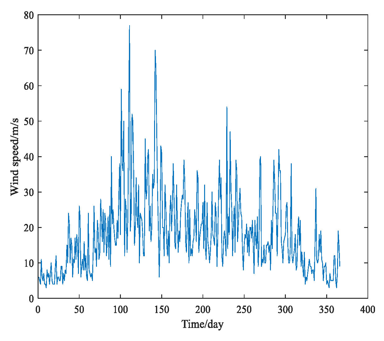
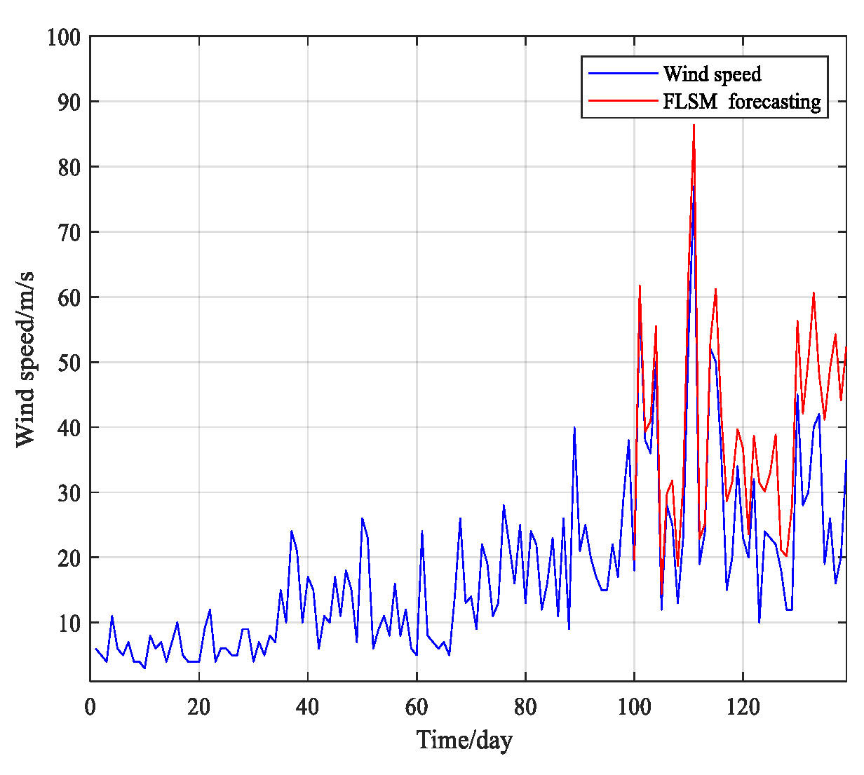
We used the average daily wind speed data from the 2011 actual historical wind speed of Inner Mongolia. The historical wind speed waveform is shown in Figure 2. When the wind speed is too high, it will seriously affect the power grid, so we focused on accurately predicting the time period when the wind speed is high. It can be seen from Figure 2 that the wind speed data began to fluctuate greatly from the 100th day, which was harmful to the power grid, so we chose to start from the 100th forecast. In terms of selecting the prediction steps, the small-data method of the second part was used to calculate the maximum prediction steps. The calculation results are shown in Table 1. The maximum forecast steps were 43 days, we could set the forecast time period from the 100th day to the 140th day. Before using the fLsm iterative forecasting model, we needed to determine whether the wind speed sequence was LRD. Through parameter estimation, we could get the value of H and α (Table 2), satisfying α H > 1 . Finally, the fLsm iterative forecasting model was used to forecast the wind speed sequence, and the forecast result is shown in Figure 3. The specific method flow is shown in Figure 4.
As can be seen from Figure 3, when the prediction steps exceeded nine steps, the prediction error gradually increased, and the prediction data was often larger than the actual data. However, by calculating the maximum prediction steps of 43, its effective prediction steps were much less than the maximum prediction steps.
As fLsm is an infinite variance process and the variance of the wind speed data is not large, if the historical wind speed data is used to estimate the parameters of the fLsm iterative prediction model, a large error will occur. In this section, we used a method of weighting the wind speed data to increase the variance of the data, thereby reducing the error in parameter estimation.
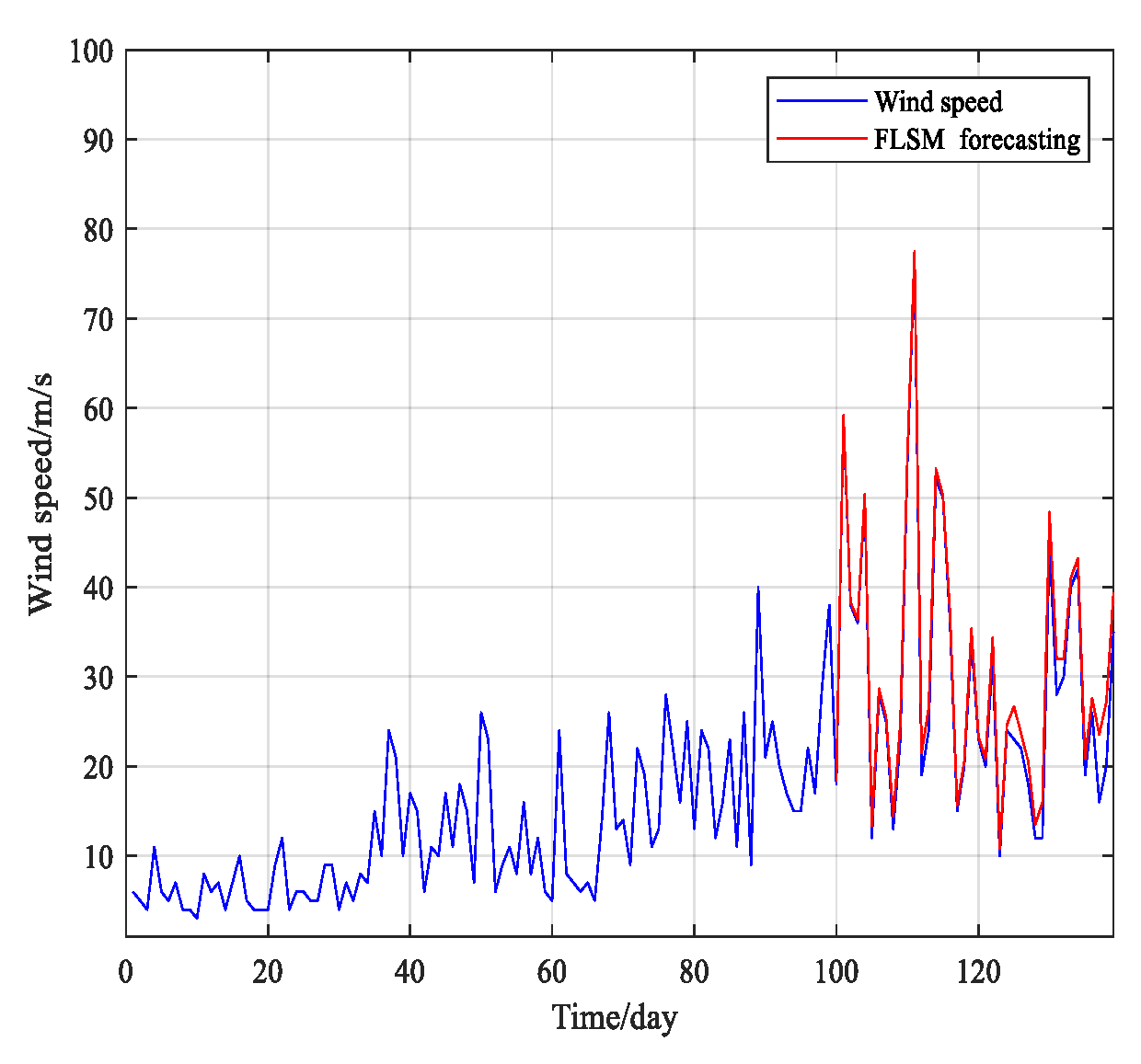
It can be seen from Figure 5 and Figure 6 that the prediction effect of the wind speed weighted data had been significantly improved. Generally speaking, increasing the variance will cause the tail parameter α to decrease. However, it can be seen from Table 2 that the α value of the five-times weighted wind speed data was larger than the α value of the unweighted wind speed data, which indicated that a larger error occurred when modeling the wind speed sequence using the fLsm iterative prediction model. Of course, α H > 1 must be guaranteed when weighting the wind speed data.
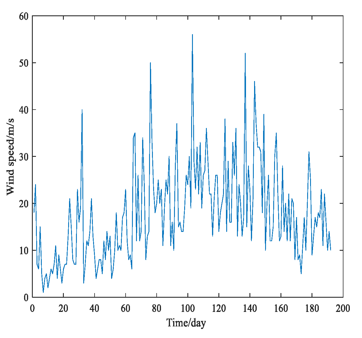
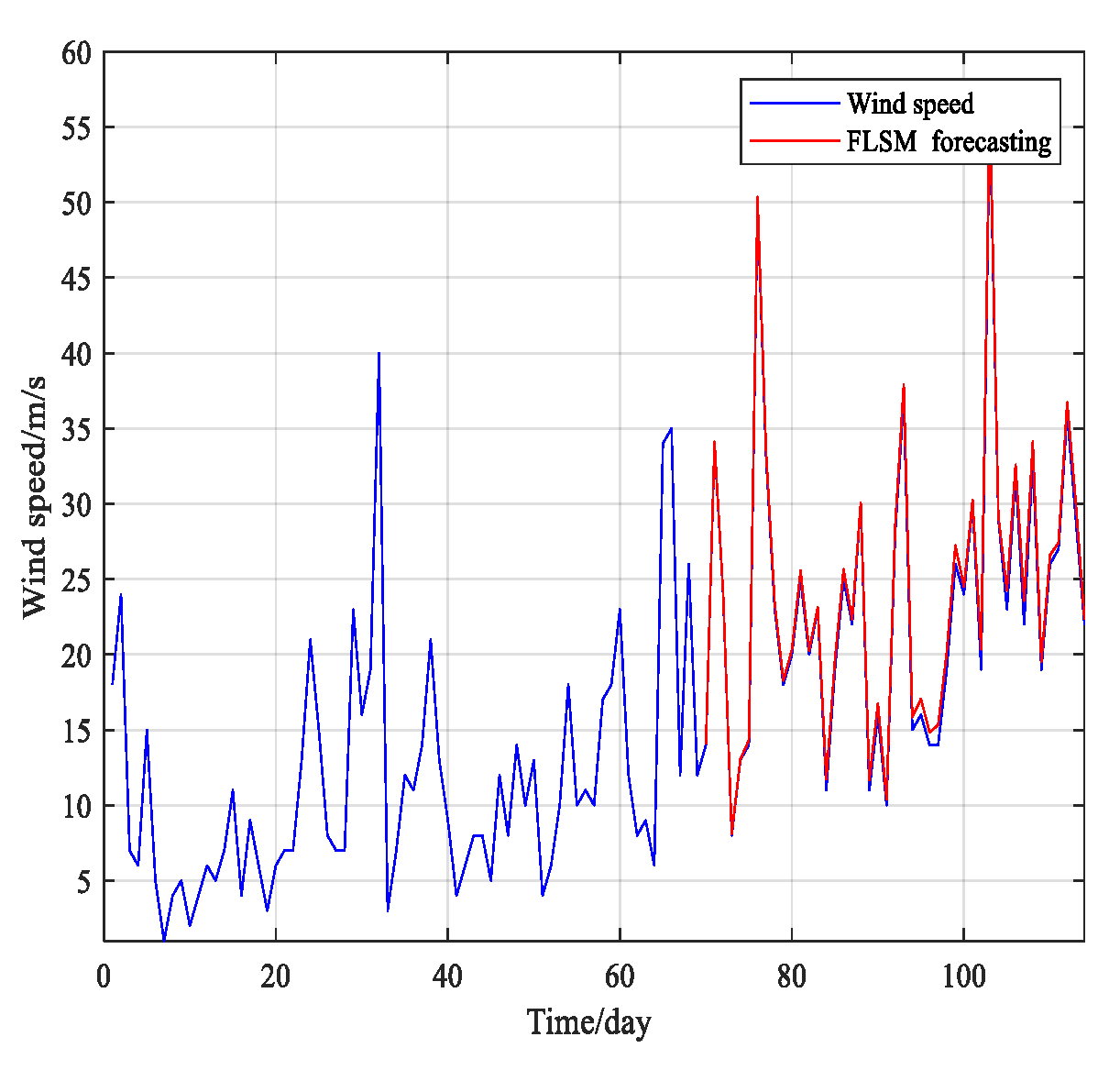
In order to prove the extensiveness of the wind speed prediction model in this paper, we forecasted the wind speed data of Inner Mongolia in 2012. As can be seen from Figure 7, the wind speed data on the 70th day began to fluctuate. We then calculated the maximum number of prediction steps to 45 and set the prediction time period to the 70th to 115th days. After weighting the wind speed data 10 times, the fLsm iterative prediction model was used for prediction in Figure 8. In addition, the fLsm iterative prediction model was compared with the GA-BP neural network, which showed that the wind speed prediction model in this paper had better prediction accuracy.
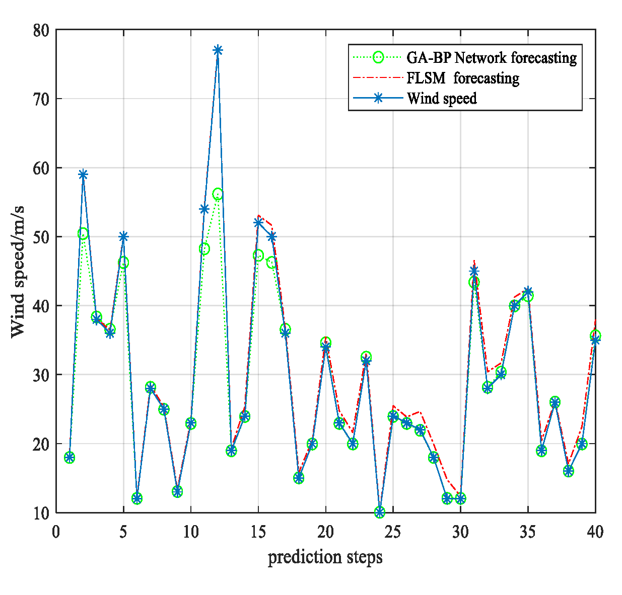
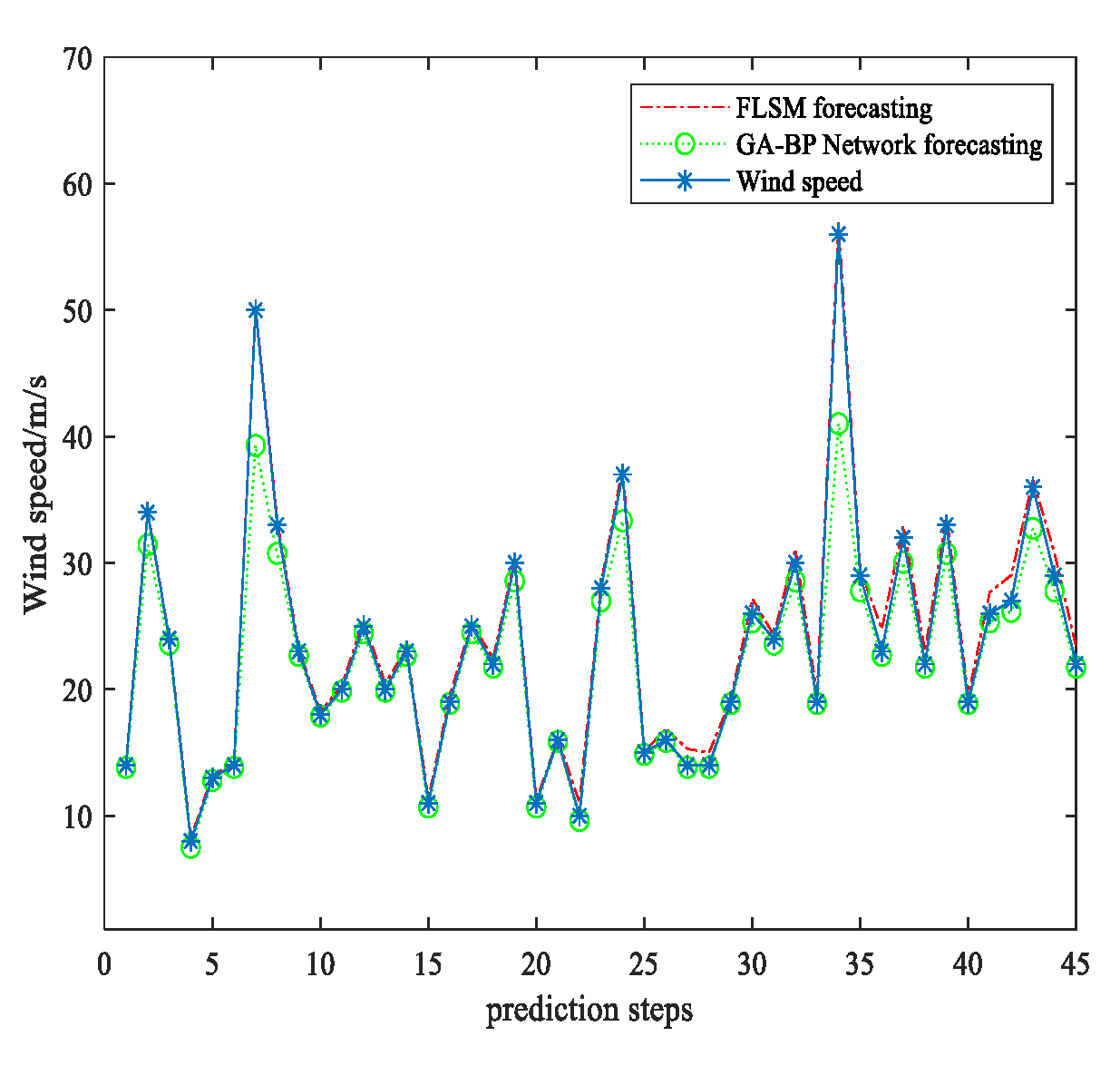
Table 3 lists the maximum and average percentage errors for the two prediction models. As can be seen from the table, the fLsm iterative prediction model had higher prediction accuracy. At the same time, it can be seen from Figure 9 and Figure 10 that the GA-BP neural network had a poor prediction of the peak value, which will lead to the inability to prevent the impact of excessive wind speed on the grid.

6. Relationship between Wind Speed and Wind Power

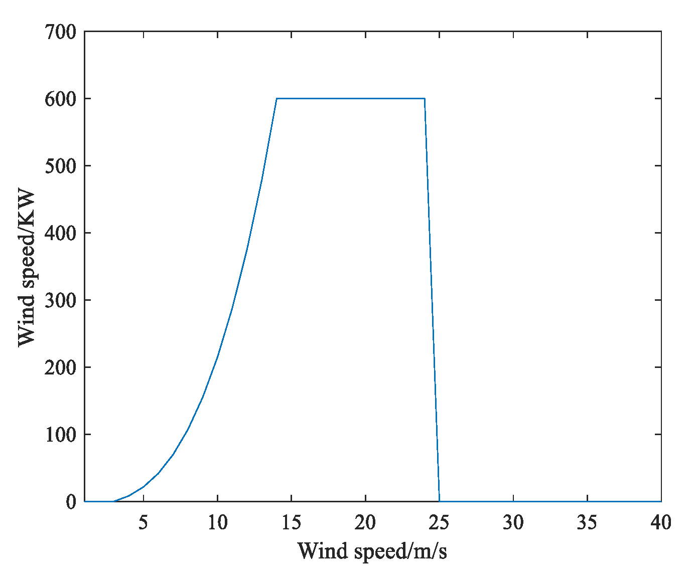
Taking a variable-pitch wind turbine with a single unit capacity of 600 kW as an example, the power characteristics are shown in Figure 11. The cut-in wind speed, cut-out wind speed, and rated wind speed were 3, 50, and 25 m/s, respectively. The raw data of wind power time series could be obtained from the original data of wind speed and power characteristic curve of the wind turbines.
When the wind speed was less than the cut-in wind speed and greater than the cut-out wind speed, the power generation was zero; when the wind speed was equal to the cut-in wind speed, the rated wind speed, and the cut-out wind speed, the power characteristic curve had a significant turning point. When the wind speed was greater than the rated wind speed and less than the cut-out wind speed when the wind speed was out, the generating power was a certain value. Only when the wind speed was greater than the cut-in wind speed and less than the rated wind speed did the generating power, and the wind speed approximate a linear relationship.
P ( v ) = { 0 0 v v i   f p ( v ) v i v v r P r v r v v c 0 v   > v c ,
where P ( v ) is the wind power, P r is the rated power of the generator, vi is the cut-in wind speed, v c is the cut-out wind speed also known as the cut-off wind speed, vr is the rated wind speed, and f p ( v )   is the output characteristic of the wind speed between   v i and vr. Its characteristics can be linear functions, quadratic functions, or cubic functions.

7. Conclusions

(1) Wind speed prediction is of great significance to the stable operation and operating efficiency of the power system. At the same time, it improves the ability of wind farms to participate in market competition.
(2) The wind speed prediction method based on the maximum Lyapunov exponent and fLsm iterative prediction model was effective. Based on the historical wind speed sequence, this paper calculated the maximum prediction steps, weighted the wind speed data, and established an fLsm iterative prediction model. It can be seen from the MATLAB simulation curve that the model can better predict the wind speed and reflect the change of the sequence, which has certain guiding significance. It can be seen from Section 6 that after the conversion of the power characteristic curve, its regularity was partially destroyed, and the regularity of the obtained wind energy was even weaker, which led to a larger forecast error of wind power. Therefore, the wind speed needs to be predicted first, and then the amount of electricity can be calculated.
(3) In practice, wind speed has strong randomness, and some regions may not have LRD. The wind speed sequence of short-range dependent (SRD) has yet to be studied.

Author Contributions

Conceptualization, S.D. and C.C.; Data curation, Y.Y. and H.L.; Formal analysis, W.S. and C.C.; Funding acquisition, W.S.; Investigation, S.D., W.S. and C.C.; Methodology, S.D., W.S. and C.C.; Project administration, W.S. and C.C.; Resources, W.S. and C.C.; Visualization, W.S. and C.C.; Writing–Original draft, S.D.; Writing–Review & editing, W.S. and C.C. All authors have read and agreed to the published version of the manuscript.

Funding

This project was funded by the Natural Science Foundation of Shanghai (Grant No 14ZR1418500).

Conflicts of Interest

The authors declare no conflict of interest.

References

  1. Lei, Y.Z.; Wang, W.S.; Yin, Y.H.; Dai, H.Z. Analysis of wind power value to power system operation. Power Syst. Technol. 2002, 5, 62–66. [Google Scholar]
  2. Shu-Yong, C.H.E.N.; Hui-Zhu, D.A.I.; Xiao-Min, B.A.I.; Xiao-Xin, Z.H.O.U. Reliability model of wind power plants and its application. Proc. -Chin. Soc. Electr. Eng. 2000, 20, 26–29. [Google Scholar]
  3. Ya-Zhou, L.; Wei-Sheng, W.; Yong-Hua, Y. An optimization method for determining wind power penetration limit in power system under static security constraints. Proc. -Chin. Soc. Electr. Eng. 2001, 21, 25–28. [Google Scholar]
  4. Lei, Y.Z.; Wang, W.S.; Yin, Y.H.; Dai, H.Z. Wind power penetration limit calculation based on chance constrained programming. Proc. CSEE 2002, 22, 32–35. [Google Scholar]
  5. Alexiadis, M.C.; Dokopoulos, P.S.; Sahsamanoglou, H.S.; Manousaridis, I.M. Short term forecasting of wind speed and related electrical power. Sol. Energy. 1998, 63, 61–68. [Google Scholar] [CrossRef]
  6. Bossanyi, E.A. Short-term wind prediction using Kalman filters. Wind Eng. 1985, 9, 1–8. [Google Scholar]
  7. Kamal, L.; Jafri, Y.Z. Time series models to simulate and forecast hourly averaged wind speed in Wuetta, Pakistan. Sol. Energy 1997, 61, 23–32. [Google Scholar] [CrossRef]
  8. Kariniotakis, G.N.; Stavrakakis, G.S.; Nogaret, E.F. Wind power forecasting using advanced neural network models. IEEE Trans Energy Convers. 1996, 11, 762–767. [Google Scholar] [CrossRef]
  9. Bayraktar, E.; Poor, H.V.; Rao, R. Prediction and tracking of long-range dependent sequences. Syst. Control Lett. 2005, 34, 1083–1090. [Google Scholar] [CrossRef]
  10. Gao, Y.; Villecco, F.; Li, M.; Song, W. Multi-Scale Permutation Entropy Based on Improved LMD and HMM for Rolling Bearing Diagnosis. Entropy 2017, 19, 176. [Google Scholar] [CrossRef] [Green Version]
  11. Song, W.; Cattani, C.; Chi, C.H. Multifractional Brownian Motion and Quantum-Behaved Particle Swarm Optimization for Short Term Power Load Forecasting: An Integrated Approach. Energy 2020, 194, 116847. [Google Scholar] [CrossRef]
  12. Wanqing, S.; Chen, X.; Cattani, C.; Zio, E. Multifractional Brownian Motion and Quantum-Behaved Partial Swarm Optimization for Bearing Degradation Forecasting. Complexity 2020. [Google Scholar] [CrossRef]
  13. Li, Y.; Song, W.; Wu, F.; Zio, E.; Zhang, Y. Spectral Kurtosis of Choi–Williams Distribution and Hidden Markov Model for Gearbox Fault Diagnosis. Symmetry 2020, 12, 285. [Google Scholar] [CrossRef] [Green Version]
  14. Li, M. Fractal Time Series—A Tutorial Review. Math. Probl. Eng. 2010. [Google Scholar] [CrossRef]
  15. Liu, H.; Song, W.; Li, M.; Kudreyko, A.; Zio, E. Fractional Lévy stable motion: Finite difference iterative Forecasting model. Chaos Solitons Fractals 2020, 133, 109632. [Google Scholar] [CrossRef]
  16. Rosenstein, M.T.; Collins, J.J.; De Luca, C.J. A practical method for calculating largest Lyapunov exponents from small data sets. Phys. D: Nonlinear Phenom. 1993, 65, 117–134. [Google Scholar] [CrossRef]
  17. Kim, H.; Eykholt, R.; Salas, J.D. Nonlinear dynamics, delay time and embedding windows. Phys. D: Nonlinear Phenom. 1999, 127, 48–60. [Google Scholar] [CrossRef]
  18. Tao, H.Y.C. Phase-space reconstruction technology of chaotic attractor based on c-c method. J. Electron. Meas. Instrum. 2012, 26, 425–430. [Google Scholar]
  19. Weron, A.; Burnecki, K.; Mercik, S.; Weron, K. Complete description of all self-similar models driven by Levy stable noise. Phys. Rev. E 2005. [Google Scholar] [CrossRef] [Green Version]
  20. Black, F.; Scholes, M. The pricing of options and corporate liabilities. J. Political Econ. 1973, 81, 637–654. [Google Scholar] [CrossRef] [Green Version]
  21. Jumarie, G. Merton’s model of optimal portfolio in a Black-Scholes market driven by a fractional Brownian motion with short-range dependence. Insur. Math. Econ. 2005, 37, 585–598. [Google Scholar] [CrossRef]
  22. Jumarie, G. On the representation of fractional Brownian motion as an integral with respect to (dt)a. Appl. Math. Lett. 2005, 18, 739–748. [Google Scholar] [CrossRef] [Green Version]
  23. Qin, Y.; Xiang, S.; Chai, Y.; Chen, H. Macroscopic-microscopic attention in LSTM networks based on fusion features for gear remaining life prediction. IEEE Trans. Ind. Electron. 2020. [Google Scholar] [CrossRef]
  24. Wang, X.; Li, K.; Gao, P.; Meng, S. Research on parameter estimation methods for alpha stable noise in a laser gyroscope’s random error. Sensors 2015, 15, 18550–18564. [Google Scholar] [CrossRef] [PubMed] [Green Version]
  25. Ding, Z.; Sun, G.; Guo, M.; Jiang, X.; Li, B.; Liang, S.Y. Effect of phase transition on micro-grinding-induced residual stress. J. Mater. Process. Technol. 2020, 281, 116647. [Google Scholar] [CrossRef]
  26. Zou, H.L.; Yu, Z.G.; Anh, V.; Ma, Y.L. From standard alpha-stable levy motions to horizontal visibility networks: Dependence of multifractal and Laplacian spectrum. J. Stat. Mech. Theory Exp. 2018, 053403. [Google Scholar] [CrossRef]
  27. Song, W.; Li, M.; Li, Y.; Cattani, C.; Chi, C.H. Fractional Brownian motion: Difference iterative forecasting models. Chaos Solitons Fractals 2019, 123, 347–355. [Google Scholar] [CrossRef]
  28. Kogon, S.M.; Manolakis, D.G. Signal modeling with self-similar stable processes: The fractional levy stable motion model. IEEE Trans. Signal Process. 1996, 44, 1006–1010. [Google Scholar] [CrossRef]
  29. Laskin, N.; Lambadaris, I.; Harmantzis, F.C.; Devetsikiotis, M. Fractional levy motion and its application to network traffic modeling. Comput. Netw. 2002, 40, 363–375. [Google Scholar] [CrossRef] [Green Version]
  30. Karasaridis, A.; Hatzinakos, D. Network heavy traffic modeling using stable self-similar processes. Ieee Trans. Commun. 2001, 49, 1203–1214. [Google Scholar] [CrossRef]
  31. Dai, W.; Heyde, C.C. It’s formula with respect to fractional brownian motion and its application. J. Appl. Math. Stoch. Anal. 1996, 9. [Google Scholar] [CrossRef] [Green Version]
  32. Wang, X.T.; Qiu, W.Y.; Ren, F.Y. Option pricing of fractional version of the black-scholes model with hurst exponent h being in (1/3,1/2). Chaos Solitons Fractals 2001, 12, 599–608. [Google Scholar] [CrossRef]
Figure 1. Influence of different characteristic index values on the probability distribution function.
Symmetry 12 00605 g001
Figure 2. 2011 wind speed waveform.
Symmetry 12 00605 g002
Figure 3. Unweighted wind speed predictions.
Symmetry 12 00605 g003
Figure 4. Forecasting process.
Symmetry 12 00605 g004
Figure 5. Five-time weighted wind speed predictions.
Symmetry 12 00605 g005
Figure 6. Ten-time weighted wind speed predictions.
Symmetry 12 00605 g006
Figure 7. 2012 wind speed waveform.
Symmetry 12 00605 g007
Figure 8. 2012 wind speed forecast results.
Symmetry 12 00605 g008
Figure 9. Comparison of prediction effects in 2011.
Symmetry 12 00605 g009
Figure 10. Comparison of prediction effects in 2012.
Symmetry 12 00605 g010
Figure 11. Power curve of a wind power generator.
Symmetry 12 00605 g011
Table 1. 2011 Small-data method parameters.
Parameter NameParameter Value
Average period12
Embedding Dim5
Time delay2
Lyapunov exponent0.0238
Max. prediction steps43
Table 2. Parameters and errors of the three weighting methods.
NameUnweighted5 Weighted10 Weighted
Max error percentage3.73190.44250.1419
H0.75950.75950.7595
α1.79591.82801.6305
var173.7598434417376
Table 3. Errors of the two prediction models.
YearsNameGA-BP NetworkFLSM Forecasting
2011Max error percentage0.27060.1419
2011Mean error percentage0.03500.0304
2012Max error percentage0.26760.1022
2012Mean error percentage0.03780.0282