Article

Numerical Solution of Direct and Inverse Problems for Time-Dependent Volterra Integro-Differential Equation Using Finite Integration Method with Shifted Chebyshev Polynomials

Department of Mathematics and Computer Science, Faculty of Science, Chulalongkorn University, Bangkok 10330, Thailand
*
Author to whom correspondence should be addressed.
Symmetry 2020, 12(4), 497; https://doi.org/10.3390/sym12040497
Submission received: 3 February 2020 / Revised: 2 March 2020 / Accepted: 5 March 2020 / Published: 30 March 2020
(This article belongs to the Special Issue Mesh Methods - Numerical Analysis and Experiments)

Abstract

:
In this article, the direct and inverse problems for the one-dimensional time-dependent Volterra integro-differential equation involving two integration terms of the unknown function (i.e., with respect to time and space) are considered. In order to acquire accurate numerical results, we apply the finite integration method based on shifted Chebyshev polynomials (FIM-SCP) to handle the spatial variable. These shifted Chebyshev polynomials are symmetric (either with respect to the point x = L 2 or the vertical line x = L 2 depending on their degree) over [ 0 , L ] , and their zeros in the interval are distributed symmetrically. We use these zeros to construct the main tool of FIM-SCP: the Chebyshev integration matrix. The forward difference quotient is used to deal with the temporal variable. Then, we obtain efficient numerical algorithms for solving both the direct and inverse problems. However, the ill-posedness of the inverse problem causes instability in the solution and, so, the Tikhonov regularization method is utilized to stabilize the solution. Furthermore, several direct and inverse numerical experiments are illustrated. Evidently, our proposed algorithms for both the direct and inverse problems give a highly accurate result with low computational cost, due to the small number of iterations and discretization.

1. Introduction

An integro-differential equation (IDE) is an equation which contains both derivatives and integrals of an unknown function. Several situations in the branches of science and engineering can be demonstrated by developing mathematical models which are often in the form of IDEs, such as in RLC circuit analysis, the activity of interacting inhibitory and excitatory neurons, the Wilson–Cowan model, and so on; see Reference [1] for more applications. In fact, many of these problems cannot be directly solved, because we may not know all necessary information or an incomplete system may be provided. This has led to the study of both direct and inverse problems for a certain type of one-dimensional IDE involving time, which is called the one-dimensional time-dependent Volterra IDE (TVIDE). Hence, in this study, we investigate the TVIDE of the following form
v t ( x , t ) + L v ( x , t ) = 0 t κ 1 ( x , η ) v ( x , η ) d η + 0 x κ 2 ( ξ , t ) v ( ξ , t ) d ξ + F ( x , t ) ,
for all ( x , t ) ( 0 , L ) × ( 0 , T ] , where x and t represent space and time variables, respectively; L is the spatial linear differential operator of order n; κ 1 ( x , t ) and κ 2 ( x , t ) are the given continuously integrable kernel functions; and v ( x , t ) is an unknown function, which is to be determined subject to prescribed initial and boundary conditions. We remark that, if a forcing term F ( x , t ) of (1) is given, then this problem has only one unknown v ( x , t ) C n , 1 ( [ 0 , L ] × [ 0 , T ] ) to be solved, and it is called a direct problem. In contrast, if the forcing term F ( x , t ) is missing, then this problem has two unknowns F ( x , t ) C ( [ 0 , L ] × [ 0 , T ] ) and v ( x , t ) C n , 1 ( [ 0 , L ] × [ 0 , T ] ) to be solved, and it is called an inverse problem. However, for the inverse problem in this paper, we specifically define the forcing term F ( x , t ) : = β ( t ) f ( x , t ) , where β ( t ) is a missing source function to be retrieved and f ( x , t ) is the given function. We note that (1) has both 0 t κ 1 ( x , η ) v ( x , η ) d η and 0 x κ 2 ( ξ , t ) v ( ξ , t ) d ξ , while several studies in the literature have considered similar problems containing only one of these two terms.
The Volterra IDE containing only an integration term with respect to time arises in many applications, including the compression of poro-viscoelastic media, blow-up problems, analysis of space–time-dependent nuclear reactor dynamics, and so on; see Reference [2]. The existence, uniqueness, and asymptotic behavior of its solution have been discussed in Reference [3]. There are many authors who have studied the numerical solution of this type of problem by using techniques such as the finite element method [2], finite difference method (FDM) [4], collocation methods in polynomial spline [5], the implicit Runge–Kutta–Nyström method [6], the Legendre collocation method [7], and so on.
On the other hand, the Volterra IDE containing only an integration term with respect to space has also been studied in various areas, such as for the one-dimensional viscoelastic problem and one-dimensional heat flow in materials with memory [8], modeling heat/mass diffusion processes, biological species coexisting together with increasing and decreasing rates of growth, electromagnetism, and ocean circulation, among others [9]. Moreover, the existence and uniqueness for this type of Volterra IDE were shown in Reference [8]. Consequently, abundant numerical methods have appeared for finding solutions to this type of Volterra IDE using, for example, spline collocation method [10], collocation method with implicit Runge–Kutta method [11], decomposition method [12], and so on.
However, our problem deals with a Volterra IDE involving both temporal and spatial integrations. There have been no results in the literature regarding the existence and uniqueness of solutions to this type of problem. In this paper, we concentrate on providing a decent numerical procedure to find approximate solutions for both the direct and inverse problems of the proposed TVIDE (1).
Generally, it is well-known that the classification of problems involving differential equations was defined by Hadamard [13] in 1902. Mathematical problems involving differential equations are well-posed if the following conditions hold: existence, uniqueness, and stability. Otherwise, the problem is called ill-posed; this normally occurs in the inverse problem. Even though the initial and boundary conditions are prescribed, it is not sufficient to guarantee that our inverse problem (1) has unique solutions β ( t ) and v ( x , t ) . Hence, additional conditions (e.g., the observation or measurement of data) need to be involved. In practice, there are many kinds of additional conditions; for example, a fixed point of the system, an average time of the system, or an integral of the system. After the additional conditions has been added as an auxiliary condition in our inverse problem (1), we can obtain the existence and uniqueness of β ( t ) and v ( x , t ) . However, the additional condition may contains measurement or observation errors, which may cause the instability in the solutions; namely, a small perturbation in the input data can produce a considerable error, especially for β ( t ) . Thus, some regularization techniques are required to overcome the ill-posedness and stabilize the solution.
There exist many schemes which are generally used to solve both direct and inverse problems of Volterra IDEs, such as the above-mentioned methods. However, those methods utilize the process of approximating differentiation. It is well-known that numerical differentiation is very sensitive to rounding errors, as its manipulation task involves division by a small step-size. On the other hand, the process of numerical integration involves multiplication by a small step-size and, so, it is very insensitive to rounding errors. In recent years, the finite integration method (FIM) has been developed to find approximate solutions of linear boundary value problems for partial differential equations (PDEs). The concept of FIM is to transform a given PDE into an equivalent integral equation, following which a numerical integration method, such as the trapezoid, Simpson, or Newton–Cotes methods (see References [14,15,16]), are applied. In 2018, Boonklurb et al. [17] modified the traditional FIM by using Chebyshev polynomials to solve one- and two-dimensional linear PDEs and obtained a more accurate result compared to the traditional FIMs and FDM. However, their technique [17] has not yet been utilized to overcome the direct and inverse problems of TVIDE, which are the major focuses of this work.
In this paper, we formulate numerical algorithms for solving the direct and inverse problems of TVIDE (1). We manipulate the idea of FIM in Reference [17] by using shifted Chebyshev polynomials, which we call the FIM with shifted Chebyshev polynomials (FIM-SCP), to deal with the spatial variable and use the forward difference quotient to estimate the time derivative. We further apply the Tikhonov regularization method to stabilize our ill-posed problem (1). The rest of the paper is organized as follows. In Section 2, the definition and some basic properties concerning the shifted Chebyshev polynomial are given to construct the shifted Chebyshev integration matrices. The Tikhonov regularization method is also presented in Section 2. In Section 3, we use the FIM-SCP and the forward difference quotient to devise efficient numerical algorithms to find approximate solutions to the direct and inverse problems of (1). Then, we implement our proposed algorithms through several examples, in order to demonstrate their efficiency compared with their analytical solutions. Furthermore, we also display the time convergence rate and CPU time (s) in Section 4. Finally, the conclusion and some directions for future work are given in Section 5.

2. Preliminaries

In this section, we introduce some necessary tools for solving the direct and inverse problems of TVIDE (1): the FIM-SCP and the Tikhonov regularization method.

2.1. Shifted Chebyshev Integration Matrices

We first introduce the definition and some basic properties of shifted Chebyshev polynomials [18], which are used to establish the first- and higher-order shifted Chebyshev integration matrices based on the idea of constructing integration matrices in Reference [17]. However, we slightly modify this idea by instead using a shifted Chebyshev expansion suitable for solving our problem (1) without domain transformation. We give the definition and properties as follows.
Definition 1.
The shifted Chebyshev polynomial of degree n 0 is defined by
S n ( x ) = cos n arccos 2 x L 1 for x [ 0 , L ] .
Note that this shifted Chebyshev polynomial is symmetric, either with respect to the point x = L 2 or the vertical line x = L 2 over [ 0 , L ] , depending on its degree. Next, we provide some important properties of the shifted Chebyshev polynomial, which we use to constructing the shifted Chebyshev integration matrix, as follows.
Lemma 1.
(i) For n N , the zeros of S n ( x ) are symmetrically distributed over [ 0 , L ] and given by
x k = L 2 cos 2 k 1 2 n π + 1 , k { 1 , 2 , 3 , . . . , n } .
(ii) For r N , the r th -order derivatives of S n ( x ) at the endpoint b { 0 , L } are
d r d x r S n ( x ) | x = b = k = 0 r 1 n 2 k 2 2 k + 1 2 b L 1 n + r .
(iii) For x [ 0 , L ] , the single-layer integrations of shifted Chebyshev polynomial S n ( x ) are
S ¯ 0 ( x ) = 0 x S 0 ( ξ ) d ξ = x , S ¯ 1 ( x ) = 0 x S 1 ( ξ ) d ξ = x 2 L x , S ¯ n ( x ) = 0 x S n ( ξ ) d ξ = L 4 S n + 1 ( x ) n + 1 S n 1 ( x ) n 1 2 ( 1 ) n n 2 1 , n { 2 , 3 , 4 , . . . } .
(iv) Let { x k } k = 1 n be a set of zeros of S n ( x ) , the shifted Chebyshev matrix S is defined by
S = S 0 ( x 1 ) S 1 ( x 1 ) S n 1 ( x 1 ) S 0 ( x 2 ) S 1 ( x 2 ) S n 1 ( x 2 ) S 0 ( x n ) S 1 ( x n ) S n 1 ( x n ) .
Then, it has the multiplicative inverse S 1 = 1 n diag ( 1 , 2 , 2 , . . . , 2 ) S .
Next, we use the above definition and properties of shifted Chebyshev polynomials to construct the shifted Chebyshev integration matrices. First, let N be a positive integer and L be a positive real number. Define an approximate solution u ( x ) of a certain differential equation by a linear combination of shifted Chebyshev polynomials S n ( x ) ; that is,
u ( x ) = n = 0 N 1 c n S n ( x ) for x [ 0 , L ] .
Let x k for k { 1 , 2 , 3 , . . . , N } be the interpolated points which are meshed by the zeros of S N ( x ) defined in (2). Substituting each x k into (4), it can be expressed (in matrix form) as
u ( x 1 ) u ( x 2 ) u ( x N ) = S 0 ( x 1 ) S 1 ( x 1 ) S N 1 ( x 1 ) S 0 ( x 2 ) S 1 ( x 2 ) S N 1 ( x 2 ) S 0 ( x N ) S 1 ( x N ) S N 1 ( x N ) c 0 c 1 c N 1 , ,
which is denoted by u = Sc . The unknown coefficient vector can be performed by c = S 1 u . Let us consider the single-layer integration of u ( x ) from 0 to x k , which is denoted by U ( 1 ) ( x k ) ; we obtain
U ( 1 ) ( x k ) = 0 x k u ( ξ ) d ξ = n = 0 N 1 c n 0 x k S n ( ξ ) d ξ = n = 0 N 1 c n S ¯ n ( x k )
for k { 1 , 2 , 3 , . . . , N } or, in matrix form,
U ( 1 ) ( x 1 ) U ( 1 ) ( x 2 ) U ( 1 ) ( x N ) = S ¯ 0 ( x 1 ) S ¯ 1 ( x 1 ) S ¯ N 1 ( x 1 ) S ¯ 0 ( x 2 ) S ¯ 1 ( x 2 ) S ¯ N 1 ( x 2 ) S ¯ 0 ( x N ) S ¯ 1 ( x N ) S ¯ N 1 ( x N ) c 0 c 1 c N 1 .
We denote the above matrix by U ( 1 ) = S ¯ c = S ¯ S 1 u : = Au , where A = S ¯ S 1 : = [ a k i ] N × N is called the first-order shifted Chebyshev integration matrix for the FIM-SCP; that is,
U ( 1 ) ( x k ) = 0 x k u ( ξ ) d ξ = i = 1 N a k i u ( x i ) .
Next, consider the double-layer integration of u ( x ) from 0 to x k , which denoted by U ( 2 ) ( x k ) . We have
U ( 2 ) ( x k ) = 0 x k 0 ξ 2 u ( ξ 1 ) d ξ 1 d ξ 2 = i = 1 N a k i 0 x i u ( ξ 1 ) d ξ 1 = i = 1 N j = 1 N a k i a i j u ( x j )
for k { 1 , 2 , 3 , . . . , N } . It can be written, in matrix form, as U ( 2 ) = A 2 u . Similarly, we can calculate the n-layer integration of u ( x ) from 0 to x k , which is denoted by U ( n ) ( x k ) . Then, we have
U ( n ) ( x k ) = 0 x k 0 ξ 2 u ( ξ 1 ) d ξ 1 d ξ n = i n = 1 N j = 1 N a k i n a i 1 j u ( x j )
for k { 1 , 2 , 3 , . . . , N } , which can be expressed, in matrix form, as U ( n ) = A n u .

2.2. Tikhonov Regularization Method

In this section, we briefly present the idea of the Tikhonov regularization method [19], which is usually applied to stabilize ill-posed problems, such as our inverse problem. Normally, the considered inverse problem can be represented by the system of m linear equations with n unknowns, as
A x = b ϵ ,
where b ϵ is the vector in the right-hand side, which is perturbed by some noise ϵ , and x is the solution of the system (5) after perturbation. Tikhonov regularization replaces the inverse problem (5) by a minimization problem to obtain an efficiently approximate solution, which can be described as
arg min x R n A x b ϵ 2 + λ x 2 ,
where λ > 0 is a regularization parameter balancing the weighting between the two terms of the function and · is the standard Euclidean norm. To reformulate the above minimization problem (6), we obtain
arg min x R n A λ I x b ϵ 0 2 .
Clearly, this is a linear least-square problem in x . Then, the above problem turns out to be the normal equation of the form
A λ I A λ I x = A λ I b ϵ 0 .
To simplify the above equation, the solution x under the regularization parameter λ (denoted by x λ ) can be computed by
x λ = ( A A + λ I ) 1 A b ϵ .
We can see that the accuracy of x λ in (7) depends on the regularization parameter λ , which plays an important role in the calculation: A large regularization parameter may over-smoothen the solution, while a small regularization parameter may lose the ability to stabilize the solution. Therefore, a suitable choice of the regularization parameter λ is very significant for finding a stable approximate solution. There are many approaches for choosing a value of the parameter λ , such as the discrepancy principle criterion, the generalized cross-validation, the L-curve method, and so on. Nevertheless, the regularization parameter λ in this paper is chosen according to Morozov’s discrepancy principle combined with Newton’s method, which has been proposed in Reference [20]. We provide the procedure for calculating the optimal regularization parameter λ below, which can be carried out by the following steps:
  • Step 1: Set n = 0 and give an initial regularization parameter λ 0 > 0 .
  • Step 2: Compute x λ n = ( A A + λ n I ) 1 A b ϵ .
  • Step 3: Compute x λ n = ( A A + λ n I ) 1 x λ n .
  • Step 4: Compute G ( λ n ) = A x λ n b ϵ 2 ϵ 2 .
  • Step 5: Compute G ( λ n ) = 2 λ n A x λ n 2 + 2 λ n 2 x λ n 2 .
  • Step 6: Compute λ n + 1 = λ n G ( λ n ) G ( λ n ) .
  • Step 7: If λ n + 1 λ n < δ for a tolerance δ , end. Else, set n = n + 1 and return to Step 2.  
Therefore, we receive the optimal regularization parameter λ , which is the terminal value λ n obtained from the above procedure. When the regularization parameter λ is fixed as the mentioned optimal value, we can directly obtain the corresponding regularized solution by (7).

3. Numerical Algorithms for Direct and Inverse Problems of TVIDE

In this section, we apply the FIM-SCP described in Section 2.1 to devise the numerical algorithms for solving both the direct and inverse TVIDE problems (1), in order to obtain accurate approximate results. Let u be an approximate solution of v in (1). Then, we have the following linear TVIDE over the domain Ω = ( 0 , L ) × ( 0 , T ] :
u t ( x , t ) + L u ( x , t ) = 0 t κ 1 ( x , η ) u ( x , η ) d η + 0 x κ 2 ( ξ , t ) u ( ξ , t ) d ξ + F ( x , t ) ,
subject to the initial condition
u ( x , 0 ) = ϕ ( x ) , x [ 0 , L ] ,
and the boundary conditions
u ( r ) ( b , t ) = ψ r ( t ) , t [ 0 , T ] ,
for b { 0 , L } and r { 0 , 1 , 2 , . . . , n 1 } , where t and x represent time and space variables, respectively. Additionally, κ 1 , κ 2 , F, ϕ , and ψ r are given continuous functions and L is the spatial linear differential operator of order n defined by L : = i = 0 n p i ( x , t ) d i d x i , where p i ( x , t ) is given and sufficiently smooth.

3.1. Procedure for Solving the Direct TVIDE Problem

First, we linearize (8) by uniformly discretizing the temporal domain into M subintervals with time step τ . Then, we specify (8) at a time t m = m τ for m N and use the first-order forward difference quotient to estimate the time derivative term u t . Next, we replace each x by x k for k { 1 , 2 , 3 , . . . , N } as generated by the zeros of the shifted Chebyshev polynomial S N ( x ) defined in (2). Thus, we have
u m u m 1 τ + L u m = 0 t m κ 1 ( x k , η ) u ( x k , η ) d η + 0 x k κ 2 ( ξ , t m ) u ( ξ , t m ) d ξ + F m ,
where u m = u m ( x k ) = u ( x k , t m ) and F m = F m ( x k ) = F ( x k , t m ) . Next, consider the first integral term with respect to time by letting it be J 1 m ( x k ) , we approximate J 1 m ( x k ) by using the trapezoidal rule. Thus, we approximate J 1 m ( x k ) as
J 1 m ( x k ) : = 0 t m κ 1 ( x k , η ) u ( x k , η ) d η = i = 0 m 1 t i t i + 1 κ 1 ( x k , η ) u ( x k , η ) d η i = 0 m 1 τ 2 κ 1 i ( x k ) u i ( x k ) + κ 1 i + 1 ( x k ) u i + 1 ( x k ) = τ 2 κ 1 0 ( x k ) u 0 ( x k ) + τ i = 1 m 1 κ 1 i ( x k ) u i ( x k ) + τ 2 κ 1 m ( x k ) u m ( x k )
for each x k { x 1 , x 2 , x 3 , . . . , x N } . The above equation can be written, in matrix form, as
J 1 m = τ 2 K 1 0 u 0 + τ i = 1 m 1 K 1 i u i + τ 2 K 1 m u m ,
where each parameter in (12) can be defined as follows:
J 1 m = J 1 m ( x 1 ) , J 1 m ( x 2 ) , J 1 m ( x 3 ) , . . . , J 1 m ( x N ) , u i = u i ( x 1 ) , u i ( x 2 ) , u i ( x 3 ) , . . . , u i ( x N ) , K 1 i = diag κ 1 i ( x 1 ) , κ 1 i ( x 2 ) , κ 1 i ( x 3 ) , . . . , κ 1 i ( x N ) .
Then, we consider the second integral term with respect to space by letting it be J 2 m ( x k ) and using the idea of FIM-SCP (as described in Section 2.1) to approximate it. Then, we obtain
J 2 m ( x k ) : = 0 x k κ 2 ( ξ , t m ) u ( ξ , t m ) d ξ = 0 x k κ 2 m ( ξ ) u m ( ξ ) d ξ i = 1 N a k i κ 2 m ( x i ) u m ( x i )
for each x k { x 1 , x 2 , x 3 , . . . , x N } . The above equation can be written, in matrix form, as
J 2 m = A K 2 m u m ,
where A = S ¯ S 1 is the shifted Chebyshev integration matrix defined in Section 2.1,
J 2 m = J 2 m ( x 1 ) , J 2 m ( x 2 ) , J 2 m ( x 3 ) , . . . , J 2 m ( x N ) , u m = u m ( x 1 ) , u m ( x 2 ) , u m ( x 3 ) , . . . , u m ( x N ) , K 2 m = diag κ 2 m ( x 1 ) , κ 2 m ( x 2 ) , κ 2 m ( x 3 ) , . . . , κ 2 m ( x N ) .
Then, we apply the FIM-SCP (described in Section 2.1) to eliminate all spatial derivatives from (11) by taking the n-layer integral on both sides of (11), to obtain the following equation at the shifted Chebyshev node x k , as defined in (2), as
0 x k . . . 0 ξ 2 u m u m 1 τ + L u m d ξ 1 . . . d ξ n = 0 x k . . . 0 ξ 2 J 1 m + J 2 m + F m d ξ 1 . . . d ξ n .
To simplify the n-layer integration of the spatial derivative terms of L u m , by letting it be Q m ( x k ) and using the technique of integration by parts, we have
Q m ( x k ) : = 0 x k . . . 0 ξ 2 L u m ( ξ 1 ) d ξ 1 . . . d ξ n = 0 x k . . . 0 ξ 2 i = 0 n p i ( ξ 1 , t m ) d i d x i u m ( ξ 1 ) d ξ 1 . . . d ξ n = i = 0 n ( 1 ) i n i 0 x k . . . 0 η 2 p n ( i ) ( η 1 , t m ) u m ( η 1 ) d η 1 . . . d η i + 0 x k i = 0 n 1 ( 1 ) i n 1 i 0 ξ n . . . 0 η 2 p n 1 ( i ) ( η 1 , t m ) u m ( η 1 ) d η 1 . . . d η i d ξ n + 0 x k 0 ξ n i = 0 n 2 ( 1 ) i n 2 i 0 ξ n 1 . . . 0 η 2 p n 2 ( i ) ( η 1 , t m ) u m ( η 1 ) d η 1 . . . d η i d ξ n 1 d ξ n + 0 x k . . . 0 ξ 2 p 0 ( ξ 1 , t m ) u m ( ξ 1 ) d ξ 1 . . . d ξ n + d 1 x k n 1 ( n 1 ) ! + d 2 x k n 2 ( n 2 ) ! + d 3 x k n 3 ( n 3 ) ! + . . . + d n ,
where d 1 , d 2 , d 3 , . . . , d n are the arbitrary constants which emerge from the process of integration by parts. Then, we substitute each x k { x 1 , x 2 , x 3 , . . . , x N } into the above equation and utilize the idea of FIM-SCP. Thus, we can express it, in matrix form, by
Q m = i = 0 n ( 1 ) i n i A i P n ( i ) u m + i = 0 n 1 ( 1 ) i n 1 i A i + 1 P n 1 ( i ) u m + i = 0 n 2 ( 1 ) i n 2 i A i + 2 P n 2 ( i ) u m + + A n P 0 ( 0 ) u m + X n d = j = 0 n i = 0 n j ( 1 ) i n j i A i + j P n j ( i ) u m + X n d ,
where A = S ¯ S 1 is the shifted Chebyshev integration matrix, d = d 1 , d 2 , d 3 , . . . , d N ,
Q m = Q m ( x 1 ) , Q m ( x 2 ) , Q m ( x 3 ) , . . . , Q m ( x N ) , X n = x n 1 , x n 2 , x n 3 , . . . , x 0 for each x i = 1 i ! x 1 i , x 2 i , x 3 i , . . . , x N i , P n j ( i ) = diag p n j ( i ) ( x 1 , t m ) , p n j ( i ) ( x 2 , t m ) , p n j ( i ) ( x 3 , t m ) , . . . , p n j ( i ) ( x N , t m ) .
Finally, we vary all points x k { x 1 , x 2 , x 3 , . . . , x N } in (14) and rearrange them into matrix form by using the FIM-SCP with the derived matrix equations (12), (13), and (15); thus, we obtain
A n u m A n u m 1 τ + Q m = A n J 1 m + A n J 2 m + A n F m
or, factorizing the unknown solution u m explicitly, as
A n + τ j = 0 n i = 0 n j ( 1 ) i n j i A i + j P n j ( i ) τ 2 2 A n K 1 m τ A n + 1 K 2 m u m + X n d = τ 2 2 A n K 1 0 u 0 + τ 2 i = 1 m 1 A n K 1 i u i + A n u m 1 + τ A n F m .
Next, consider the given boundary conditions (10) at the endpoints b { 0 , L } . We can convert them into matrix form by using the linear combination of shifted Chebyshev polynomial (4) in term of the r th -order derivative of u at the iteration time t m and using (3). Then, we have
d r d x r u m ( x ) | x = b = n = 0 N 1 c n m d r d x r S n ( x ) | x = b = ψ r ( t m )
for all r { 0 , 1 , 2 , . . . , n 1 } . We can express the above equation, in matrix form, as
S 0 ( b ) S 1 ( b ) S N 1 ( b ) S 0 ( b ) S 1 ( b ) S N 1 ( b ) S 0 ( n 1 ) ( b ) S 1 ( n 1 ) ( b ) S N 1 ( n 1 ) ( b ) c 0 m c 1 m c N 1 m = ψ 0 ( t m ) ψ 1 ( t m ) ψ n 1 ( t m ) ,
which can be denoted by B c m = Ψ m or B S 1 u m = Ψ m . Finally, we can construct the system of m th iterative linear equations from (16) and (17), which has N + n unknowns containing u m and d , as follows:
H m X n B S 1 0 u m d = E 1 m Ψ m ,
where H m is the coefficient matrix of u m in (16) and E 1 m is the right-hand side column vector of (16). Consequently, the solution u m can be approximated by solving the system (18) starting from the given initial condition (9); that is, u 0 = [ ϕ ( x 1 ) , ϕ ( x 2 ) , ϕ ( x 3 ) , . . . , ϕ ( x N ) ] . Note that, when we would like to find a numerical solution u ( x , t ) at any point x [ 0 , L ] for the terminal time T, we can calculate it by the following formula:
u ( x , T ) = n = 0 N 1 c n m S n ( x ) = s ( x ) c m = s ( x ) S 1 u m ,
where s ( x ) = [ S 0 ( x ) , S 1 ( x ) , S 2 ( x ) , . . . , S N 1 ( x ) ] and u m is the final m t h iterative solution of (18).

3.2. Procedure for Solving Inverse Problem of TVIDE

For the inverse problem in this paper, we specifically define the forcing term F ( x , t ) : = β ( t ) f ( x , t ) , where β ( t ) is a missing source function to be retrieved and f ( x , t ) is the given function. Thus, our considered time-dependent inverse TVIDE problem (1) becomes
u t ( x , t ) + L u ( x , t ) = 0 t κ 1 ( x , η ) u ( x , η ) d η + 0 x κ 2 ( ξ , t ) u ( ξ , t ) d ξ + β ( t ) f ( x , t ) ,
where u is an approximate solution of v and the other parameters are defined as in (8). The initial and boundary conditions of (19) are (9) and (10), which satisfy the compatibility conditions. Now, we remove all spatial derivatives from (19) and use the shifted Chebyshev integration matrix (as explained in Section 2.1). Then, we obtain the following matrix equation, based on the same process as in (16), as
A n + τ j = 0 n i = 0 n j ( 1 ) i n j i A i + j P n j ( i ) τ 2 2 A n K 1 m τ A n + 1 K 2 m u m + X n d τ A n f m β m = τ 2 2 A n K 1 0 u 0 + τ 2 i = 1 m 1 A n K 1 i u i + A n u m 1 ,
where β m = β ( t m ) , f m = [ f ( x 1 , t m ) , f ( x 2 , t m ) , f ( x 3 , t m ) , . . . , f ( x N , t m ) ] and the other parameters in (20) are as defined in Section 3.1. However, the occurrence of missing data is caused by the given conditions being insufficient to ensure a unique solution to our inverse problem. Hence, an additional condition or observed data needs to be involved. Thus, we use an additional condition, regarding the aggregated solution of the system, in the following form:
0 L u ( ξ , t ) d ξ = g ( t ) , t [ 0 , T ] ,
where g ( t ) is the measured data at time t, which probably contains measurement errors. In order to illustrate the realistic phenomena of this problem, we assume that the measurement data of the aggregated solution g ( t ) involves some noise ϵ , which is denoted by g ϵ ( t ) (where g ϵ ( t ) g ( t ) ϵ ) and define the noisy value ϵ by a random variable generated by the Gaussian normal distribution with mean μ = 0 and standard deviation σ = p | g ( t ) | , where p is the percentage of the noise to be input. Then, the additional condition (21) becomes
0 L u ( ξ , t ) d ξ = g ϵ ( t ) , t [ 0 , T ] .
Using the concept of FIM-SCP, the additional condition (22) at time t m can be written, in vector form, as
0 L u m ( ξ ) d ξ = n = 0 N 1 c n m 0 L S n ( ξ ) d ξ = n = 0 N 1 c n m S ¯ n ( L ) d ξ : = z c m = z S 1 u m = g ϵ ( t m ) ,
where z = [ S ¯ 0 ( L ) , S ¯ 1 ( L ) , S ¯ 2 ( L ) , . . . , S ¯ N 1 ( L ) ] and each S ¯ n ( L ) is as defined in Lemma 1(iii). Finally, we can establish the following system of m th iterative linear equations for the inverse TVIDE problem (19) by utilizing (20) and (23), which has N + n + 1 unknown variables including u m , d , and β m , as
H m X n τ A n f m B S 1 0 0 z S 1 0 0 u m d β m = E 2 m Ψ m g ϵ ( t m ) ,
where H m is the coefficient matrix of u m defined in (20) and E 2 m is the right-hand side column vector of (20). Before seeking an approximate solution u m and source term β m , as we have mentioned, we must address that our inverse problem is ill-posed. When a noisy value is input into the system, it may cause a significant error. Hence, we need to stabilize the solution of (24) by employing the Tikhonov regularization method. We denote the linear system (24) by the simplified matrix equation as
R y = b ϵ .
Applying the Tikhonov regularization method (6) in order to filter out the noise in the corresponding perturbed data, we can stabilize the numerical solution (25) by using (7). Thus, we have
y λ = ( R R + λ I ) 1 R b ϵ .
Finally, we can receive the optimal regularization parameter λ by using Morozov’s discrepancy principle combined with Newton’s method, as described in Section 2.2. Thus, we can directly obtain the corresponding regularized solution by (26).

3.3. Algorithms for Solving the Direct and Inverse TVIDE Problems

For computational convenience, we summarize the aforementioned procedures for finding approximate solutions to the direct (8) and inverse (19) TVIDE problems in Section 3.1 and Section 3.2, respectively, as the numerical Algorithms 1 and 2, which are in the form of pseudocode.
Algorithm 1 Numerical algorithm for solving the direct TVIDE problem via FIM-SCP
Input:x, τ , L, T, N, ϕ ( x ) , ψ r ( t ) , p i ( x , t ) , κ 1 ( x , t ) , κ 2 ( x , t ) , and F ( x , t ) .
Output: An approximate solution u ( x , T ) .
1:
Set x k = L 2 cos 2 k 1 2 N π + 1 for k { 1 , 2 , 3 , . . . , N } in descending order.
2:
Compute A , B , S , S ¯ , S 1 , X n , and u 0 .
3:
Set m = 1 and t 1 = τ .
4:
while t m T do
5:
    Compute K 1 m , K 2 m , F m , H m , Ψ m , and E 1 m .
6:
    Find u m by solving the linear system (18).
7:
    Update m = m + 1 .
8:
    Compute t m = m τ .
9:
end while
10:
return Find u ( x , T ) = s ( x ) S 1 u m .
Algorithm 2 Numerical algorithm for solving the inverse TVIDE problem via FIM-SCP
Input:x, p, τ , δ , L, T, N, λ 0 , ϕ ( x ) , g ( t ) , ψ r ( t ) , p i ( x , t ) , κ 1 ( x , t ) , κ 2 ( x , t ) , and f ( x , t ) .
Output: An approximate solution u ( x , T ) and the source terms β ( t m ) at all discretized times.
1:
Set x k = L 2 cos 2 k 1 2 N π + 1 for k { 1 , 2 , 3 , . . . , N } in descending order.
2:
Compute A , B , S , S ¯ , S 1 , X n , A N , and u 0 .
3:
Set m = 1 and t 1 = τ .
4:
while t m T do
5:
    Set the measurement data g ϵ ( t m ) = g ( t m ) + ϵ , where ϵ N ( 0 , p 2 | g ( t m ) | 2 ) .
6:
    Compute K 1 m , K 2 m , f m , H m , Ψ m , E 2 m , R , and b ϵ .
7:
    Set n = 0 .
8:
    do
9:
        Compute y λ n = ( R R + λ n I ) 1 R b ϵ .
10:
        Compute y λ n = ( R R + λ n I ) 1 y λ n .
11:
        Compute G ( λ n ) = R y λ n b ϵ 2 ϵ 2 .
12:
        Compute G ( λ n ) = 2 λ n R y λ n 2 + 2 λ n 2 y λ n 2 .
13:
        Compute λ n + 1 = λ n G ( λ n ) G ( λ n ) .
14:
        Update n = n + 1 .
15:
    while λ n λ n 1 δ
16:
    Set the optimal regularization parameter λ = λ n .
17:
    Find u m and β m by explicitly solving y λ using the matrix equation (7).
18:
    Update m = m + 1 .
19:
    Compute t m = m τ .
20:
end while
21:
return Find u ( x , T ) = s ( x ) S 1 u m .

4. Numerical Experiments

In this section, we implement our devised numerical algorithms for solving the direct and inverse TVIDE problems through several examples, in order to demonstrate the efficiency and accuracy of the solutions obtained by proposed methods. Examples 1 and 2 are used to examine Algorithm 1 for the direct TVIDE problems (8). Examples 3 and 4 are inverse TVIDE problems (19), as solved by Algorithm 2. Additionally, time convergence rates and CPU times(s) for each example are presented to indicate the computational cost and time. The time convergence rate is defined by Rate = lim t m T u ( t m + 1 ) u ( t m + 1 ) u ( t m ) u ( t m ) , where T is the terminal time, t m is a partitioned time contained in [ 0 , T ] , u ( t m ) is the exact solution at time t m , u ( t m ) is the numerical solution at time t m , and · is the l norm. Graphical solutions of each example are also depicted. Our numerical algorithms were implemented using the MatLab R2016a software, run on a Intel(R) Core(TM) i7-6700 CPU @ 3.40 GHz computer system.
Example 1.
Consider the following direct TVIDE problem, which consists of a second-order derivative with constant coefficient for x ( 0 , 1 ) and t ( 0 , T ] :
u t + u x x + u = 0 t 2 e x u ( x , η ) d η + 0 x ( ξ + t ) u ( ξ , t ) d ξ + F ( x , t ) ,
where
F ( x , t ) = t e x ( t 2 3 t + t x 1 ) ,
subject to the homogeneous initial condition u ( x , 0 ) = 0 for x [ 0 , 1 ] and the Dirichlet boundary conditions u ( 0 , t ) = t and u ( 1 , t ) = t e for t [ 0 , T ] . The analytical solution of this problem is u ( x , t ) = t e x .
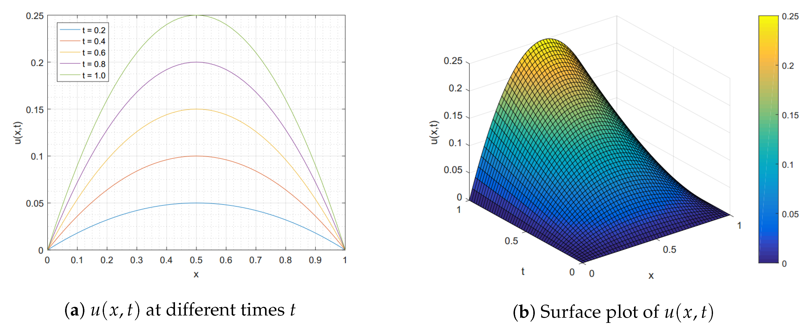
In the numerical testing based on Algorithm 1, we first took the double-layer integral of both sides of (27) and transformed it into matrix form (16). Then, we obtained the approximate solutions u ( x , T ) for this problem (27) by applying the numerical Algorithm 1. The accuracy of our obtained approximate results was measured by the mean absolute error, which compared it to the analytical solution at different values of x { 0 . 1 , 0 . 3 , 0 . 5 , 0 . 7 , 0 . 9 } and the terminal time T = 1 , as shown in Table 1. From Table 1, we observe that, when the partitioning number of the temporal domain M was fixed and nodal numbers N were increasingly varied, then the accuracy was significantly improved. Similarly, for a fixed nodal number N but various time partitioning numbers M, the accuracy results were also significantly improved. Moreover, the convergence rates with respect to the time in Algorithm 1 were estimated for various numbers of the time partition ( M { 5 , 10 , 15 , 20 , 25 } ) for the spatial points N = 10 , as shown in Table 2. We can notice, from Table 2, that these time convergence rates for the norm indeed approached linear convergence for T { 5 , 10 , 15 } . The computational cost, in terms of CPU times (s), is also displayed in Table 2. Finally, a graph of our approximate solutions u ( x , t ) for different times t and the surface plot of the solution under the parameters N = 20 , M = 20 , and T = 1 are depicted in Figure 1.
Example 2.
Consider the following direct TVIDE problem, which consists of a third-order derivative with variable coefficient for x ( 0 , 1 ) and t ( 0 , T ] :
u t + t u x x x + cos ( x ) u x x = 0 t 2 x 1 u ( x , η ) d η + 0 x 6 t ξ 1 u ( ξ , t ) d ξ + F ( x , t ) ,
where
F ( x , t ) = x x 2 + x t 2 ( 3 x + 1 ) 2 t cos ( x ) ,
subject to the initial condition u ( x , 0 ) = 0 for x [ 0 , 1 ] and the boundary conditions u ( 0 , t ) = 0 , u ( 1 , t ) = 0 , and u ( 0 , t ) = t for t [ 0 , T ] . The analytical solution of this problem is u ( x , t ) = ( x x 2 ) t .
We test the efficiency and accuracy of the proposed Algorithm 1 via the problem (28). First, we took a triple-layer integral on both sides of (28) and utilized the shifted Chebyshev integration matrix to transform it into matrix form (16). Next, we implemented Algorithm 1 to obtain numerical solutions u ( x , T ) for this problem (28). Table 3 shows the precision of our obtained approximate results at different values of x { 0 . 1 , 0 . 3 , 0 . 5 , 0 . 7 , 0 . 9 } and at the terminal time T = 1 , through the mean absolute error. We can see that the accuracy was significantly improved according to an increase in the number of both the partitioning space and time domains. However, we observe that, in the case of fixed N, when M was increased, the mean absolute errors provide accurate results with a lower computational number M. Furthermore, the time convergence rates concerning the norm and CPU times (s) are demonstrated in Table 4, under various values of M ( M { 5 , 10 , 15 , 20 , 25 } ) and final times T ( T { 5 , 10 , 15 } ). The graphical solutions for u ( x , t ) in both one and two dimensions are shown in Figure 2.
Example 3.
Consider the following inverse TVIDE problem, which consists of a second-order derivative with constant coefficient and a continuous forcing function f ( x , t ) for x ( 0 , 1 ) and t ( 0 , T ] :
u t u x x + 2 u = 0 t 2 ln ( x ) u ( x , η ) d η + 0 x e ξ u ( ξ , t ) d ξ + β ( t ) f ( x , t ) ,
where
f ( x , t ) = e 2 t 1 + t x + e x + t e x ( 2 e x + t ) t ln x ,
subject to the initial condition u ( x , 0 ) = e x for x [ 0 , 1 ] and the boundary conditions u ( 0 , t ) = t + 1 and u ( 1 , t ) = t + e for t [ 0 , T ] . The additional condition, in terms of the aggregated solution of the system, is g ( t ) = t + e 1 . The analytical solutions of this problem are u ( x , t ) = t + e x and β ( t ) = e 2 t .
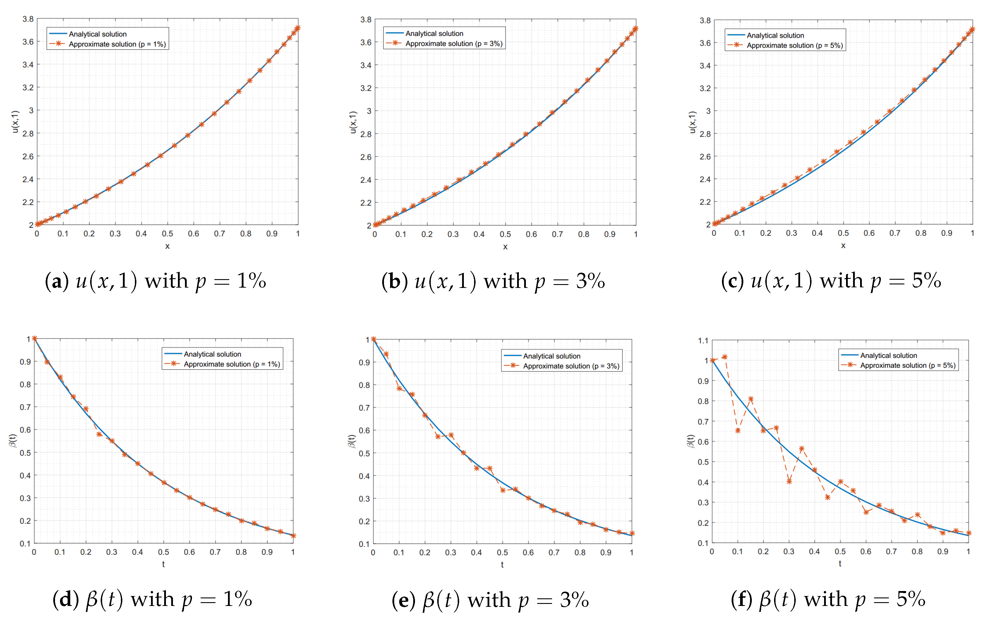
Implementing the numerical Algorithm 2 by taking the double-layer integral of both sides of (29) and transforming it into matrix form (24), we obtained the approximate solutions u ( x , 1 ) and β ( t ) for this problem (29). As the additional condition was measurement data, there may be an error in the measurement. Therefore, we perturbed the additional condition g ( t ) with a percentage p of the noise ( p { 0 % , 1 % , 3 % , 5 % } ). In Table 5, we show the accuracy of the solutions u ( x , 1 ) and β ( t ) , in terms of the mean absolute error, respectively, denoted by E u = 1 N i = 1 N | u i u i | and E β = 1 M j = 1 M | β j β j | , and the values of the optimal regularization parameters λ at time t = 1 with various M = N { 5 , 10 , 15 , 20 } . From Table 5, we can observe that the optimal regularization parameters λ were close to zero and the mean absolute errors for both E u and E β significantly increased with an increasing percentage p of the perturbation. Furthermore, we used the regularization parameter λ = 0 to explore the rates of convergence with respect to the norm and CPU times (s) for M = N { 5 , 10 , 15 , 20 } with the final times T { 1 , 2 , 3 } as shown in Table 6. The graphical solutions of the perturbed functions u ( x , 1 ) and β ( t ) for p { 1 % , 3 % , 5 % } are depicted in Figure 3.
Example 4.
Consider the following inverse TVIDE problem, which consists of a second-order derivative with variable coefficient and the piecewise forcing function f ( x , t ) for x ( 0 , 1 ) and t ( 0 , T ] :
u t + u x x + u x cos ( x t ) u = 0 t 2 sin ( x ) u ( x , η ) d η 0 x 3 t cos ( ξ ) u ( ξ , t ) d ξ + β ( t ) f ( x , t ) ,
where
f ( x , t ) = 1 2 2 t cos ( 2 x ) + t sin ( 2 x ) + ( t cos ( x t ) + 1 ) sin 2 x , 0 < t T 3 , 1 3 2 t cos ( 2 x ) + t sin ( 2 x ) + ( t cos ( x t ) + 1 ) sin 2 x , T 3 < t 2 T 3 , 1 4 2 t cos ( 2 x ) + t sin ( 2 x ) + ( t cos ( x t ) + 1 ) sin 2 x , 2 T 3 < t T ,
subject to the initial condition u ( x , 0 ) = 0 for x [ 0 , 1 ] and the Dirichlet boundary conditions u ( 0 , t ) = 0 and u ( 1 , t ) = t sin 2 ( 1 ) for t [ 0 , T ] . The additional condition, in terms of the aggregated solution of the system, is g ( t ) = t 4 ( 2 s i n ( 2 ) ) + e t . The analytical solutions of this problem are u ( x , t ) = t sin 2 ( x ) and
β ( t ) = 2 , 0 < t T 3 , 3 , T 3 < t 2 T 3 , 4 , 2 T 3 < t T .
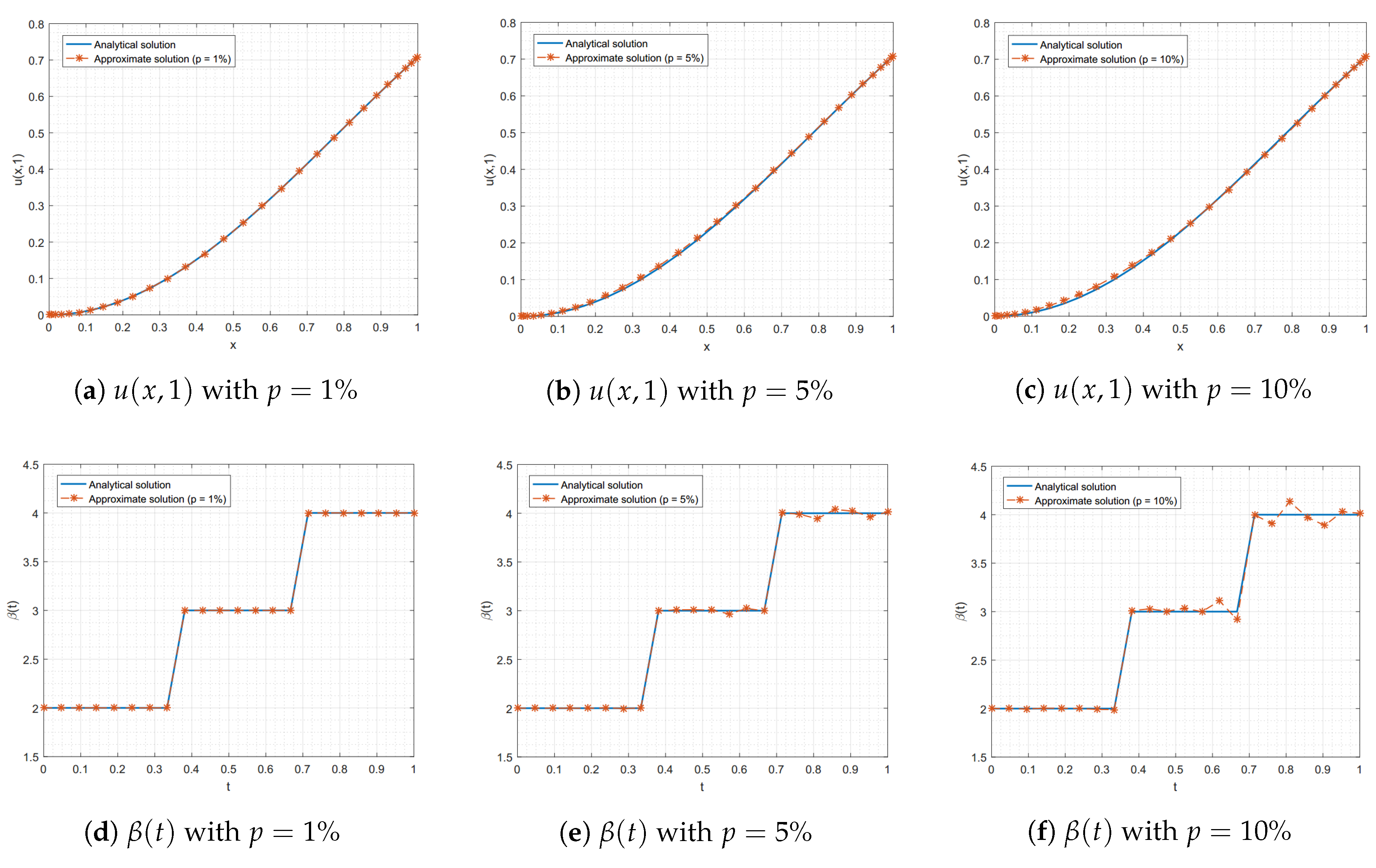
Based on the numerical Algorithm 2, we took the double-layer integral to both sides of (30) and transformed it into matrix form (24). We obtained the approximate solutions u ( x , 1 ) and β ( t ) for (29) by implementing Algorithm 2. Table 7 shows the accuracy of the solutions u ( x , 1 ) and β ( t ) obtained by our numerical algorithm, in terms of the mean absolute errors E u and E β , as well as the values of the optimal regularization parameter λ at time t = 1 with the noisy percentage p { 0 % , 1 % , 5 % , 10 % } under various M = N { 6 , 9 , 12 , 15 } . Although this problem had the piecewise forcing term f ( x , t ) , our Algorithm 2 perfectly performed in providing accurate results, as shown in Table 7. The time convergence rates concerning the norm and CPU times (s) are shown in Table 8, under various numbers of M { 6 , 9 , 12 , 15 , 18 } with the final times T { 1 , 2 , 3 } . The graphical perturbed solutions u ( x , 1 ) and β ( t ) for p { 1 % , 5 % , 10 % } are shown in Figure 4.

5. Conclusions and Discussion

In this paper, we utilized FIM-SCP combined with the forward difference quotient to create efficient and accurate numerical algorithms for solving the considered direct and inverse TVIDE problems. According to the numerical examples in Section 4, we have demonstrated the performance of our proposed Algorithm 1 for seeking the approximate solutions of direct TVIDE problems in Examples 1 and 2. We can see that, for Example 1—which involved a second-order derivative with constant coefficients—Algorithm 1 provided an accurate result. Furthermore, for a problem involving a higher-order derivative with variable coefficients, it still provided high accuracy, in terms of solutions, as demonstrated in Example 2. Moreover, we handled inverse TVIDE problems using Algorithm 2, the effectiveness of which was illustrated in Examples 3 and 4. We used the Tikhonov regularization method to deal with the instability of the inverse problem; it can be seen that, in the examples, the regularization parameter λ was close to zero. Algorithm 2 could handle both continuous and piecewise-defined forcing terms with high accuracy, as demonstrated in Examples 3 and 4. Furthermore, when we perturbed the problems by adding noisy values, our Algorithm 2 still overcame the noise and provided approximate results that approached the analytical solutions. We further notice that our presented methods provide high accuracy, even when using only a small number of nodal points. Evidently, when we decrease the time step, they will furnish more accurate results. The rates of convergence with respect to time (based on the norm) of our methods were observed to be linear. Finally, we also depicted the computational times for each example. However, we realize that there exist no theoretical error analysis results for the proposed numerical algorithms. Thus, our future research will study the error analysis, in order to find theories for order of accuracy and rate of convergence for our method. Another interesting direction for our future work is to extend our techniques to solve other types of IDEs and non-linear IDEs.

Author Contributions

Conceptualization, R.B., A.D., and P.G.; methodology, R.B. and A.D.; software, A.D. and P.G.; validation, R.B., A.D., and P.G.; formal analysis, R.B.; investigation, A.D. and P.G.; writing—original draft preparation, A.D. and P.G.; writing—review and editing, R.B.; visualization, A.D. and P.G.; supervision, R.B.; project administration, R.B.; funding acquisition, R.B. All authors have read and agreed to the published version of the manuscript.

Acknowledgments

The authors would like to thank the reviewers for their thoughtful comments and efforts towards improving our manuscript.

Conflicts of Interest

The authors declare no conflict of interest.

Abbreviations

The following abbreviations are used in this manuscript:
FDMfinite difference method
FIMfinite integration method
FIM-SCPfinite integration method with shifted Chebyshev polynomial
IDEintegro-differential equation
PDEpartial differential equation
TVIDEtime-dependent Volterra integro-differential equation

References

  1. Zill, D.G.; Wright, W.S.; Cullen, M.R. Differential Equations with Boundary-Value Problem, 8th ed.; Brooks/Cole, Cengang Learning: Boston, MA, USA, 2013. [Google Scholar]
  2. Yanik, E.G.; Fairweather, G. Finite element methods for parabolic and hyperbolic partial integro–differential equations. Nonlinear Anal. 1988, 12, 785–809. [Google Scholar] [CrossRef]
  3. Engle, H. On Some Parabolic Integro–Differential Equations: Existence and Asymptotics of Solution; Lecture Notes in Mathematics, Springer: Berlin, Germany, 1983. [Google Scholar]
  4. Tang, T. A finite difference scheme for partial integro–differential equations with a weakly singular kernel. Appl. Numer. Math. 1993, 11, 309–319. [Google Scholar] [CrossRef]
  5. Aguilar, M.; Brunner, H. Collocation methods for second–order Volterra integro–differential equations. Appl. Numer. Math. 1988, 4, 455–470. [Google Scholar] [CrossRef]
  6. Brunner, H. Implicit Runge–Kutta–Nyström methods for general second–order Volterra integro–differential equations. Comput. Math. Appl. 1987, 14, 549–559. [Google Scholar] [CrossRef] [Green Version]
  7. Jiang, Y.J. On spectral methods for Volterra-type integro–differential equations. J. Comput. Appl. Math. 2009, 230, 333–340. [Google Scholar] [CrossRef] [Green Version]
  8. Burton, T.A. Volterra Integral and Differential Equations; Academic Press: New York, NY, USA, 1983. [Google Scholar]
  9. Rahman, M. Integral Equations and Their Applications; WIT Press: Southampton, UK, 2007. [Google Scholar]
  10. Hu, Q. Stieltjes derivatives and beta–polynomial spline collocation for Volterra integro–differential equations with singularities. SIAM J. Numer. 1996, 33, 208–220. [Google Scholar] [CrossRef]
  11. Brunner, H. Superconvergence in collocation and implicit Runge–Kutta methods for Volterra–type integral equations of the second kind. Internet Schriftenreihe Numer. Math. 1980, 53, 54–72. [Google Scholar]
  12. El-Sayed, S.M.; Kaya, D.; Zarea, S. The decomposition method applied to solve high–order linear Volterra–Fredholm integro–differential equations. Internet J. Nonlinear Sci. Numer. Simulat. 2004, 5, 105–112. [Google Scholar] [CrossRef]
  13. Kabanikhin, S.I. Definitions and examples of inverse and ill–posed problems. J. Inverse Ill-Pose Probl. 2008, 16, 317–357. [Google Scholar] [CrossRef]
  14. Wen, P.H.; Hon, Y.C.; Li, M.; Korakianitis, T. Finite integration method for partial differential equations. Appl. Math. Model. 2013, 37, 10092–10106. [Google Scholar] [CrossRef]
  15. Li, M.; Chen, C.S.; Hon, Y.C.; Wen, P.H. Finite integration method for solving multi–dimensional partial differential equations. Appl. Math. Model. 2015, 39, 4979–4994. [Google Scholar] [CrossRef]
  16. Li, M.; Tian, Z.L.; Hon, Y.C.; Chen, C.S.; Wen, P.H. Improved finite integration method for partial differential equations. Eng. Anal. Bound. Elem. 2016, 64, 230–236. [Google Scholar] [CrossRef]
  17. Boonklurb, R.; Duangpan, A.; Treeyaprasert, T. Modified finite integration method using Chebyshev polynomial for solving linear differential equations. J. Numer. Ind. Appl. Math. 2018, 12, 1–19. [Google Scholar]
  18. Rivlin, T.J. Chebyshev Polynomials, From Approximation Theory to Algebra and Number Theory, 2nd ed.; John Wiley and Sons: New York, NY, USA, 1990. [Google Scholar]
  19. Tikhonov, A.N.; Goncharsky, A.V.; Stepanov, V.V.; Yagola, A.G. Numerical Methods for the Solution of Ill–Posed Problems; Springer: Dordrecht, The Netherlands, 1995. [Google Scholar]
  20. Sun, Y. Indirect boundary integral equation method for the Cauchy problem of the Laplace equation. J. Sci. Comput. 2017, 71, 469–498. [Google Scholar] [CrossRef]
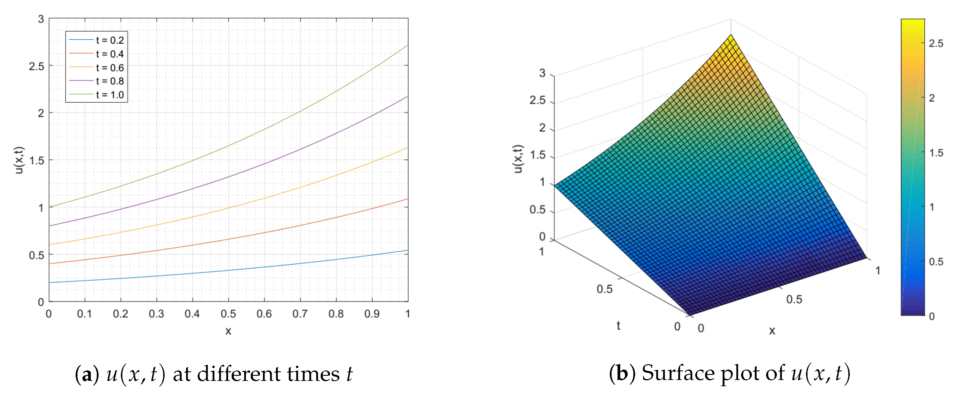
Figure 1. The graphical results of Example 1 for N = 20 , M = 20 , and T = 1 .
Symmetry 12 00497 g001
Figure 2. The graphical results of Example 2 for N = 20 , M = 20 , and T = 1 .
Symmetry 12 00497 g002
Figure 3. The graphical results of u ( x , 1 ) and β ( t ) for Example 3 with N = 30 and M = 20 .
Symmetry 12 00497 g003
Figure 4. The graphical results u ( x , T ) and β ( t ) for Example 4 with N = 30 and M = 21 .
Symmetry 12 00497 g004
Table 1. Mean absolute errors between exact and numerical solutions of u ( x , 1 ) for Example 1.
x M = 20 N = 12
N = 8 N = 10 N = 12 M = 11 M = 13 M = 15
0.1 1.6855 × 10 5 1.1723 × 10 8 1.0208 × 10 10 2.3823 × 10 7 5.0060 × 10 9 3.3268 × 10 11
0.3 4.3851 × 10 5 3.0501 × 10 8 2.6554 × 10 10 6.1976 × 10 7 1.3024 × 10 8 8.6539 × 10 11
0.5 5.3554 × 10 5 3.7247 × 10 8 3.2429 × 10 10 7.5684 × 10 7 1.5904 × 10 8 1.0567 × 10 10
0.7 4.2555 × 10 5 2.9599 × 10 8 2.5767 × 10 10 6.0140 × 10 7 1.2638 × 10 8 8.3964 × 10 11
0.9 1.5864 × 10 5 1.1034 × 10 8 9.6049 × 10 11 2.2419 × 10 7 4.7112 × 10 9 3.1289 × 10 11
Table 2. Time convergence rates and CPU times (s) for Example 1 by Algorithm 1 with N = 10 .
M T = 5 T = 10 T = 15
u u RateTime(s) u u RateTime(s) u u RateTime(s)
5 4.298 × 10 12 1.45840.0465 8.565 × 10 12 1.50760.0456 1.262 × 10 11 1.51120.0469
10 4.318 × 10 12 1.24990.0487 8.576 × 10 12 1.28630.0469 1.276 × 10 11 1.30400.0485
15 4.309 × 10 12 1.17230.0495 8.547 × 10 12 1.20080.0481 1.275 × 10 11 1.21350.0501
20 4.311 × 10 12 1.13270.0506 8.533 × 10 12 1.15550.0516 1.277 × 10 11 1.16570.0535
25 1.135 × 10 12 1.13530.0521 8.540 × 10 12 1.12720.0538 1.277 × 10 11 1.13650.0553
Table 3. Mean absolute errors between exact and numerical solutions of u ( x , 1 ) for Example 2.
x M = 10 N = 10
N = 8 N = 10 N = 12 M = 5 M = 10 M = 15
0.1 3.5098 × 10 10 5.0498 × 10 13 1.6695 × 10 14 5.1849 × 10 13 5.0498 × 10 13 4.9435 × 10 13
0.3 1.0060 × 10 9 1.1285 × 10 12 4.1411 × 10 14 1.1544 × 10 12 1.1285 × 10 12 1.0850 × 10 12
0.5 1.0780 × 10 9 1.4543 × 10 12 5.1958 × 10 14 1.4672 × 10 12 1.4543 × 10 12 1.3845 × 10 12
0.7 1.0237 × 10 9 1.1625 × 10 12 4.5908 × 10 14 1.1572 × 10 12 1.1625 × 10 12 1.0923 × 10 12
0.9 3.1567 × 10 10 5.2400 × 10 13 2.0983 × 10 14 5.1567 × 10 13 5.2400 × 10 13 4.9050 × 10 13
Table 4. Time convergence rates and CPU times (s) for Example 2 by Algorithm 1 with N = 10 .
M T = 5 T = 10 T = 15
u u RateTime(s) u u RateTime(s) u u RateTime(s)
5 1.426 × 10 12 1.02410.0524 1.620 × 10 12 1.04890.0531 3.549 × 10 12 1.37200.0535
10 1.533 × 10 12 1.03340.0577 1.635 × 10 12 1.02780.0576 1.874 × 10 12 1.10350.0576
15 1.426 × 10 12 1.02080.0597 1.664 × 10 12 1.02430.0585 1.806 × 10 12 1.02940.0598
20 1.476 × 10 12 1.02230.0609 1.609 × 10 12 1.02100.0610 1.537 × 10 12 1.02030.0620
25 1.496 × 10 12 1.01650.0619 1.488 × 10 12 1.01820.0638 1.276 × 10 12 1.00790.0641
Table 5. Mean absolute errors of u ( x , 1 ) and β ( t ) for optimal regularization parameter λ of Example 3.
M = N p = 0 % p = 1 %
λ E u E β λ E u E β
5 6.22 × 10 14 1.6609 × 10 5 7.9997 × 10 7 3.11 × 10 12 1.1372 × 10 4 4.1098 × 10 4
10 2.38 × 10 18 3.9844 × 10 13 1.0459 × 10 12 2.20 × 10 13 3.4011 × 10 4 8.8853 × 10 4
15 1.02 × 10 17 9.9950 × 10 14 1.6384 × 10 13 9.17 × 10 12 7.8857 × 10 4 7.0288 × 10 4
20 2.14 × 10 18 2.9774 × 10 13 1.7125 × 10 13 4.33 × 10 14 1.9024 × 10 4 1.3201 × 10 3
M = N p = 3 % p = 5 %
λ E u E β λ E u E β
5 8.80 × 10 11 1.2533 × 10 3 8.3870 × 10 3 8.61 × 10 12 2.2805 × 10 3 1.0964 × 10 2
10 6.64 × 10 11 3.7067 × 10 3 9.5414 × 10 3 1.11 × 10 11 5.0047 × 10 3 2.7003 × 10 2
15 1.09 × 10 12 8.4361 × 10 3 7.0094 × 10 3 8.79 × 10 12 3.2925 × 10 2 3.2201 × 10 2
20 8.61 × 10 12 3.3382 × 10 3 1.3582 × 10 2 1.40 × 10 13 1.0214 × 10 2 3.8774 × 10 2
Table 6. Time convergence rates and CPU times (s) for Example 3 by Algorithm 2 with N = 10 .
M T = 1 T = 2 T = 3
u u RateTime(s) u u RateTime(s) u u RateTime(s)
5 8.495 × 10 13 1.00460.0667 9.130 × 10 13 1.02030.0655 3.602 × 10 12 1.66440.0662
10 8.131 × 10 13 0.99700.0679 8.659 × 10 13 1.00420.0667 2.456 × 10 12 1.24090.0673
15 7.851 × 10 13 0.99650.0684 8.362 × 10 13 1.00010.0675 1.731 × 10 12 1.13550.0693
20 8.344 × 10 13 1.00030.0716 7.829 × 10 13 0.99670.0722 2.928 × 10 12 1.09560.0720
25 8.362 × 10 13 1.00030.0776 8.686 × 10 13 1.00220.0766 2.134 × 10 12 1.06990.0751
Table 7. Mean absolute errors of u ( x , 1 ) and β ( t ) for optimal regularization parameter λ of Example 4.
M = N p = 0 % p = 1 %
λ E u E β λ E u E β
6 1.25 × 10 14 6.4987 × 10 6 18123 × 10 4 2.60 × 10 12 7.8604 × 10 6 1.8959 × 10 4
9 7.41 × 10 17 2.8057 × 10 9 7.1782 × 10 9 3.45 × 10 10 1.2932 × 10 7 4.0319 × 10 5
12 2.65 × 10 20 1.4031 × 10 13 4.5672 × 10 12 6.02 × 10 11 2.6701 × 10 7 5.1531 × 10 5
15 6.11 × 10 21 5.4903 × 10 14 2.7330 × 10 13 8.41 × 10 12 2.9871 × 10 6 6.8381 × 10 5
M = N p = 5 % p = 10 %
λ E u E β λ E u E β
6 4.19 × 10 12 8.8690 × 10 5 5.1802 × 10 4 5.51 × 10 11 6.5680 × 10 4 3.7335 × 10 3
9 6.20 × 10 13 1.8419 × 10 5 7.0830 × 10 4 7.96 × 10 11 4.4035 × 10 4 2.3292 × 10 3
12 4.11 × 10 12 7.0910 × 10 5 1.6889 × 10 3 8.65 × 10 12 6.4815 × 10 4 6.3981 × 10 3
15 1.01 × 10 13 2.7507 × 10 4 1.7821 × 10 3 5.64 × 10 12 5.9709 × 10 4 6.1579 × 10 3
Table 8. Time convergence rates and CPU times (s) for Example 4 by Algorithm 2 with N = 12 .
M T = 1 T = 2 T = 3
u u RateTime(s) u u RateTime(s) u u RateTime(s)
6 2.681 × 10 13 1.45740.0704 5.338 × 10 13 1.45640.0726 8.024 × 10 13 1.45630.0728
9 2.677 × 10 13 1.34150.0727 5.353 × 10 13 1.34060.0737 8.006 × 10 13 1.33950.0746
12 2.681 × 10 13 1.27580.0735 5.338 × 10 13 1.27440.0753 8.011 × 10 13 1.27430.0767
15 2.666 × 10 13 1.23120.0749 5.360 × 10 13 1.23320.0783 8.015 × 10 13 1.23370.0807
18 2.682 × 10 13 1.20280.0798 5.351 × 10 13 1.20310.0799 7.989 × 10 13 1.20220.0828