Scattered Data Interpolation Using Quartic Triangular Patch for Shape-Preserving Interpolation and Comparison with Mesh-Free Methods

Abstract

Scattered data interpolation is important in sciences, engineering, and medical-based problems. Quartic Bézier triangular patches with 15 control points (ordinates) can also be used for scattered data interpolation. However, this method has a weakness; that is, in order to achieve $C^1$ continuity, the three inner points can only be determined using an optimization method. Thus, we cannot obtain the exact Bézier ordinates, and the quartic scheme is global and not local. Therefore, the quartic Bézier triangular has received less attention. In this work, we use Zhu and Han’s quartic spline with ten control points (ordinates). Since there are only ten control points (as for cubic Bézier triangular cases), all control points can be determined exactly, and the optimization problem can be avoided. This will improve the presentation of the surface, and the process to construct the scattered surface is local. We also apply the proposed scheme for the purpose of positivity-preserving scattered data interpolation. The sufficient conditions for the positivity of the quartic triangular patches are derived on seven ordinates. We obtain nonlinear equations that can be solved using the regula-falsi method. To produce the interpolated surface for scattered data, we employ four stages of an algorithm: (a) triangulate the scattered data using Delaunay triangulation; (b) assign the first derivative at the respective data; (c) form a triangular surface via convex combination from three local schemes with $C^1$ continuity along all adjacent triangles; and (d) construct the scattered data surface using the proposed quartic spline. Numerical results, including some comparisons with some existing mesh-free schemes, are presented in detail. Overall, the proposed quartic triangular spline scheme gives good results in terms of a higher coefficient of determination (R²) and smaller maximum error (Max Error), requires about 12.5% of the CPU time of the quartic Bézier triangular, and is on par with Shepard triangular-based schemes. Therefore, the proposed scheme is significant for use in visualizing large and irregular scattered data sets. Finally, we tested the proposed positivity-preserving interpolation scheme to visualize coronavirus disease 2019 (COVID-19) cases in Malaysia.

1. Introduction

Scattered data interpolation and approximation are still active research topics in computer-aided design (CAD) and geometric modeling [1,2,3,4,5,6,7,8,9]. This is because engineers and scientists often face the problem of how to produce smooth curves and surfaces for the raw data obtained from experiments or observations. This is where scattered data interpolation can be used to assist them. To construct smooth curves and surfaces, some mathematical formulations are required. This can be achieved using functions which are well-established, such as the Bézier, B-spline, and radial basis functions (RBFs). All these methods are guaranteed to produce smooth curves and surfaces.

The formulation problem in scattered data interpolation can be described as follows:

Given functional data

$$\left({\mathit{x}}_{\mathit{i}},{\mathit{y}}_{\mathit{i}},{\mathit{z}}_{\mathit{i}}\right), \mathit{i}=\mathbf{1},\mathbf{2},\dots ,\mathit{N}$$

construct a smooth $C^1$ surface $z=F\left(x,y\right)$ such that

$${\mathit{z}}_{\mathit{i}}=\mathit{F}\left({\mathit{x}}_{\mathit{i}},{\mathit{y}}_{\mathit{i}}\right), \mathit{i}=\mathbf{1},\mathbf{2},\dots ,\mathit{N}$$

To solve the above problem, there are many methods that can be used, such as meshless methods (e.g., radial basis functions (RBFs) and many types of Shepard’s families). However, some meshless schemes are global. Fasshauer [10] gave details on many meshless methods to solve the problems arising in scattered data interpolation and approximation, as well as partial differential equations. Beyond that, another approach that can be used to solve the problem is the triangulation of the given data points. Then, the Bézier or spline triangular can be used to construct a piecewise smooth surface with some degree of smoothness, such as $C^1$ or $C^2$. The Shepard triangular can also be used to produce a continuous surface from irregular scattered data. For instance, Cavoretto et al. [6], Dell’Accio and Di Tommaso [11], and Dell’Accio et al. [12,13] have discussed the application of the Shepard triangular for surface reconstruction. However, their schemes require more computation time in order to produce the interpolated surfaces.

Crivellaro et al. [14] applied RBFs to reconstruct 3D scattered data via new algorithms, which involves an adaptive multi-level interpolation approach based on implicit surface representation. The least squares approximation is used to remove the noise that appears in the scattered data. Chen and Cao [15] employed neural network operators of a logistic function through translations and dilation. Meanwhile, Bracco et al. [2] considered scattered data fitting using hierarchical splines where the local solutions are represented in variable degrees of the polynomial spline. Zhou and Li [16] studied scattered noise data by extending the weighted least squares method via triangulating the data points. Zhou and Li [17] discussed the scattered data interpolation for noisy data by using bivariate splines defined on triangulation. Qian et al. [18] also considered scattered data interpolation by using a new recursive algorithm based on the non-tensor product of bivariate splines. Liu [19] constructed local multilevel scattered data interpolation by proposing a new idea (i.e., nested scattered data sets), and scaled the compactly supported RBFs. Borne and Wende [3] also considered the meshless scheme based on definite RBFs for scattered data interpolation. In their study, they applied the domain decomposition methods to produce a symmetric-saddle point system. Joldes et al. [20] modified the moving least squares (MLS) methods by integrating the polynomial bases to solve the scattered data interpolation problem. Brodlie et al. [5] discussed the constrained surface interpolation by using the Shepard interpolant. The solution to the problem is obtained by solving some optimization. Lai and Meile [21] discussed scattered data interpolation by using nonnegative bivariate triangular splines to preserve the shape of the scattered data. Schumaker and Speleers [22] considered the nonnegativity preservation of scattered data by using macro-element spline spaces including Clough–Tocher macro-elements. Furthermore, they also give general results for range-restricted interpolation. Karim et al. [23] discussed the spatial interpolation for rainfall data by employing cubic Bézier triangular patches to interpolate the scattered data. Karim et al. [24] have constructed a new type of cubic Bézier-like triangular patches for scattered data interpolation. Karim and Saaban [25] constructed the terrain data using cubic Ball triangular patches [23]. In this study, they show that the scattered data interpolation scheme by Said and Rahmat [26] is not $C^1$ everywhere. Thus, a new condition for $C^1$ continuity is derived. The final surface is $C^1$ and provides a smooth surface. Feng and Zhang [27] proposed piecewise bivariate Hermite interpolations based on triangulation. They applied the scheme for large scattered data sets to produce high-accuracy surface reconstruction. Sun et al. [28] constructed bivariate rational interpolation defined on a triangular domain for scattered data lying on a parallel line. They only considered a few data sets, and it was not tested for large data sets. By using a rational spline, the computation time increases. Bozzini et al. [4] proposed a polyharmonic spline to approximate the noisy scattered data.

The main motivation of the present study is described in the following paragraphs. In triangulation-based approaches to scattered data interpolation, cubic Bézier triangular or quintic Bézier triangular patches are the common methods. The quartic Bézier triangular has received less attention due to the need to solve optimization problems in order to calculate the Bézier ordinates. This approach increases the computation time. There are four steps in constructing a surface using a triangulation method: (a) triangulate the domain by using Delaunay triangulation; (b) specify the first partial derivative at the data points (sites); (c) assign the control points or ordinates for each triangular patch; and finally (d) the surface is constructed via a convex combination scheme. Goodman and Said [29] constructed a suitable $C^1$ triangular interpolant for scattered data interpolation using a convex combination scheme between three local schemes. Their work is different from that of Foley and Opitz [30]. However, both studies developed a $C^1$ cubic triangular convex combination scheme. Said and Rahmat [26] constructed a scattered data surface using cubic Ball triangular patches [31,32] with the same approach as in Goodman and Said [29]. Based on the numerical results, their scheme gave the same results as cubic Bézier triangular patches. The main advantages of cubic Ball triangular patches are that the required computation is 7% less when compared with the work of Goodman and Said [29]. This is what has been claimed by References [26,29]. However, in the work of Karim and Saaban [25], it was proved that Said and Rahmat [26] is not $C^1$ continuous everywhere, and Karim and Saaban [25] found that the [26] scheme produced the same surface for scattered data interpolation when the inner coefficient was calculated by using Reference [29]. Hussain and Hussain [33] proposed the rational cubic Bézier triangular for positivity-preserving scattered data interpolation. They claimed that their proposed scheme is $C^1$ positive everywhere. However, from their results, it is possible that their scheme may not be positive everywhere. Chan and Ong [7] considered range-restricted interpolation using a cubic Bézier triangular comprising three local schemes. All the schemes were implemented by estimating the partial derivatives at the respective knots using the method proposed by Goodman et al. [34].

Other than the use of cubic Ball and cubic Bézier triangular patches for scattered data interpolation, there are some studies that have utilized quartic Bézier triangular and rational quartic Bézier triangular patches for scattered data interpolation. For instance, Saaban et al. [35] constructed $C^1$ (or $G^1$) scattered data interpolation based on the quartic Bézier triangular. Piah et al. [36] considered $C^1$ range-restricted positivity-preserving scattered data interpolation by using the quartic Bézier triangular. They employed an optimization method (i.e., the minimized sum of squares) to calculate the inner Bézier points proposed in Saaban et al. [35]. Hussain et al. [37] extended this idea to construct convexity-preserving scattered data interpolation. Hussain et al. [38] constructed a new scattered data interpolation scheme by using the rational quartic Bézier triangular. They applied it to positivity-preserving interpolation. However, to achieve $C^1$ continuity, we still need to solve some optimization problems. This is the main weakness of quartic Bézier triangular patches when applied to scattered data interpolation. Some good surveys on scattered data interpolation can be found in [39,40,41,42,43].

The present study aims to answer the following research questions:

a. Can we construct a scattered data interpolation scheme by using quartic triangular patches but without an optimization method?

b. How can we produce a $C^1$ surface (everywhere)?

c. Is the proposed scheme better than some existing schemes in terms of CPU time, coefficient of determination (R²), and maximum error?

To answer these research questions, we will use the quartic triangular basis initiated by Zhu and Han [44]. The main advantage of using this quartic basis is that it only requires ten control points to construct one triangular patch. This is the same as the number of control points in the cubic Bézier triangular patch. Thus, in order to construct $C^1$ scattered data interpolation using the quartic spline triangular, we can employ the Foley and Opitz [30] cubic precision scheme to calculate the inner ordinates. With this, the optimization problem required in a quartic triangular basis will be avoided. Hence, this will show that the proposed scheme is local. Furthermore, the proposed scheme is different from the works of Lai and Meile [21] and Schumaker and Spellers [22], even though all schemes required triangulation of the given data in the first step.

Some contributions from the present study are described below:

1. The proposed scattered data interpolation scheme produces a $C^1$ surface without any optimization method like Piah et al. [36], Saaban et al. [35] and Hussain et al. [37,38].

2. The proposed scheme is local; meanwhile, the schemes presented in Piah et al. [36], Saaban et al. [35] and Hussain et al. [37,38] are global.

3. Based on the CPU time needed to construct the surface, the proposed scheme is faster than quartic Bézier triangular patches. Thus, the reconstruction of scattered surfaces from large data sets can be performed in less time.

4. Furthermore, the proposed positivity-preserving scattered data interpolation is capable of producing a better interpolated surface than quartic Bézier triangular patches. This lies in contrast to scattered data schemes by Ali et al. [1], Draman et al. [9] and Karim et al. [24], which are not positivity-preserving interpolations.

This paper is organized as follows: In Section 2 we give a review of the triangular basis initiated by Zhu and Han [44], and the derivation of the quartic triangular basis with ten control points. Some graphical results are presented, as well as the construction of a local scheme comprising convex combination between three local schemes. The numerical results and the discussion are given in Section 3 with various numerical and graphical results, including a comparison with some existing schemes. Error analysis is also investigated in this section. The construction of the positive scattered data interpolant is discussed in Section 4. Meanwhile, numerical results for positivity-preserving scattered data interpolation are shown in Section 5. Conclusions and future recommendations are given in the final section.

2. Materials and Methods

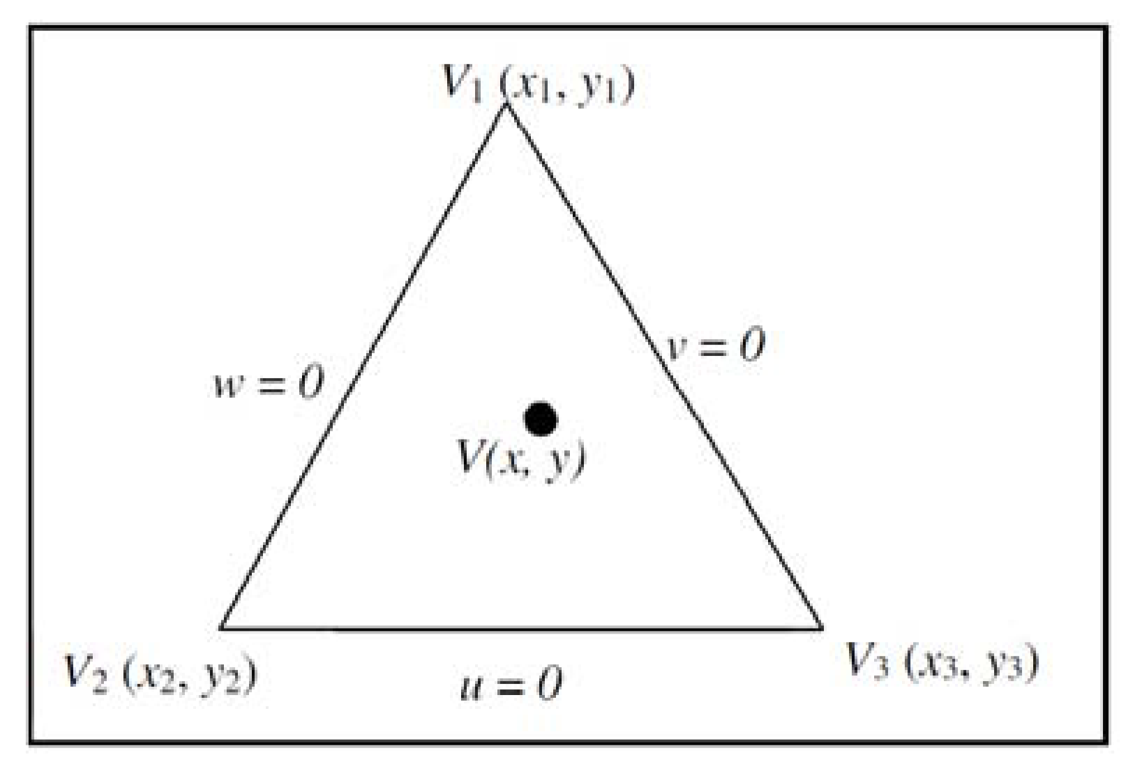
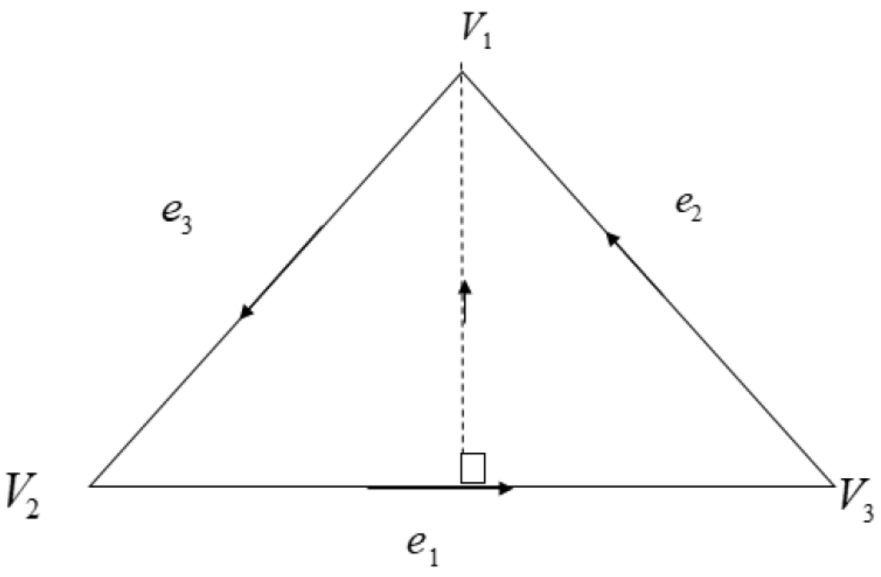
2.1. Review of the Cubic Triangular Bases of Zhu And Han

Zhu and Han [44] proposed a new cubic triangular basis with three exponential parameters $\alpha ,\beta ,\gamma .$ Since we are dealing with triangulation, the barycentric coordinate $\left(u,v,w\right)$ on the triangle $T_1$ with vertices $V_1,V_2$ and $V_3$ is defined by $u+v+w=1$, where $u,v,w\ge 0$. Set the point inside the triangle as $V\left(x,y\right)\in R^2$ (as shown in Figure 1), which can be expressed as:

$$V=u{V}_1+v{V}_2+w{V}_3$$

(1)

Definition 1. 

Let the parameters$\alpha ,\beta ,\gamma \in [2,\infty ]$and the triangular domain$D=\left\{\left(u,v,w\right)|u+v+w=1\right\}$; the following are cubic Bernstein–Bézier basis functions ([44]):

$$\begin{array}{cc}\hfill \left\{B_{3,0,0}^3\right(u,v,w;\alpha ,\beta ,\gamma )& =u^{\alpha }, B_{0,3,0}^3\left(u,v,w;\alpha ,\beta ,\gamma \right)=v^{\beta }, B_{0,0,3}^3\left(u,v,w;\alpha ,\beta ,\gamma \right)\hfill \\ & =w^{\gamma }, B_{2,1,0}^3\left(u,v,w;\alpha ,\beta ,\gamma \right)\hfill \\ & =u^{2}v \left[\frac{3-2u-u^{\alpha -2}}{1-u}\right], B_{2,0,1}^3\left(u,v,w;\alpha ,\beta ,\gamma \right)\hfill \\ & =u^{2}w \left[\frac{3-2u-u^{\alpha -2}}{1-u}\right], B_{1,2,0}^3\left(u,v,w;\alpha ,\beta ,\gamma \right)\hfill \\ & =u{v}^2 \left[\frac{3-2v-v^{\beta -2}}{1-v}\right], B_{0,2,1}^3\left(u,v,w;\alpha ,\beta ,\gamma \right)\hfill \\ & =v^{2}w \left[\frac{3-2v-v^{\beta -2}}{1-v}\right], B_{1,0,2}^3\left(u,v,w;\alpha ,\beta ,\gamma \right)\hfill \\ & =u{w}^2 \left[\frac{3-2w-w^{\gamma -2}}{1-w}\right], B_{0,1,2}^3\left(u,v,w;\alpha ,\beta ,\gamma \right)\hfill \\ & =v{w}^2 \left[\frac{3-2w-w^{\gamma -2}}{1-w}\right], B_{1,1,1}^3\left(u,v,w;\alpha ,\beta ,\gamma \right)=6uvw.\hfill \end{array}$$

(2)

Zhu and Han’s triangular basis functions satisfy the following properties:

Non-negativity:

$${\mathit{B}}_{\mathit{i},\mathit{j},\mathit{k}}^{\mathbf{3}}\left(\mathit{u},\mathit{v},\mathit{w};\mathit{\alpha },\mathit{\beta },\mathit{\gamma }\right)\ge \mathbf{0}, \mathit{i}+\mathit{j}+\mathit{k}=\mathbf{3}.$$

Partition of unity:

$${{\displaystyle \sum }}_{\mathit{i}+\mathit{j}+\mathit{k}=\mathbf{3}}{\mathit{B}}_{\mathit{i},\mathit{j},\mathit{k}}^{\mathbf{3}}\left(\mathit{u},\mathit{v},\mathit{w};\mathit{\alpha },\mathit{\beta },\mathit{\gamma }\right)=\mathbf{1}.$$

Symmetry:

$${\mathit{B}}_{\mathit{i},\mathit{j},\mathit{k}}^{\mathbf{3}}\left(\mathit{u},\mathit{v},\mathit{w};\mathit{\alpha },\mathit{\beta },\mathit{\gamma }\right)={\mathit{B}}_{\mathit{i}\mathit{j}\mathit{k}}^{\mathbf{3}}\left(\mathit{w},\mathit{v},\mathit{u};\mathit{\gamma },\mathit{\beta },\mathit{\alpha }\right).$$

For more details on the other properties, please refer to Zhu and Han [44].

Zhu and Han’s triangular patches with three parameters $\alpha ,\beta ,$ and $\gamma ,$ and control points $b_{ijk},i+j+k=3$ are defined as

$$P\left(u,v,w\right)={\displaystyle \sum }_{i+j+k=3}^{}{b}_{ijk}{B}_{i,j,k}^3\left(u,v,w;\alpha ,\beta ,\gamma \right), u+v+w=1$$

(3)

Figure 2 shows the Zhu and Han ordinates, and Figure 3 shows one patch of the Zhu and Han triangular with $\alpha =\beta =\gamma =3$ (i.e., cubic Bézier triangular).

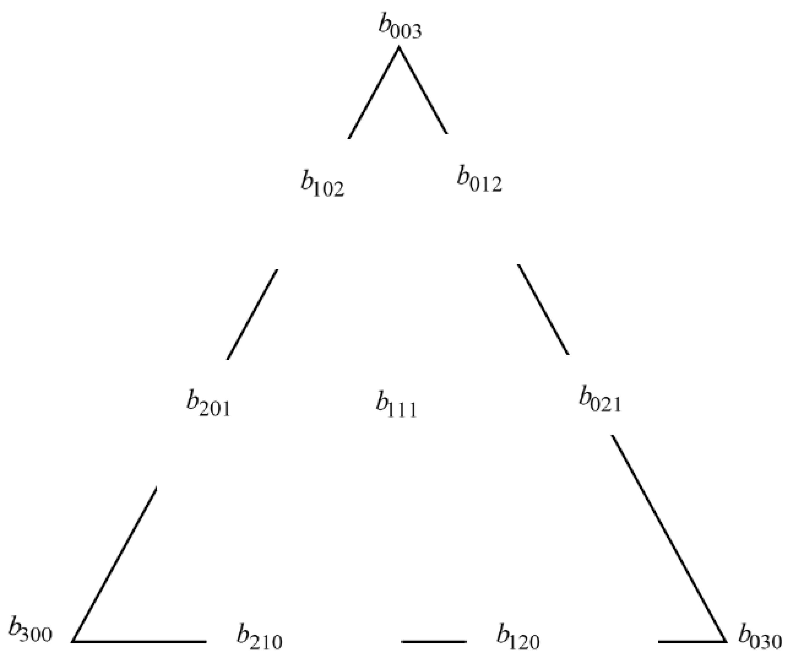
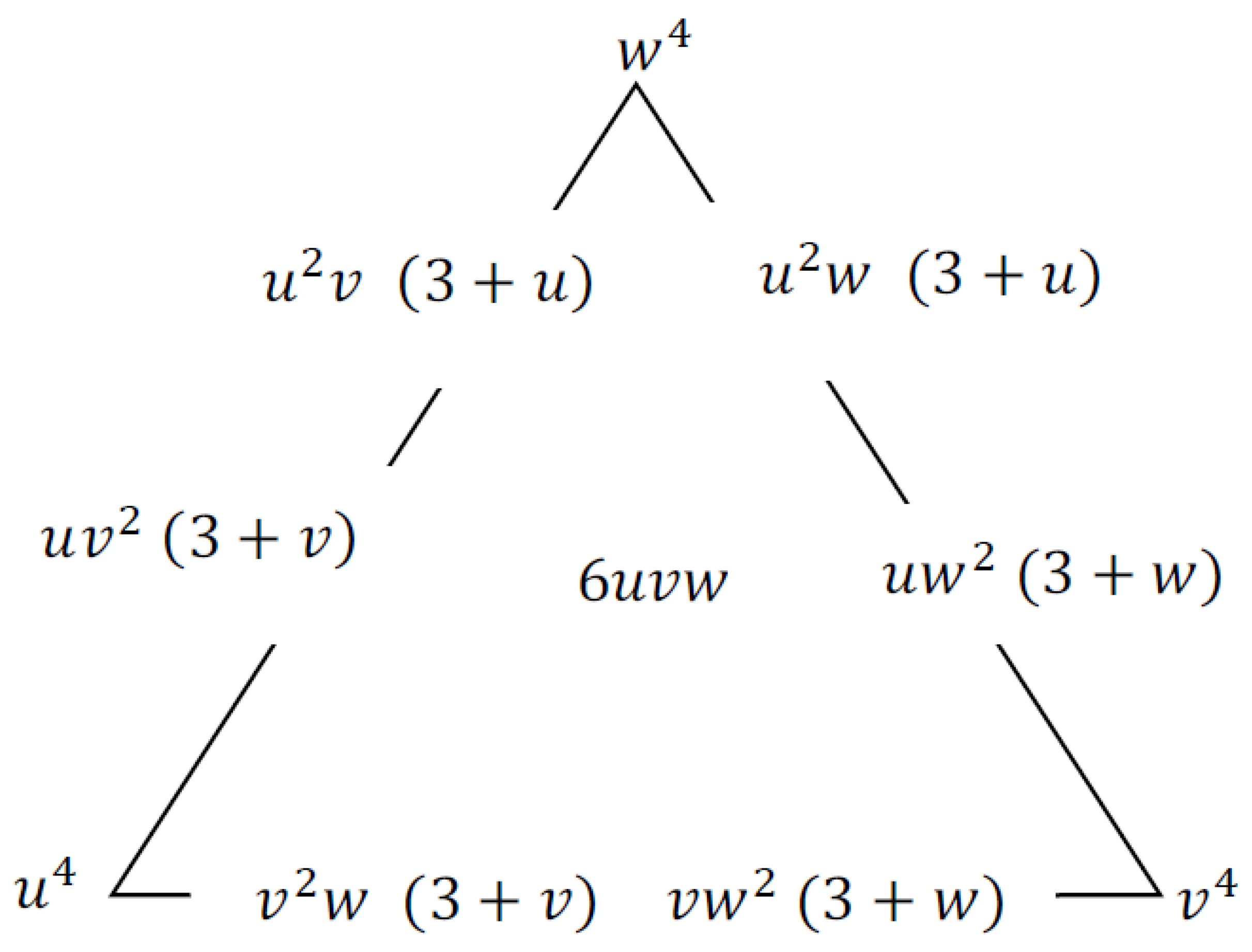
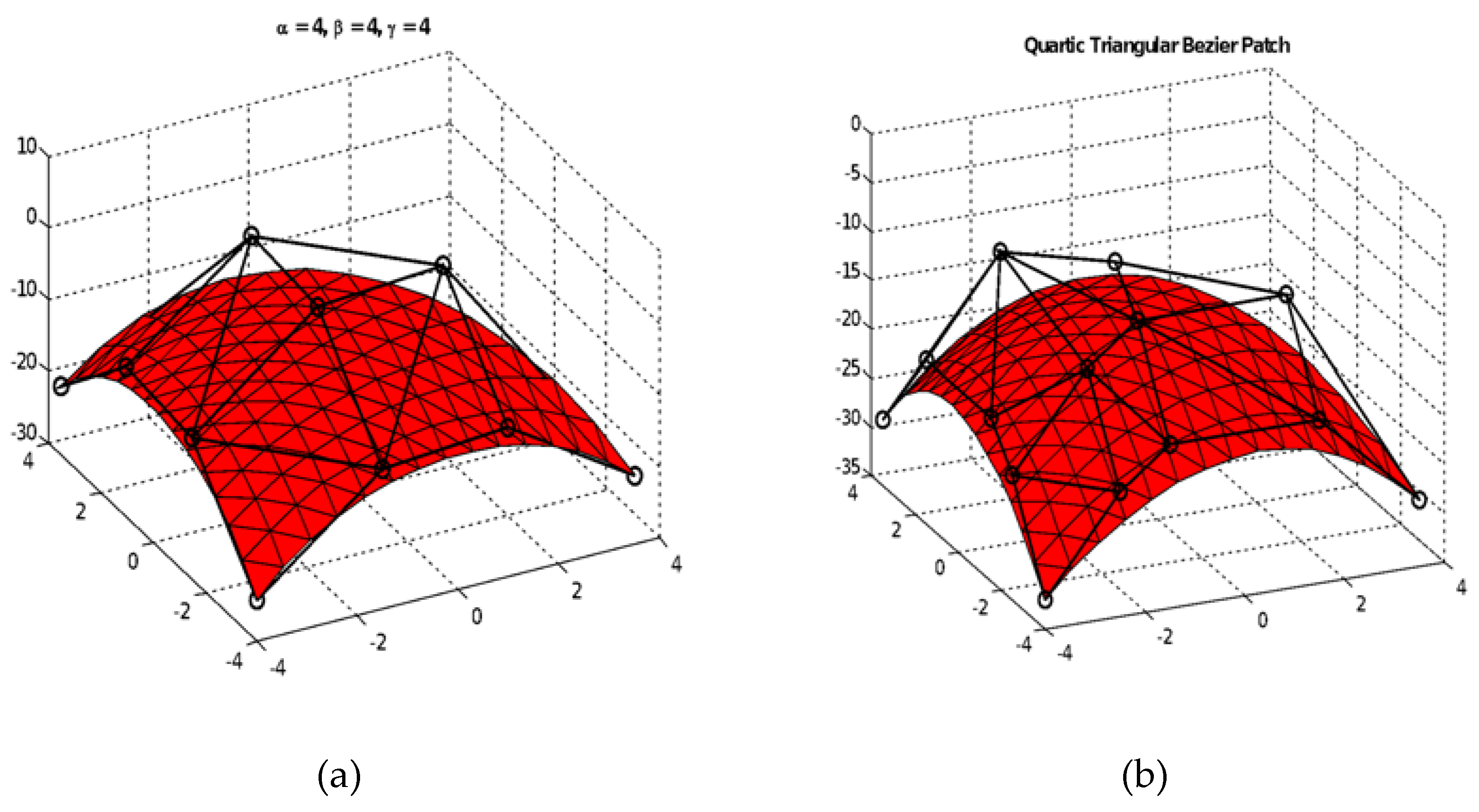
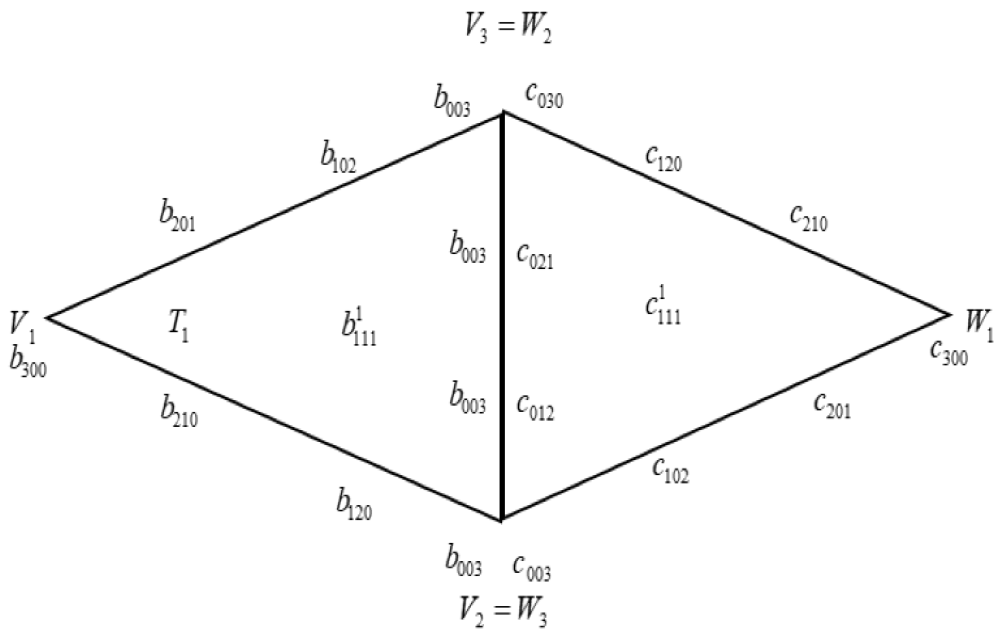
2.2. Quartic Zhu and Han Triangular Patches

From Equation (2), let $\alpha =\beta =\gamma =4$, then we obtain the following ten quartic basis functions defined on the triangular domain:

$$\begin{array}{cc}\hfill \left\{B_{3,0,0}^3\right(u,v,w;\alpha ,\beta ,\gamma )& =u^4, B_{0,3,0}^3\left(u,v,w;\alpha ,\beta ,\gamma \right)=v^4, B_{0,0,3}^3\left(u,v,w;\alpha ,\beta ,\gamma \right)\hfill \\ & =w^4, B_{2,1,0}^3\left(u,v,w;\alpha ,\beta ,\gamma \right)=u^{2}v \left(3+u\right), B_{2,0,1}^3\left(u,v,w;\alpha ,\beta ,\gamma \right)\hfill \\ & =u^{2}w \left(3+u\right), B_{1,2,0}^3\left(u,v,w;\alpha ,\beta ,\gamma \right)\hfill \\ & =u{v}^2 \left(3+v\right), B_{0,2,1}^3\left(u,v,w;\alpha ,\beta ,\gamma \right)\hfill \\ & =v^{2}w \left(3+v\right), B_{1,0,2}^3\left(u,v,w;\alpha ,\beta ,\gamma \right)\hfill \\ & =u{w}^2 \left(3+w\right), B_{0,1,2}^3\left(u,v,w;\alpha ,\beta ,\gamma \right)\hfill \\ & =v{w}^2 \left(3+w\right), B_{1,1,1}^3\left(u,v,w;\alpha ,\beta ,\gamma \right)=6uvw.\hfill \end{array}$$

(4)

Figure 4 shows the quartic triangular basis on the triangular domain.

Thus, the quartic Zhu and Han triangular patch can be defined by

$$\begin{array}{cc}\hfill P\left(u,v,w\right)& =u^4{b}_{300}+v^4{b}_{030}+w^4{b}_{003}+u^{2}v \left(3+u\right)b_{210}+\left(3+u\right)u^{2}w{b}_{201}\hfill \\ \hfill & +\left(3+v\right)v^{2}u{b}_{120}+\left(3+v\right)v^{2}w{b}_{021}+\left(3+w\right)w^{2}u{b}_{102}\hfill \\ \hfill & +\left(3+w\right)w^{2}v{b}_{012}+6uvw{b}_{111}\hfill \end{array}$$

(5)

The main advantage of Zhu and Han’s quartic is that it only requires ten control points to construct one triangular patch; meanwhile, the quartic Bézier triangular will require 15 control points to produce one patch. Furthermore, when the quartic Bézier triangular is used for scattered data interpolation, an optimization method is required to produce the interpolated surface, as discussed in Saaban et al. [35], Piah et al. [36] and Hussain et al. [37,38]. However, if we apply the proposed quartic triangular patches for scattered data interpolation, the optimization is not required since we can employ the cubic precision scheme of Foley and Opitz [30] to construct a $C^1$ interpolated surface everywhere. So far, this is the first study to apply a a quartic triangular basis but with ten control points for scattered data interpolation.

Figure 5a shows examples of quartic Zhu and Han, and Figure 5b shows the quartic Bézier triangular patch.

2.3. Scattered Data Interpolation Using Quartic Zhu and Han Triangular Patches

To apply the quartic triangular patch defined in Section 2.2 for scattered data, we use the local scheme comprising a convex combination between three local schemes $K_1,K_2$, and $K_3$ [1,9,24] such that:

$$\mathit{P}\left(\mathit{u},\mathit{v},\mathit{w}\right)=\frac{\mathit{v}\mathit{w}{\mathit{K}}_{\mathbf{1}}+\mathit{u}\mathit{w}{\mathit{K}}_{\mathbf{2}}+\mathit{u}\mathit{v}{\mathit{K}}_{\mathbf{3}}}{\mathit{v}\mathit{w}+\mathit{u}\mathit{w}+\mathit{u}\mathit{v}}, \mathit{u}+\mathit{v}+\mathit{w}=\mathbf{1}$$

(6)

The local scheme $K_i$, $i=1,2,3$ is obtained by replacing $b_{111}$ in (5) with $b_{111}^i$ to ensure the $C^1$ condition is satisfied. Given the vertex of the triangle (i.e., $F\left(V_1\right)=b_{300}, F\left(V_2\right)=b_{030},$ and $F\left(V_3\right)=b_{003}$), the derivative along $e_{jk}$ (see Figure 6)—that is, the edge connecting two points $\left(x_j-y_j\right)$ and $\left(x_k-y_k\right)$—is defined as [1,9,24,29]:

$$\frac{\partial P}{\partial e_{jk}}=\left(x_k-x_j\right)\frac{\partial F}{\partial x}+\left(y_k-y_j\right)\frac{\partial F}{\partial y}$$

Thus

$$b_{210}=F\left(V_1\right)+\frac{1}{4}\frac{\partial P}{\partial e_3}\left(V_1\right)$$

which can be simplified as

$$b_{210}=b_{300}+\frac{1}{4}\left(\left(x_2-x_1\right)F_x\left(V_1\right)+\left(y_2-y_1\right)F_y\left(V_1\right)\right)$$

(7)

Similarly, the other five ordinates are calculated as follows:

$$b_{201}=b_{300}-\frac{1}{4}\left(\left(x_1-x_3\right)F_x\left(V_1\right)+\left(y_1-y_3\right)F_y\left(V_1\right)\right)$$

(8)

$$b_{021}=b_{030}+\frac{1}{4}\left(\left(x_3-x_2\right)F_x\left(V_2\right)+\left(y_3-y_2\right)F_y\left(V_2\right)\right)$$

(9)

$$b_{120}=b_{030}-\frac{1}{4}\left(\left(x_2-x_1\right)F_x\left(V_2\right)+\left(y_2-y_1\right)F_y\left(V_2\right)\right)$$

(10)

$$b_{102}=b_{003}+\frac{1}{4}\left(\left(x_1-x_3\right)F_x\left(V_3\right)+\left(y_1-y_3\right)F_y\left(V_3\right)\right)$$

(11)

$$b_{012}=b_{003}-\frac{1}{4}\left(\left(x_3-x_2\right)F_x\left(V_3\right)+\left(y_3-y_2\right)F_y\left(V_3\right)\right)$$

(12)

The remaining $b_{111}^i$, $i=1,2,3$ is obtained by using the cubic precision of Foley and Opitz [30] as shown in Figure 7. For complete derivation, the reader can refer to [30].

In order to achieve C¹ continuity along all edges, the following equations must be satisfied:

$$c_{201}=r^2{b}_{210}+2st{b}_{021}+2rs{b}_{120}+s^2{b}_{030}+2rt{b}_{111}^2+t^2{b}_{012}$$

(13)

$$c_{210}=r^2{b}_{201}+2st{b}_{012}+2rt{b}_{102}+s^2{b}_{021}+2rs{b}_{111}^1+t^2{b}_{003}$$

(14)

$$b_{210}=u^2{c}_{201}+2vw{c}_{012}+2uw{c}_{102}+v^2{c}_{021}+2uv{c}_{111}^1+w^2{c}_{003}$$

(15)

$$b_{201}=u^2{c}_{210}+2vw{c}_{021}+2uw{c}_{120}+v^2{c}_{030}+2uv{c}_{111}^1+w^2{c}_{012}$$

(16)

To find $c_{111}^1$ in (13) and (14), we need to add these equations together. Thus, we obtain

$$\begin{array}{c}{c}_{111}^1=\frac{1}{2u\left(v+w\right)}\left(b_{201}+b_{210}-u^2\left(c_{210}+c_{201}\right)-v^2\left(c_{030}+c_{021}\right)\right)\\ \hspace{1em}\hspace{1em}\hspace{1em}\hspace{1em}\hspace{1em}+w^2\left(c_{012}+c_{003}\right)-2vw\left(c_{021}+c_{012}\right)-uv{c}_{120}-2uw{c}_{102}.\end{array}$$

Similarly, with Equations (15) and (16), we obtain

$$\begin{array}{c}{b}_{111}^1=\frac{1}{2r\left(s+t\right)}\left(c_{201}+c_{210}-r^2\left(b_{210}+b_{201}\right)-s^2\left(b_{030}+b_{021}\right)\right)\\ \hspace{1em}\hspace{1em}\hspace{1em}\hspace{1em}\hspace{1em}\hspace{1em}+t^2\left(b_{012}+b_{003}\right)-2st\left(b_{021}+b_{012}\right)-rs{b}_{120}-2rt{b}_{102}.\end{array}$$

Now we establish the theorem for the main result.

Theorem 1. 

The local scheme defined by (6) is a rational function with degree 7, that is, degree five in numerator and degree two in denominator with$C^1$continuity everywhere. It has the following form:

$$P\left(u,v,w\right)={\displaystyle \sum }_{i+j+k=3 i,j,k\ne 1 }^{}{b}_{ijk}{B}_{i,j,k}^3\left(u,v,w\right)+6uvw \left(a_1{b}_{111}^1+a_2{b}_{111}^2+a_3{b}_{111}^3\right)$$

(17)

with

$$a_1=\frac{vw}{vw+uw+uv},a_2=\frac{uw}{vw+uw+uv},a_3=\frac{uv}{vw+uw+uv}$$

(18)

and the barycentric coordinate satisfies$u+v+w=1$.

The following Algorithm 1 can be used to implement the proposed scheme.

Algorithm 1 (Scattered Data Interpolation)

Step 1: Input scattered data points; Step 2: Estimate the partial derivative at the data points by using [25]; Step 3: Triangulate the domain of the data points; Step 4: Calculate the boundary control points using Equations (7)–(12); Step 5: Calculate inner control points for the local scheme, $b_{111}^i$, $i=1,2,3$ by using the cubic precision method as in Foley and Opitz [30]; Step 6: Construct the interpolated surface using the convex combination method of three local schemes defined by (6); Step 7: Calculate CPU time (in seconds), R2, and maximum error. Repeat steps 1 through 6 for the other scattered data sets.

Below we give the theorem for scattered data interpolation by using quartic Bézier triangular patches.

Theorem 2. 

C¹ quartic Bézier triangular patches using minimized sum of squares of principal curvatures [35].

Let the quartic Bézier triangular patch (n = 4) with barycentric coordinates u, v, w be expressed as

$$S\left(u, v, w\right)={\displaystyle \sum }_{i+j+k=4}^{}{c}_{ijk}{B}_{ijk}^4\left(u,v,w\right)$$

(19)

where $B_{ijk}^4\left(u,v,w\right)=\frac{4!}{i!j!k!}{u}^i{v}^j{v}^k$ and $c_{ijk}$ are the Bézier ordinates of S. Let the total number of triangles in the whole triangular mesh be n_t and the total number of interior edges be n_e. S(x,y) which will minimize the functional I(S(x,y)) leads to the optimization problem x^T Qx + ex + h, subject to the C¹ continuity constraint:

$$min{ }_x{x}^{T}Qx+ex+h\mathrm{subject}\mathrm{to}\mathrm{Ax}=\mathbf{b}$$

(20)

where Q is a 6n_t × 6n_t sparse matrix, e is a 1 × 6n_t row vector, x is a 6n_t × 1 column vector consisting of unknown ordinates $\left(b_{220}^m b_{211}^m b_{121}^m b_{202}^m b_{112}^m b_{022}^m\right),m=1,\dots ,n_t$, h is a real constant, A is a 3n_e × 6n_t ($3n_e\le 6n_t$) coefficient matrix, x is a 6n_t × 1 unknown column vector consisting of the remaining ordinates b₂₂₀, b₂₀₂, b₀₂₂, b₂₁₁, b₁₂₁ and b₁₁₂ to be determined for the entire triangular mesh, and b is a 3n_e × 1 constant column vector. The optimization problem stated in (18) was solved using the optimization toolbox in MATLAB 2017 on Intel^® Core ™ i5-8250U 1.60 GHz.

Note that the optimization problem in Theorem 2 is obtained by using a minimized principal curvature norm with respect to the C¹ continuity constraint, which results in a global method for scattered data interpolation. Meanwhile, by using the proposed scheme in this study, the resulting surface is local.

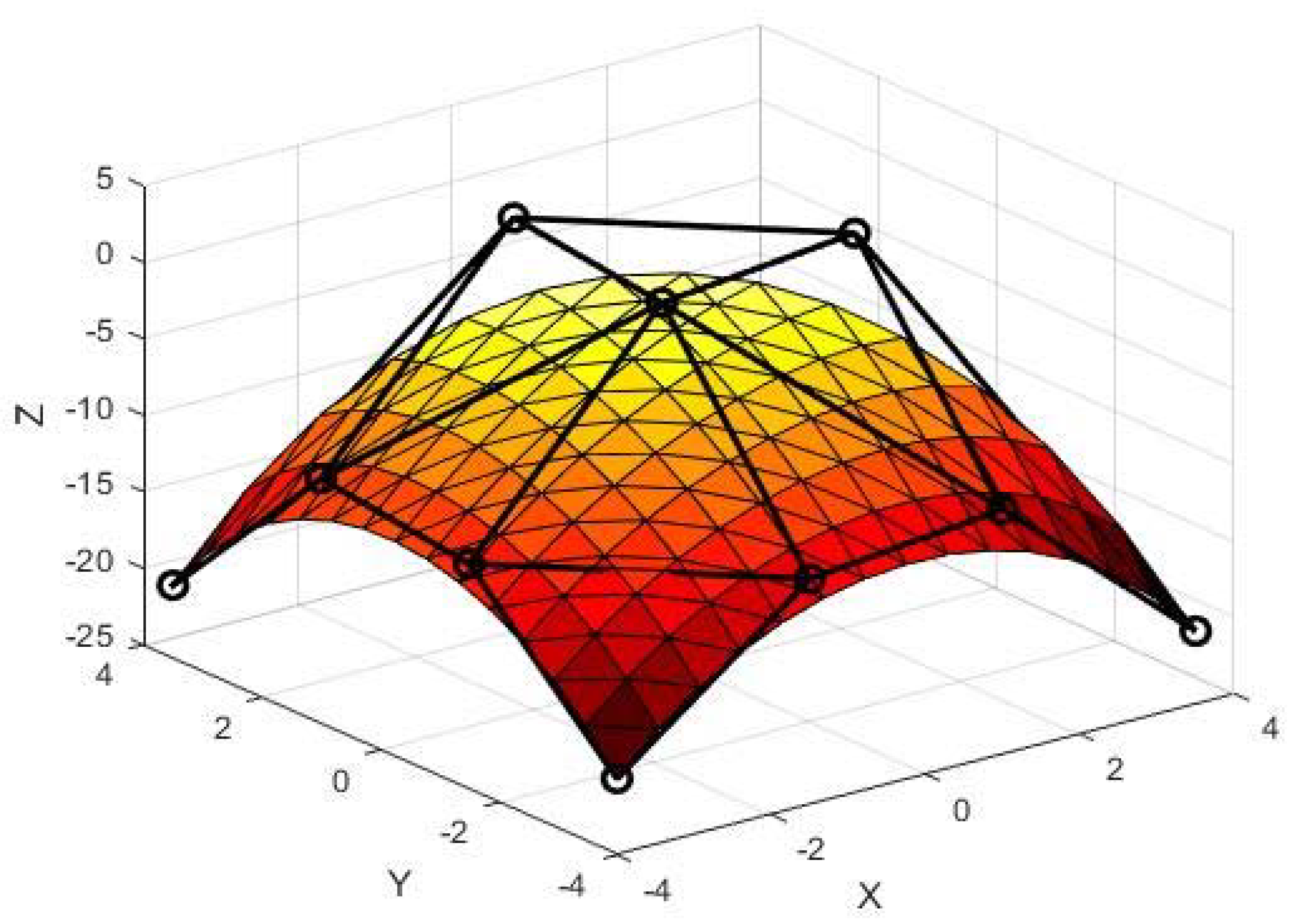
3. Results and Discussion for Scattered Data Interpolation

We tested the proposed scheme using two well-known test functions $F_1\left(x,y\right)$ and $F_2\left(x,y\right)$:

$$\begin{array}{c}{F}_1\left(x,y\right)=0.75e^{\left(-{\left(9x-2\right)}^2+{\left(9y-2\right)}^2/4\right)}+0.75e^{\left(-{\left(9x+1\right)}^2/49-{\left(9y+1\right)}^2/10\right)}\\ +0.5e^{\left(-{\left(9x-7\right)}^2+{\left(9y-3\right)}^2/4\right)}-0.2e^{\left(-{\left(9x-4\right)}^2-{\left(9y-7\right)}^2\right)}\end{array}$$

(21)

$$F_2\left(x,y\right)=\frac{\left(1.25+coscos \left(5.4y\right)\right)}{6+6{\left(3x-1\right)}^2}$$

(22)

We implemented the proposed scheme using MATLAB 2017 version on Intel^® Core ™ i5-8250U 1.60 GHz. MATLAB coding was developed based on Algorithm 1. About 25 MATLAB functions were used to obtain all the results.

We chose 36 data point samples in the domain $\left[0,1\right]\times \left[0,1\right],$ as shown in

Table 1. Data points.

x	y	F1(x,y)	F2(x,y)	x	y	F1(x,y)	F2(x,y)
0	0	0.7664	1.3333	0.80	0.85	0.0823	1.2431
0.50	0	0.4349	1.3833	0.85	0.65	0.1412	1.2043
1.00	0	0.1076	1.2833	1.00	0.50	0.1610	1.2199
0.15	0.15	1.1370	1.3382	1.00	1.00	0.0359	1.2712
0.70	0.15	0.4304	1.3020	0.50	1.00	0.1460	1.3346
0.50	0.20	0.5345	1.3128	0.10	0.85	0.2935	1.2363
0.25	0.30	1.0726	1.2423	0	1.00	0.2703	1.3029
0.40	0.30	0.7134	1.2421	0.25	0	0.8189	1.4069
0.75	0.40	0.5903	1.2139	0.75	0	0.2521	1.3150
0.85	0.25	0.5088	1.2607	0.25	1.00	0.2222	1.3496
0.55	0.45	0.3823	1.1613	0	0.25	0.8026	1.2683
0	0.50	0.4818	1.1747	0.75	1.00	0.0810	1.2913
0.20	0.45	0.6458	1.1412	0	0.75	0.3395	1.1987
0.45	0.55	0.2946	1.1037	1.00	0.25	0.2302	1.2573
0.60	0.65	0.1920	1.1552	1.00	0.75	0.0504	1.2295
0.25	0.70	0.2930	1.1240	0.19	0.19	1.2118	1.3229
0.40	0.80	0.0515	1.1887	0.32	0.75	0.2029	1.1477
0.65	0.75	0.1372	1.1961	0.79	0.46	0.4777	1.2041

. Figure 8 shows the Delaunay triangulation for the data. Figure 6 shows examples of surface interpolation for both functions. Comparing Figure 9 and Figure 10, the surfaces produced by the proposed scheme visually look smoother than the surfaces obtained from the quartic Bézier triangular of Saaban et al. [35] and Piah et al. [36]. Figure 10 shows an example of scattered data interpolation using quartic Bézier triangular patches.

To validate the proposed scheme, we calculated the maximum error (Max Error) and coefficient of determination (COD; i.e., R²) for both functions and compared them with those obtained for quartic Bézier triangular for three different numbers of points i.e., 100, 65, and 36 for both functions $F_1\left(x,y\right)$ and $F_2\left(x,y\right)$. Functions 1 and 2 represent $F_1\left(x,y\right)$ and $F_2\left(x,y\right)$, respectively.

Table 2. Error analysis.

Num. of Data Points	Function	Max Error		R2
		The Proposed Scheme	Quartic Bézier [35]	The Proposed Scheme	Quartic Bézier [35]
100	1	3.436 × 10∧−2	3.598 × 10∧−2	0.99936	0.99934
	2	4.500 × 10∧−2	7.61 × 10∧−2	0.99977	0.99967
65	1	6.410 × 10∧−2	6.586 × 10∧−2	0.99720	0.99733
	2	1.732 × 10∧−2	1.562 × 10∧−2	0.99796	0.99793
36	1	9.740 × 10∧−2	9.973 × 10∧−2	0.99211	0.99256
	2	2.675 × 10∧−2	2.762 × 10∧−2	0.99332	0.99208

shows the error analysis for both tested functions by using (a) quartic Zhu and Han and (b) quartic Bézier triangular. Meanwhile,

Table 3. CPU time (in seconds).

Num. of Data Points	Function	CPU Time (in Seconds)
		The Proposed Scheme	Quartic Bézier [35]
100	1	0.7097807844	5.6002481345
	2	0.4234289196	3.5703151686
65	1	0.2741610887	1.5474957467
	2	0.2363209917	1.3271791002
36	1	0.1298699059	0.5886074910
	2	0.1163838547	0.4703613961

shows CPU time in seconds. From Table 2, we can see that the proposed quartic triangular patches for scattered data interpolation gave smaller Max Error values than the quartic Bézier triangular. Additionally, the proposed scheme gave higher R² values for all numbers of data points (100, 65, and 36). From Table 3, the proposed scheme required less CPU time than the quartic Bézier. For instance, for 100 data points, the proposed scheme only required 0.71 s for data from function $F_1\left(x,y\right)$ and 0.42 s for data from function $F_2\left(x,y\right),$ compared with the quartic Bézier which requires 5.6 s and 3.57 s for 100 data points from functions $F_1\left(x,y\right)$ and $F_2\left(x,y\right)$, respectively. Thus, the proposed scheme in this study gave very good results, and was better at treating scattered data than using the quartic Bézier triangular proposed by Piah et al. [36], Saaban et al. [35], and Hussain et al. [37,38]. We conclude that the proposed scheme required less CPU time than the quartic Bézier triangular. This reduction of CPU time consumption is an advantage when the goal is to construct a surface with thousands of data points or big data.

This can be seen clearly from Table 3. With the largest number of data points, the CPU time for the proposed scheme was approximately 12.5% that of the CPU time required for the quartic Bézier triangular based scheme. This is very significant, especially when the user wants to render and reconstruct surfaces obtained from very dense data sets. Many studies in scattered data interpolation usually involve the use of Shepard-type interpolants such as Shepard triangular schemes for scattered data interpolation [6,11,12,13]. We also implemented the Shepard triangular to the same data sets as listed in Table 1.

Table 4. Error analysis.

Num. of Data Points	Function	Max Err
		Dell’Accio et al. [12]	Dell’Accio and Di Tommaso [11]	Dell’Accio et al., [12] and Cavoretto et al. [6]	Dell’Accio et al. [12]	Dell’Accio et al. [13] and Cavoretto et al. [6]
100	1	5.2990 × 10∧−2	8.6648 × 10∧−2	1.0970 × 10∧−1	6.2438 × 10∧−2	5.3936 × 10∧2
	2	1.8617 × 10∧−2	5.0590 × 10∧−2	3.2842 × 10∧−2	1.5449 × 10∧−2	1.9619 × 10∧−2
65	1	1.0147 × 10∧−1	1.1864 × 10∧−1	1.1221 × 10∧−1	7.6266 × 10∧−2	7.1704 × 10∧−2
	2	6.4329 × 10∧−2	3.7704 × 10∧−2	3.5962 × 10∧−2	2.7322 × 10∧−2	2.8894 × 10∧−2
36	1	1.2822 × 10∧−1	1.6219 × 10∧−1	1.3564 × 10∧−1	1.1371 × 10∧−1	9.8914 × 10∧−2
	2	7.9686 × 10∧−2	5.6713 × 10∧−2	5.3611 × 10∧−2	5.1806 × 10∧−2	4.6253×10∧−2

and

Table 5. CPU time (in seconds).

Num. of Data Points	Function	CPU Time (Second)
		Dell’Accio et al. [12]	Dell’Accio and Di Tommaso [11]	Dell’Accio et al., [12] and Cavoretto et al. [6]	Dell’Accio et al. [12]	Dell’Accio et al. [13] and Cavoretto et al. [6]
100	1	0.490380	1.894685	0.480296	0.423177	0.401825
	2	0.502923	1.881019	0.501286	0.428949	0.417658
65	1	0.486381	1.882420	0.478175	0.424583	0.424086
	2	0.484984	1.849458	0.459517	0.424870	0.397832
36	1	0.437090	1.707668	0.445523	0.415162	0.445566
	2	0.448242	1.686242	0.448589	0.417875	0.421869

show the error analysis for the schemes of Cavoretto et al. [6], Dell’Accio et al. [12,13], and Dell’Accio and Di Tommaso [11]. Based on CPU time, for all tested data sets, the proposed scheme was faster than the schemes in [6,11,12,13], except for the case with 100 data points for the data from function $F_1\left(x,y\right).$ Considering the Max Error, the proposed scheme was better than all four schemes except for the case with 100 data points from function $F_2\left(x,y\right).$ Therefore, we can conclude that the proposed scheme is better than quartic triangular patch and the Shepard triangular based schemes [6,11,12,13].

4. Positivity-Preserving Scattered Data Interpolation

In this section, we apply the proposed scheme discussed in the previous section to preserve the positivity of scattered data sets. To do this, first we derive the sufficient condition for the positivity of the quartic triangular spline defined in (5). Finally, the rational corrected scheme defined by (19) will be used to construct a positive surface with C¹ continuity.

To derive the sufficient condition for the positivity of the quartic spline triangular patch, we adopted a similar approach to Saaban et al. [35] and Piah et al. [36]. Assume that the quartic ordinates at the vertices are strictly positive such $b_{300},b_{030},b_{003}>0$. Let $A=b_{300},B=b_{030},C=b_{003},$ therefore $A,B,C>0$ (see Figure 11). Meanwhile, let the other ordinates have the same value, that is $-t<0$ where $t>0$. Thus, Equation (5) becomes

$$\begin{array}{cc}\hfill P\left(u,v,w\right)=A{u}^4& +B{v}^4+C{w}^4\hfill \\ & -t(u^{2}v \left(3+u\right)+\left(3+u\right)u^{2}w+\left(3+v\right)v^{2}u+\left(3+v\right)v^{2}w+\left(3+w\right)w^{2}u\hfill \\ & +\left(3+w\right)w^{2}v+6uvw)\hfill \\ & =A{u}^4+B{v}^4+C{w}^4-t\left(1-u^4-v^4-w^4\right)\hfill \\ & =\left(A+t\right)u^4+\left(B+t\right)v^4+\left(C+t\right)w^4-t\hfill \end{array}$$

(23)

From (23) we can observe that when $t=0$ then $P\left(u,v,w\right)>0$. Meanwhile as $t$ increases, $P\left(u,v,w\right)$ decreases. We want to find the value of $t=t_0$ when the minimum value of $P\left(u,v,w\right)=0$. By taking first partial derivatives, we will obtain the following:

$$\begin{gathered} \frac{\partial P\left(u,v,w\right)}{\partial u}=4\left(A+t\right)u^3, \\ \frac{\partial P\left(u,v,w\right)}{\partial v}=4\left(B+t\right)v^3, \\ \frac{\partial P\left(u,v,w\right)}{\partial w}=4\left(C+t\right)w^3. \end{gathered}$$

(24)

The minimum value of $P\left(u,v,w\right)$ occurs when

$\frac{\partial P}{\partial u}-\frac{\partial P}{\partial v}=0$ and $\frac{\partial P}{\partial u}-\frac{\partial P}{\partial w}=0$ or equivalently.

$$\frac{\partial P}{\partial u}=\frac{\partial P}{\partial v}=\frac{\partial P}{\partial w}$$

(25)

From Equation (25) we have

$\frac{u^3}{v^3}=\frac{B+t}{A+t}$ and $\frac{u^3}{w^3}=\frac{C+t}{A+t}$

Hence:

$$u^3:v^3:w^3=\frac{1}{A+t}:\frac{1}{B+t}:\frac{1}{C+t}.$$

Since $u+v+w=1$, we obtain the following relations:

$$u=\frac{\frac{1}{{\left(A+t\right)}^{1/3}}}{\frac{1}{{\left(A+t\right)}^{1/3}}+\frac{1}{{\left(B+t\right)}^{1/3}}+\frac{1}{{\left(C+t\right)}^{1/3}}},$$

$$v=\frac{\frac{1}{{\left(B+t\right)}^{1/3}}}{\frac{1}{{\left(A+t\right)}^{1/3}}+\frac{1}{{\left(B+t\right)}^{1/3}}+\frac{1}{{\left(C+t\right)}^{1/3}}}, \mathrm{and}$$

$$w=\frac{\frac{1}{{\left(C+t\right)}^{1/3}}}{\frac{1}{{\left(A+t\right)}^{1/3}}+\frac{1}{{\left(B+t\right)}^{1/3}}+\frac{1}{{\left(C+t\right)}^{1/3}}}.$$

Substituting this value into (23) we obtain the minimum value of $P\left(u,v,w\right)$ i.e.,

$P\left(u,v,w\right){\frac{1}{{\left[\frac{1}{{\left(A+t\right)}^{1/3}}+\frac{1}{{\left(B+t\right)}^{1/3}}+\frac{1}{{\left(C+t\right)}^{1/3}}\right]}^3}}_{min}$ which can be simplified to

$$P\left(u,v,w\right){\frac{t}{{\left[\frac{1}{{\left(A/t+1\right)}^{1/3}}+\frac{1}{{\left(B/t+1\right)}^{1/3}}+\frac{1}{{\left(C/t+1\right)}^{1/3}}\right]}^3}}_{min}$$

(26)

Now, $P{\left(u,v,w\right)}_{min}$ when

$$\frac{1}{{\left(A/t+1\right)}^{1/3}}+\frac{1}{{\left(B/t+1\right)}^{1/3}}+\frac{1}{{\left(C/t+1\right)}^{1/3}}=1$$

(27)

Let $s=1/t$, then

$$G\left(s\right)=\frac{1}{{\left(As+1\right)}^{1/3}}+\frac{1}{{\left(Bs+1\right)}^{1/3}}+\frac{1}{{\left(Cs+1\right)}^{1/3}}$$

(28)

Then Equation (27) can be written as $G\left(s\right)=1,s\ge 0$. This equation can be solved by using regula-falsi method with suitable choice of initial guess.

Since $A,B,C>0$ and $s\ge 0$ then $G^{\prime }\left(s\right)<0$ and $G^{″}\left(s\right)>0.$ (see Figure 12). Thus, the curve is convex on that region. Let $X=\mathit{max}\left(A,B,C\right)$ and $Y=\mathit{min}\left(A,B,C\right)$, then the following holds

$$\frac{3}{\sqrt[3]{Xs+1}}\le G\left(s\right)\le \frac{3}{\sqrt[3]{Ys+1}}$$

Such that

$$G\left(\frac{26}{X}\right)\ge 1 \mathrm{and}G\left(\frac{26}{Y}\right)\le 1.$$

Figure 12 shows the example of the relative locations of $\frac{26}{X}$ and $\frac{26}{Y}$ and $s_0$.

Now we establish the main theorem for positivity preservation using the proposed scheme.

Theorem 3. 

Consider the quartic triangular patch$P\left(u,v,w\right)$with vertex$A=b_{300},B=b_{030},C=b_{003},$such that$A,B,C>0$. If the remaining quartic triangular ordinates are equal to$-t_0$where$t_0=\frac{1}{s_0}$is a unique solution to (28), then$P\left(u,v,w\right)\ge 0$for all$u,v,w\ge 0$and$u+v+w=1$.

Some observations from Theorem 3 can be made as follows:

Let $A=B>C=1$. Then, we have

$$G\left(s\right)=\frac{2}{{\left(As+1\right)}^{1/3}}+\frac{1}{{\left(s+1\right)}^{1/3}}$$

Therefore, as $A\to \infty$, then $G\left(s\right)\to \frac{1}{{\left(s+1\right)}^{1/3}}$. Hence, $s_0\to 0$ and therefore $t_0\to \infty$. Thus, the ordinate values are unbounded compared with the work of Chan and Ong [7] in which the Bézier ordinates are bounded by a lower bound −1/3.

Remark 1. 

The sufficient condition for the positivity of the quartic triangular patch developed in this study is the same as the sufficient condition for the quartic Bézier triangular patch developed in Saaban et al. [35]. The main difference is that the proposed quartic polynomial only requires ten control points (or ordinates) as compared to the quartic Bézier triangular which requires 15 control points and involves some optimization problems as shown in Saaban et al. [35] and Hussain et al. [37,38]. Therefore, the proposed positivity preservation using a quartic triangular patch requires less computation time than some established schemes for scattered data interpolation.

The final construction of the positive scattered surface is described below:

1. Input positive scattered data points;

2. Triangulate the scattered data using Delaunay triangulation;

3. Assign the first partial derivative at the respective data sites and adjust if necessary, to provide the positivity preservation;

4. The $C^1$ triangular surface is constructed via convex combination between three local schemes;

5. Repeat Steps 1 through 4 for other positive scattered data sets.

5. Numerical Results and Discussion for Positivity-Preserving Scattered Data Interpolation

After we derive the sufficient condition for the positivity of quartic triangular patch, the final $C^1$ scattered data scheme for positivity preservation can be written as follows:

$$P\left(u,v,w\right)={\displaystyle \sum }_{\begin{array}{c}i+j+k=3\\ i,j,k\ne 1\end{array}}{b}_{ijk}{B}_{i,j,k}^3\left(u,v,w\right)+6uvw\left(a_1{b}_{111}^1+a_2{b}_{111}^2+a_3{b}_{111}^3\right)$$

(29)

with

$$a_1=\frac{vw}{vw+uw+uv},a_2=\frac{uw}{vw+uw+uv},a_3=\frac{uv}{vw+uw+uv}$$

(30)

We test the proposed scheme by using four well-known test functions given below:

$$F_1\left(x,y\right)=\{\begin{array}{c}1.0\mathrm{if}\left(y-x\right)\ge 0.5\hfill \\ 2\left(y-x\right)\mathrm{if}0.5\ge \left(y-x\right)\ge 0.0\hfill \\ \frac{\mathit{cos}(4\pi \sqrt{{(x-1.5)}^2+{(y-0.5)}^2}+1}{2}\mathrm{if}{(x-1.5)}^2+{(y-0.5)}^2\le \frac{1}{16}\hfill \\ 0\mathrm{elsewhereon}\left[0,2\left]x\right[0,1\right]\hfill \end{array}$$

$$\begin{array}{l}{F}_2\left(x,y\right)=1.025-0.75e^{-{(6x-1)}^2-{(6y-1)}^2⥂⥂}-0.75e^{-{(9x+1)}^2/49-{(9y+1)}^2/10}\\ -0.5e^{-{(9x-7)}^2-{(9y-3)}^2}-0.5e^{-{(10x-4)}^2-{(10y-7)}^2}\end{array}$$

$$F_3\left(x,y\right)=x^4+y^4$$

$$F_4\left(x,y\right)=e^{-{(5-10x)}^2/2}+0.75e^{-{(5-10y)}^2/2}+0.75e^{-{(5-10x)}^2/2}{e}^{-{(5-10y)}^2/2}$$

The positive test functions F₁, F₂, F₃, and F₄ were evaluated on 36, 33, 26, and 100 node points respectively (

Table 6. Value of F₁ on 36 node points.

x	y	F1(x,y)	x	y	F1(x,y)	x	y	F1(x,y)
0	0	0	0.35	0	0	1.4	0.8	0
0.2	0.2	0	0.8	0	0	1.65	0.75	0
0.5	0.2	0	0.1	0.85	1	2	1	0
0.4	0.4	0	0	0.25	0.5	1.25	0	0
0.75	0.35	0	0.8	1	0.4	1.7	0	0
0	0.5	1	2	0	0	1.25	1	0
0.25	0.5	0.5	1.4	0.3	0.0272	1.7	1	0
0.25	0.75	1	1.75	0.45	0	2	0.35	0
0.55	0.75	0.4	1.2	0.45	0	2	0.7	0
0.7	0.6	0	1.45	0.5	0.9045	1.05	0.2	0
0.5	1	1	1.6	0.3	0.0272	1	0.5	0
0	1	1	1.25	0.7	0	0.95	0.8	0

,

Table 7. Value of F₂ on 33 node points.

x	y	F2(x,y)	x	y	F2(x,y)	x	y	F2(x,y)
0	0	0.2586	0	0.50	0.5960	0.50	1.00	0.8762
0.50	0	0.6429	0.25	0.45	0.6264	0.10	0.85	0.7316
1.00	0	0.9174	0.45	0.55	0.7981	0	1.00	0.7547
0.25	0.20	0.0056	0.60	0.65	0.8336	0.25	0	0.2629
0.70	0.15	0.6012	0.25	0.70	0.7862	0.75	0	0.7739
0.50	0.20	0.6329	0.40	0.80	0.9941	0.25	1.00	0.8026
0.30	0.30	0.4199	0.65	0.75	0.8825	0	0.25	0.2792
0.45	0.35	0.6618	0.80	0.85	0.9427	0.75	1.00	0.9440
0.75	0.40	0.4361	0.85	0.65	0.8838	0	0.75	0.6865
0.85	0.25	0.5164	1.00	0.50	0.8640	1.00	0.25	0.7948
0.55	0.45	0.6724	1.00	1.00	0.9891	1.00	0.75	0.9746

,

Table 8. Value of F₃ on 26 node points.

x	y	F3(x,y)	x	y	F3(x,y)	x	y	F3(x,y)
0.9375	−0.4063	0.7997	0.0469	−0.7656	0.3436	−0.5156	−0.1094	0.0708
−0.1719	1.0000	1.0009	−0.7813	−0.8906	1.0017	0.4844	0.1406	0.0554
−0.8906	−0.0938	0.6292	0.0625	0.3750	0.0198	−0.4531	0.1563	0.0427
−0.0625	−0.6719	0.2038	−0.7656	−0.2969	0.3513	0.7031	0.3281	0.2560
−0.8750	−0.6250	0.7388	0.0938	0.1250	0.0003	−0.4219	0.4688	0.0800
0	0.7969	0.4033	−0.6875	0.3750	0.2432	0.9063	−0.5938	0.7990
−0.8438	−0.5313	0.5866	0.1094	0.3281	0.0117	−0.2344	0.1406	0.0034
0.0313	0.5313	0.0797	−0.5625	−0.6563	0.2856	0.9688	0.7188	1.1476
−0.8438	0.1563	0.5075	0.1563	0.4531	0.0427

and

Table 9. Value of F₄ on 100 node points.

x	y	F4 (x,y)	x	y	F4 (x,y)	x	y	F4 (x,y)
0.0096	0.3083	0.119425	0.3307	0.5159	1.155816	0.6677	0.6764	0.442125
0.0216	0.245	0.029055	0.3379	0.9426	0.268844	0.6814	0.8444	0.195332
0.0298	0.8614	0.00111	0.3439	0.48	1.248258	0.6888	0.3273	0.365476
0.0417	0.0978	0.000258	0.353	0.1783	0.345127	0.6941	0.1894	0.158965
0.047	0.3648	0.300748	0.3636	0.1147	0.395081	0.7062	0.0646	0.119387
0.0563	0.7156	0.073456	0.3766	0.8226	0.473071	0.7161	0.018	0.096822
0.0647	0.5311	0.714724	0.3822	0.2271	0.526808	0.7317	0.8905	0.068664
0.074	0.9756	0.000124	0.387	0.4074	1.274589	0.7371	0.4161	0.619367
0.0874	0.1781	0.004419	0.3973	0.8875	0.590813	0.7462	0.4689	0.797375
0.0935	0.5453	0.677296	0.4171	0.7632	0.749339	0.7567	0.2175	0.051462
0.1032	0.1604	0.00273	0.4256	0.9973	0.758236	0.77	0.5734	0.613977
0.111	0.7837	0.013932	0.4299	0.496	2.117705	0.7879	0.8853	0.016309
0.1181	0.9982	0.000684	0.4373	0.341	1.207499	0.7944	0.8018	0.021117
0.1252	0.6911	0.121795	0.4705	0.2498	1.021601	0.8164	0.6389	0.294451
0.1327	0.105	0.001483	0.4737	0.6409	1.512454	0.8193	0.8931	0.006444
0.144	0.8185	0.00648	0.4879	0.1059	0.99334	0.8368	0.1001	0.003695
0.1565	0.7086	0.088121	0.494	0.5412	2.374907	0.8501	0.279	0.067559
0.1651	0.4457	0.653239	0.5055	0.009	0.998497	0.8588	0.9083	0.001782
0.1786	0.1178	0.006221	0.5163	0.8784	0.987962	0.8646	0.3259	0.166279
0.1886	0.3189	0.154486	0.5219	0.5516	2.273778	0.8792	0.8319	0.003798
0.2017	0.9668	0.011703	0.5349	0.4039	1.858252	0.8838	0.0509	0.000664
0.21	0.7572	0.042784	0.5483	0.1654	0.895154	0.89	0.9708	0.000509
0.2147	0.2017	0.025997	0.557	0.2965	1.02504	0.897	0.5121	0.745189
0.2204	0.3232	0.180361	0.5639	0.366	1.370095	0.9045	0.286	0.076266
0.2344	0.4369	0.662063	0.5785	0.0367	0.734861	0.9084	0.9582	0.00026
0.241	0.8908	0.035317	0.5864	0.9502	0.688545	0.9204	0.6183	0.372734
0.2528	0.0647	0.047165	0.5929	0.2638	0.725544	0.9348	0.378	0.356442
0.2571	0.5693	0.673111	0.5988	0.9277	0.613938	0.9435	0.401	0.459525
0.2733	0.2947	0.174707	0.6118	0.5378	1.60735	0.949	0.9479	7.49E-05
0.2854	0.4332	0.760009	0.6252	0.7375	0.521789	0.957	0.7425	0.039667
0.2902	0.3347	0.323199	0.6331	0.4675	1.417194	0.9772	0.8883	0.00041
0.2965	0.7436	0.169566	0.6399	0.9186	0.375998	0.9983	0.5497	0.66287
0.302	0.1066	0.141203	0.6489	0.0417	0.330061
0.3126	0.8845	0.173287	0.6559	0.1291	0.29764

) where all function values were greater than or equal to zero. The nodes of 36 and 33 points were defined on a rectangular domain (Figure 13a,b), while the 26- and 100-point nodes were defined on a sparse non-rectangular domain (Figure 13c,d). Table 8 and Table 9 show examples of irregular scattered data sets.

For test function $F_1$ as the data in Table 6, the interpolated surface did not preserve the positivity of the original surface for the C¹ Zhu and Han quartic (from Theorem 1), as shown in Figure 14a with calculated $\underset{\left(x,y\right)\in D}{ min F_1\left(x,y\right)}=-0.039975$. Observe that these surfaces cross the xy-plane at a number of places. After applying positivity-preserving methods from Theorem 3, the result is shown in Figure 14b, where the interpolated surfaces lie above or on the xy-plane $\underset{\left(x,y\right)\in D}{min F_1\left(x,y\right)}=0$.

For test function $F_2$ as the data in Table 7, the interpolated surface did not preserve the positivity of the original surface for the C¹ Zhu and Han quartic as shown in Figure 15a, with calculated $\underset{\left(x,y\right)\in D}{ min F_2\left(x,y\right)}=-0.039975$. These surfaces cross the xy-plane at a number of places. Using the proposed positivity-preserving methods, the interpolated surface lies above or on the xy-plane, as shown in Figure 15b, with calculated $\underset{\left(x,y\right)\in D}{min F_2\left(x,y\right)}=0.0072657$.

For the third test function defined on a sparse non-rectangular domain (data in Table 8), the interpolated surface did not preserve the positivity, as shown in Figure 16a where the surface crosses below the xy-plane with $\underset{\left(x,y\right)\in D}{min F_3\left(x,y\right)}=-0.0053288$ and the positivity-preserving interpolated surface using the proposed scheme is shown in Figure 16b where the surface lies above or on the xy-plane, with calculated.

The interpolated surface of the Zhu and Han C¹ quartic without positivity preservation is given in Figure 17a, with calculated $\underset{\left(x,y\right)\in D}{min F_4\left(x,y\right)}=-0.67634$, while the positivity-preserved surface lying above the xy-plane is illustrated in Figure 17b with calculated $\underset{\left(x,y\right)\in D}{min F_4\left(x,y\right)}=0.000074928$.

We also calculated the CPU time (in seconds), maximum error, and coefficient of determination (R²) for the positivity-preserving scattered data interpolation as shown in

Table 10. CPU time (in seconds).

Size Data	Interpolation Points	Function	CPU Time (in Seconds)
			The Proposed Scheme	Quartic Bézier [35]
36	1296	F1	0.6587	1.5653
33	1296	F2	1.0159	2.6322
25	377	F3	0.0935	1.1535
100	1697	F4	0.5168	18.5996

and

Table 11. Error analysis.

Number of Evaluation Points	Function	Max Error		R2
		The proposed scheme	Quartic Bézier [35]	The proposed scheme	Quartic Bézier [35]
1296	F1	0.2729197868113	0.282452475456	0.9800905	0.9760174674571
1296	F2	0.6346772647732	0.633667822156	0.819140703	0.8244631293045
377	F3	0.2716512377297	0.311611498819	0.93773671136	0.935885979498
1697	F4	0.64080639264362	0.4808917225171	0.98734351099	0.988298717425

. Once again, the proposed scheme was superior to the quartic Bézier triangular patch. For positivity preservation in scattered data interpolation with dense data sets (i.e., 100 data points with 1697 points of evaluation), the proposed scheme only required 0.5168 s, compared with the quartic Bézier which required 18.5996 s. This is about 36 times faster than the times obtained by the schemes of Saaban et al. [35] and Piah et al. [36]. Roughly, the proposed scheme only required about 2.78% of the CPU times of schemes [35,36]. This is very significant when we want to visualize thousands of scattered data points.

Our final example is devoted to the coronavirus disease 2019 (COVID-19) cases at Selangor State and Klang Valley in Malaysia until 15 April 2020. There were 5072 positive cases in Malaysia on 15 April 2020. Selangor and Klang Valley alone had about 2296 positive cases. This represents 45.27% of all COVID-19 cases in Malaysia.

Table 12. Coronavirus disease 2019 (COVID-19) cases at Selangor and Klang Valley in Malaysia until 15 April 2020.

Label	District	Longitude	Latitude	COVID-19 Cases
A	Hulu Langat	101.7620249	3.0727692	440
B	Petaling	101.664208	3.086134	363
C	Klang	101.449611	3.043125	171
D	Gombak	101.714574	3.233044	142
E	Sepang	101.709401	2.800862	68
F	Hulu Selangor	101.641482	3.52361	49
G	Lembah Pantai	101.672189	3.104444	577
H	Kuala Selangor	101.34555	3.362102	35
I	Kuala Langat	101.496182	2.836562	25
J	Sabak Bernam	101.058059	3.687115	23
K	Kepong	101.623581	3.2059	142
L	Titi Wangsa	101.695278	3.173573	129
M	Cheras	101.71649	3.107178	78
N	Putrajaya	101.684046	2.918	54

shows the number of positive COVID-19 cases in 14 districts of Selangor and Klang Valley, including Putrajaya [45].

Figure 18 and Figure 19 show the example of surface interpolation for COVID-19 scattered data listed in Table 12. Figure 18 shows the interpolated surface without positivity preservation. Figure 19 shows the interpolated surface after we applied the positivity-preserving scheme. Clearly, Figure 19 is suitable for the relevant agency to visualize the number of COVID-19 cases. Then, they can prepare any contingency plan for the spread of COVID-19. They could also try to minimize the spread of COVID-19. This is very crucial, since at the time of writing there are no available vaccines to cure the patients.

6. Conclusions

Zhu and Han [44] proposed new cubic Bernstein–Bézier basis functions defined on a triangular domain. We implemented quartic triangular bases (with ten control points) for scattered data interpolation. This new quartic basis makes it possible to avoid the optimization problem that appears when the quartic Bézier triangular is used for scattered data interpolation. From the results, we can see that the proposed scheme in this study outperformed the quartic Bézier triangular, having the smallest maximum error, higher R², and requiring only 12.5% of the CPU time needed by the quartic Bézier triangular scheme. This is very significant, especially when the goal is to reconstruct surfaces from large scattered data sets. Furthermore, based on a comparison against the Shepard triangular for scattered data, the proposed scheme was also superior to the schemes of Cavoretto et al. [6], Dell’Accio et al. [12,13] and Dell’Accio and Di Tommaso [11]. Finally, we constructed a positive interpolant based on the proposed quartic triangular spline to preserve the positivity of scattered data. Numerical results suggest that the proposed scheme is better than existing schemes, especially in terms of CPU time—our proposed scheme requires less computation time than positivity schemes proposed by Piah et al. [36] and Saaban et al. [35]. Finally, we implemented our proposed positivity-preserving interpolation to visualize COVID-19 cases in Selangor State and Klang Valley, Malaysia. The resulting surfaces were smooth and positive everywhere. Future works will focus on the construction of a quintic Zhu and Han spline for scattered data interpolation with quintic precision as well as shape-preserving interpolation (e.g., positivity-preserving and range-restricted interpolation). This can be achieved by extending the main idea from Karim et al. [46]. Another potential study could be a comparison between the use of a CPU and a graphical processing unit (GPU) for large scattered data sets. Finally, the proposed scheme can also be applied to visualize large sets of scattered data, such as from geophysical data, medical imaging, and total COVID-19 cases around the world.

References

1. Ali, F.A.M.; Karim, S.A.A.; Bin Saaban, A.; Hasan, M.K.; Ghaffar, A.; Nisar, K.S.; Baleanu, D. Construction of Cubic Timmer Triangular Patches and its Application in Scattered Data Interpolation. Mathematics 2020, 8, 159. [Google Scholar] [CrossRef] [Green Version]
2. Bracco, C.; Gianelli, C.; Sestini, A. Adaptive scattered data fitting by extension of local approximations to hierachical splines. Comput. Aided Geom. Des. 2017, 52–53, 90–105. [Google Scholar] [CrossRef] [Green Version]
3. Borne, S.L.; Wende, M. Domain decomposition methods in scattered data interpolation with conditionally positive definite radial basis functions. Comput. Math. Appl. 2018, 77, 1178–1196. [Google Scholar] [CrossRef]
4. Bozzini, M.; Lenarduzzi, L.; Rossini, M. Polyharmonic splines: An approximation method for noisy scattered data of extra-large size. Appl. Math. Comput. 2010, 216, 317–331. [Google Scholar] [CrossRef]
5. Brodlie, K.W.; Asim, M.R.; Unsworth, K. Constrained Visualization Using the Shepard Interpolation Family. Comput. Graph. Forum 2005, 24, 809–820. [Google Scholar] [CrossRef]
6. Cavoretto, R.; De Rossi, A.; Dell’Accio, F.; Di Tommaso, F. Fast computation of triangular Shepard interpolants. J. Comput. Appl. Math. 2019, 354, 457–470. [Google Scholar] [CrossRef]
7. Chan, E.; Ong, B. Range restricted scattered data interpolation using convex combination of cubic Bézier triangles. J. Comput. Appl. Math. 2001, 136, 135–147. [Google Scholar] [CrossRef] [Green Version]
8. Chang, L.; Said, H. A C2 triangular patch for the interpolation of functional scattered data. Comput. Des. 1997, 29, 407–412. [Google Scholar] [CrossRef]
9. Draman, N.N.C.; Karim, S.A.A.; Hashim, I. Scattered Data Interpolation Using Rational Quartic Triangular Patches With Three Parameters. IEEE Access 2020, 8, 44239–44262. [Google Scholar] [CrossRef]
10. Fasshauer, G.E. Meshfree Approximation Methods with Matlab; World Scientific Publishing Co Pte Ltd.: Singapore, 2007. [Google Scholar]
11. Dell’Accio, F.; Di Tommaso, F. On the hexagonal Shepard method. Appl. Numer. Math. 2020, 150, 51–64. [Google Scholar] [CrossRef]
12. Dell’Accio, F.; Di Tommaso, F.; Nouisser, O.; Zerroudi, B. Increasing the approximation order of the triangular Shepard method. Appl. Numer. Math. 2018, 126, 78–91. [Google Scholar] [CrossRef]
13. Dell’Accio, F.; Di Tommaso, F.; Hormann, K. On the approximation order of triangular Shepard interpolation. IMA J. Numer. Anal. 2015, 36, 359–379. [Google Scholar] [CrossRef]
14. Crivellaro, A.; Perotto, S.; Zonca, S. Reconstruction of 3D scattered data via radial basis functions by efficient and robust techniques. Appl. Numer. Math. 2017, 113, 93–108. [Google Scholar] [CrossRef]
15. Chen, Z.; Cao, F. Scattered data approximation by neural networks operators. Neurocomputing 2016, 190, 237–242. [Google Scholar] [CrossRef]
16. Zhou, T.; Li, Z. Scattered Noisy Data Fitting Using Bivariate Splines. Procedia Eng. 2011, 15, 1942–1946. [Google Scholar] [CrossRef] [Green Version]
17. Zhou, T.; Li, Z. Scattered noisy Hermite data fitting using an extension of the weighted least squares method. Comput. Math. Appl. 2013, 65, 1967–1977. [Google Scholar] [CrossRef]
18. Qian, J.; Wang, F.; Zhu, C. Scattered data interpolation based upon bivariate recursive polynomials. J. Comput. Appl. Math. 2018, 329, 223–243. [Google Scholar] [CrossRef]
19. Liu, Z. Local multilevel scattered data interpolation. Eng. Anal. Bound. Elements 2018, 92, 101–107. [Google Scholar] [CrossRef]
20. Joldes, G.; Chowdhury, H.A.; Wittek, A.; Doyle, B.J.; Miller, K. Modified moving least squares with polynomial bases for scattered data approximation. Appl. Math. Comput. 2015, 266, 893–902. [Google Scholar] [CrossRef] [Green Version]
21. Lai, M.-J.; Meile, C. Scattered data interpolation with nonnegative preservation using bivariate splines and its application. Comput. Aided Geom. Des. 2015, 34, 37–49. [Google Scholar] [CrossRef]
22. Schumaker, L.L.; Speleers, H. Nonnegativity preserving macro-element interpolation of scattered data. Comput. Aided Geom. Des. 2010, 27, 245–261. [Google Scholar] [CrossRef] [Green Version]
23. Karim, S.A.A.; Saaban, A.; Hasan, M.K.; Sulaiman, J.; Hashim, I. Interpolation using cubic Bézier triangular patches. Int. J. Adv. Sci. Eng. Inf. Technol. 2018, 8, 1746–1752. [Google Scholar] [CrossRef]
24. Karim, S.A.A.; Saaban, A.; Skala, V.; Ghaffar, A.; Nisar, K.S.; Baleanu, D. Construction of new cubic Bézier-like triangular patches with application in scattered data interpolation. Available online: https://link.springer.com/content/pdf/10.1186/s13662-020-02598-w.pdf (accessed on 29 March 2020).
25. Karim, S.A.B.A.; Saaban, A. Visualization Terrain Data Using Cubic Ball Triangular Patches. MATEC Web Conf. 2018, 225, 06023. [Google Scholar] [CrossRef]
26. Said, H.B.; Rahmat, R.W. A Cubic Ball Triangular Patch for Scattered Data Interpolation. J. Phys. Sci. 1995, 5, 89–101. [Google Scholar]
27. Feng, R.; Zhang, Y. Piecewise Bivariate Hermite Interpolations for Large Sets of Scattered Data. J. Appl. Math. 2013, 2013, 1–10. [Google Scholar] [CrossRef]
28. Sun, Q.; Bao, F.; Zhang, Y.; Duan, Q. A bivariate rational interpolation based on scattered data on parallel lines. J. Vis. Commun. Image Represent. 2013, 24, 75–80. [Google Scholar] [CrossRef]
29. Goodman, T.N.T.; Said, H.B. A C1- triangular interpolation suitable for scattered data interpolation. Commun. Appl. Numer. Methods 1991, 7, 479–485. [Google Scholar] [CrossRef]
30. Foley, T.A.; Opitz, K. Hybrid cubic Bézier triangle patches. In Mathematical Methods in Computer Aided Geometric Design II; Lyche, T., Schumaker, L.L., Eds.; Academic Press: Cambridge, MA, USA, 1992; pp. 275–286. [Google Scholar]
31. Goodman, T.; Said, H. Shape preserving properties of the generalised ball basis. Comput. Aided Geom. Des. 1991, 8, 115–121. [Google Scholar] [CrossRef]
32. Goodman, T.; Said, H. Properties of generalized Ball curves and surfaces. Comput. Aided Des. 1991, 23, 554–560. [Google Scholar] [CrossRef]
33. Hussain, M.Z.; Hussain, M. C1 positivity preserving scattered data interpolation using rational Bernstein-Bézier triangular patch. J. Appl. Math. Comput. 2009, 35, 281–293. [Google Scholar] [CrossRef]
34. Goodman, T.; Said, H.; Chang, L. Local derivative estimation for scattered data interpolation. Appl. Math. Comput. 1995, 68, 41–50. [Google Scholar] [CrossRef]
35. Saaban, A.; Piah, A.R.M.; Majid, A.A.; Chang, L.H.T. G1 scattered data interpolation with minimized sum of squares of principle curvatures. In Proceedings of the International Conference on Computer Graphics, Imaging and Visualization (CGIV’05), Beijing, China, 26–29 July 2005; pp. 385–390. [Google Scholar]
36. Piah, A.R.M.; Saaban, A.; Majid, A.A. Range restricted positivity-preserving scattered data interpolation. Malays. J. Fundam. Appl. Sci. 2014, 2, 63–75. [Google Scholar] [CrossRef] [Green Version]
37. Hussain, M.; Majid, A.A.; Hussain, M.Z. Convexity-preserving Bernstein–Bézier quartic scheme. Egypt. Inform. J. 2014, 15, 89–95. [Google Scholar] [CrossRef]
38. Hussain, M.; Hussain, M.Z.; Buttar, M. C1 Positive Bernstein-Bézier Rational Quartic Interpolation. Int. J. Math. Models Methods Appl. Sci. 2014, 8, 9–21. [Google Scholar]
39. Farin, G. Curves and Surfaces for CAGD: A Practicle Guide, 5th ed.; Palmer, C., Ed.; Morgan Kaufmann: San Diego, CA, USA, 2001. [Google Scholar]
40. Franke, R. Scattered Data Interpolation: Tests of Some Method. Math. Comput. 1982, 38, 181. [Google Scholar] [CrossRef]
41. Franke, R.; Nielson, G.M. Scattered data interpolation of large Sets of scattered data. Int. J. Numer. Methods Eng. 1980, 15, 1691–1704. [Google Scholar] [CrossRef]
42. Franke, R.; Nielson, G.M. Scattered Data Interpolation and Applications: A Tutorial and Survey; Scattered data interpolation and applications: A tutorial and survey. In Geometric Modelling: Methods and Applications; Hagen, H., Roller, D., Eds.; Springer Science and Business Media LLC: Berlin/Heidelberg, Germany, 1991; pp. 131–160. [Google Scholar]
43. Lodha, S.; Franke, R. Scattered Data Techniques for Surfaces. In Proceedings of the Scientific Visualization Conference (dagstuhl ’97), Dagstuhl, Germany, 9–13 June 1997; pp. 189–230. [Google Scholar]
44. Zhu, Y.; Han, X. A class of αβγ-Bernstein–Bézier basis functions over triangular domain. Appl. Math. Comput. 2013, 220, 446–454. [Google Scholar] [CrossRef]
45. Press statement by the Director-General of Health Malaysia, Ministry of Health Malaysia. Available online: https://kpkesihatan.com (accessed on 15 April 2020).
46. Karim, S.A.A.; Saaban, A.; Skala, V. Range-Restricted Surface Interpolation Using Rational Bi-Cubic Spline Functions with 12 Parameters. IEEE Access 2019, 7, 104992–105007. [Google Scholar] [CrossRef]
Figure 1. Triangle.
Symmetry 12 01071 g001
Figure 2. The 10 quartic triangular ordinates (control points).
Symmetry 12 01071 g002
Figure 3. One patch (Zhu and Han [44]).
Symmetry 12 01071 g003
Figure 4. Quartic triangular basis functions.
Symmetry 12 01071 g004
Figure 5. Quartic triangular patches. (a) Quartic Zhu and Han [44]; (b) Quartic Bézier triangular.
Symmetry 12 01071 g005
Figure 6. Side-vertex blending.
Symmetry 12 01071 g006
Figure 7. Two adjacent quartic triangular patches.
Symmetry 12 01071 g007
Figure 8. Delaunay triangulation of data in Table 1.
Symmetry 12 01071 g008
Figure 9. Surface reconstruction using the proposed scheme. (a) For F 1 ( x , y ) ; (b) For F 2 ( x , y ) .
Symmetry 12 01071 g009
Figure 10. Surface reconstruction using quartic Bézier triangular. (a) For F 1 ( x , y ) ; (b) For F 2 ( x , y ) .
Symmetry 12 01071 g010
Figure 11. Quartic triangular ordinates arrangement for positivity preservation.
Symmetry 12 01071 g011
Figure 12. Function G ( s ) for s 0 .
Symmetry 12 01071 g012
Figure 13. Triangulation domain using Delaunay triangulation: (a) 36 node points; (b) 63 node points; (c) 26 node points; (d) 100 node points.
Symmetry 12 01071 g013
Figure 14. C1 quartic Zhu and Han interpolated surface (data in Table 6): (a) without positivity preserved; (b) with positivity preserved from Theorem 3.
Symmetry 12 01071 g014
Figure 15. C1 quartic Zhu and Han interpolated surface (data Table 7): (a) without positivity preserved; (b) with positivity preserved from Theorem 3.
Symmetry 12 01071 g015
Figure 16. C1 quartic Zhu and Han interpolated surface (data Table 8): (a) without positivity preserved; (b) with positivity preserved from Theorem 3.
Symmetry 12 01071 g016
Figure 17. C1 quartic Zhu and Han interpolated surface (data Table 9): (a) without positivity preserved; (b) with positivity preserved from Theorem 3.
Symmetry 12 01071 g017
Figure 18. Interpolated surface without positivity preservation.
Symmetry 12 01071 g018
Figure 19. Interpolated surface with positivity preservation.
Symmetry 12 01071 g019