Generalising Exponential Distributions Using an Extended Marshall–Olkin Procedure

Abstract

This paper presents a three-parameter family of distributions which includes the common exponential and the Marshall–Olkin exponential as special cases. This distribution exhibits a monotone failure rate function, which makes it appealing for practitioners interested in reliability, and means it can be included in the catalogue of appropriate non-symmetric distributions to model these issues, such as the gamma and Weibull three-parameter families. Given the lack of symmetry of this kind of distribution, various statistical and reliability properties of this model are examined. Numerical examples based on real data reflect the suitable behaviour of this distribution for modelling purposes.

1. Introduction

Several recent attempts have been made to extend the exponential distribution in order to increase its versatility for modelling purposes. Among others, the two-parameter exponentiated exponential distribution ([1,2,3] and references therein), and the three-parameter generalised exponential distribution [4] have been presented as feasible alternatives to the gamma, Weibull and lognormal distributions, although both standard and extended distributions are known to present drawbacks. The latter have been used to analyse lifetime data that present a monotonic (increasing or decreasing) hazard rate function (also known as failure rate function). These distributions are popular among researchers interested in areas such as reliability engineering and software reliability [5,6]. Interesting, thorough reviews of the exponential distribution along with its applications may be found in a recent book by Balakrishnan (2019) [7]. References on extensions of the exponential distribution include Johnson et al. (2019) [8] and references therein.

The Marshall–Olkin (MO) scheme was originally designed to extend the exponential and Weibull families, and has recently been adapted to obtain new families of distributions; see e.g., Ghitany et al. (2007) [9], García et al. (2010) [10], Gómez–Déniz (2010) [11], Krishna et al. (2013) [12], Cordeiro et al. (2014) [13] and García et al. (2016) [14]. In this respect, Caroni [15] studied likelihood-based tests for the additional parameter on both families of distributions. An economic reliability test plan for the MO–exponential family has also been studied, in [16]. Other studies, using diverse methods, have also been undertaken to generalise the Marshall–Olkin scheme [17].

Inspired by the seminal paper of Marshall and Olkin (1997) [18], in this paper we introduce a family of three-parameter univariate distributions presenting both decreasing and increasing hazard rates, and include the exponential distribution as a particular case.

Let $X_n$ be a random sequence given by

$$X_n=\left\{\begin{array}{cc}{\epsilon }_n^1,\hfill & \mathrm{with} \mathrm{probability}\delta ,\hfill \\ min\left\{{\epsilon }_n^2,X_{n-1}\right\}\hfill & \mathrm{with} \mathrm{probability}1-\delta ,\hfill \end{array}\right.$$

where ${\epsilon }_n^1,{\epsilon }_n^2$ are random sequences of exponential i.i.d. variables with parameters ${\lambda }_1$ and ${\lambda }_2$, respectively, and $0<\delta <1$.

Let $S_n\left(x\right)$ be the survival function of $X_n$; i.e., $S_n\left(x\right)=Pr\left(X_n>x\right)$. Then,

$$S_n\left(x\right)=\delta Pr\left({\epsilon }_n^1>x\right)+\left(1-\delta \right)Pr\left({\epsilon }_n^2>x\right)S_{n-1}\left(x\right).$$

(1)

Assuming stability for $S_n\left(x\right)=S\left(x|{\lambda }_1,{\lambda }_2,\delta \right)$,

$$S\left(x|{\lambda }_1,{\lambda }_2,\delta \right)=\frac{\delta Pr\left({\epsilon }_n^1>x|{\lambda }_1\right)}{1-\left(1-\delta \right)Pr\left({\epsilon }_n^2>x|{\lambda }_2\right)},$$

(2)

Observe that (2) yields a mechanism to extend a distribution.

The rest of this paper is organised as follows: Section 2 presents and discusses general conditions for generalised Marshall–Olkin exponential (GMOE) distributions. Section 3 then shows some interesting properties of the GMOE distributions. For instance, we show that their hazard rate function is related to the constant hazard rate function of an exponential distribution with parameter ${\lambda }_1$ according to the value of $\delta$. Secondly, a closed expression for the moments is obtained. Consequently, the mean, variance, skewness coefficient, etc., are easily obtained. Finally, a brief study of the mode location is conducted in Section 3. Section 4 presents the expressions for model parameter estimation, and a simulation study is performed to determine the performance of the maximum likelihood estimators with respect to certain sample sizes. Some real-world applications are presented in Section 5. Finally, Section 6 and Section 7 present some extensions of the proposed methodology and the main conclusions drawn, respectively.

2. The Generalised Marshall–Olkin Exponential Distribution

In this section, we introduce the three-parameter generalised Marshall–Olkin exponential (GMOE) distribution, using the mechanism described by (2).

In order to reach stability in (2), some initial considerations are needed. Let us denote by $S_i\left(x\right)$ and $F_i\left(x\right)$ the respective survival and cumulative distribution functions (cdfs) of ${\epsilon }_n^i,i=1,2$. For $x\ge 0,$ we have

$$\begin{array}{ccc}\hfill S\left(x|{\lambda }_1,{\lambda }_2,\delta \right)& =& \frac{\delta S_1\left(x\right)}{1-\left(1-\delta \right)S_2\left(x\right)}=\frac{\delta exp\left(-{\lambda }_{1}x\right)}{1-\left(1-\delta \right)exp\left(-{\lambda }_{2}x\right)}.\hfill \end{array}$$

(3)

Thus, its associated cdf is given by

$$\begin{array}{ccc}\hfill G\left(x|{\lambda }_1,{\lambda }_2,\delta \right)& =& 1-\frac{\delta S_1\left(x\right)}{1-\left(1-\delta \right)S_2\left(x\right)}=1-\frac{\delta e^{-{\lambda }_{1}x}}{1-\left(1-\delta \right)e^{-{\lambda }_{2}x}},\hfill \end{array}$$

(4)

Clearly for any ${\lambda }_1,{\lambda }_2>0$ and $\delta ,$ we have

$$G\left(0|{\lambda }_1,{\lambda }_2,\delta \right)=0\mathrm{and}\underset{x\to \infty }{lim}G\left(x|{\lambda }_1,{\lambda }_2,\delta \right)=1.$$

Thus, for $G\left(x|{\lambda }_1,{\lambda }_2,\delta \right)$ to be a cdf, it is only required that

$${\displaystyle g\left(x|{\lambda }_1,{\lambda }_2,\delta \right)=\frac{dG\left(x|{\lambda }_1,{\lambda }_2,\delta \right)}{dx}\ge 0,}$$

or equivalently,

$$\left(1-\delta \right)\left({\lambda }_2-{\lambda }_1\right)e^{-{\lambda }_{2}x}+{\lambda }_1\ge 0,\forall x\ge 0.$$

(5)

Expression (5) is non-negative for all x, when $0<\delta <1.$ However, if we wish to extend this scheme to cases where $\delta >1,$ as in the Marshall–Olkin scheme, then it is required that

$${\lambda }_1\ge \frac{\delta -1}{\delta }{\lambda }_2,$$

(6)

which is a constraint when $\delta >1$ and is true for any $0<\delta \le 1$.

Definition 1.

A random variable X has the generalised Marshall–Olkin exponential distribution with three parameters ${\lambda }_1,{\lambda }_2,\delta >0,$ denoted by $\mathrm{GMOE}({\lambda }_1,{\lambda }_2,\delta ),$ if its cumulative distribution function (cdf) is given by:

$$G\left(x\right|{\lambda }_1,{\lambda }_2,\delta )=1-\frac{\delta exp\left(-{\lambda }_{1}x\right)}{1-(1-\delta )exp\left(-{\lambda }_{2}x\right)},x>0.$$

(7)

The probability density function (pdf) corresponding to Equation (7) reduces to

$$g\left(x\right|{\lambda }_1,{\lambda }_2,\delta )=\frac{\delta (1-\delta )({\lambda }_2-{\lambda }_1)exp\left(-({\lambda }_1+{\lambda }_2)x\right)+\delta {\lambda }_{1}exp\left(-{\lambda }_{1}x\right)}{{\left(1-(1-\delta )exp\left(-{\lambda }_{2}x\right)\right)}^2},x>0,$$

(8)

which is defined for any set of positive parameters ${\lambda }_1,{\lambda }_2,\delta >0$ such that $\delta {\lambda }_1\ge \left(\delta -1\right){\lambda }_2$.

Remark 1.

For $\delta =1,$ we obtain the exponential distribution with parameter ${\lambda }_1$. In other words, with the GMO scheme the original family, $F_1$, can be generalised by the insertion of an additional parameter δ and by the effect of an auxiliary distribution $F_2\left({\lambda }_2\right)$.

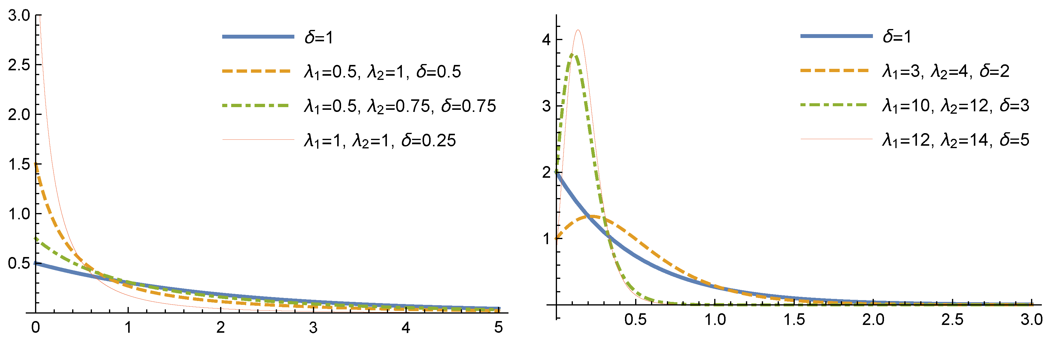
Remark 2.

If ${\lambda }_1={\lambda }_2,$ then (8) reduces to the Marsall–Olkin exponential distribution with parameters ${\lambda }_1$ and δ.

For several values of the parameters ${\lambda }_1,{\lambda }_2$ and $\delta ,$ the plots of the density function of GMOE distributions are shown in Figure 1.

Figure 1. Some probability density function (pdf) plots of generalised Marshall–Olkin exponential (GMOE) distributions for several values of $\delta$ parameter, $0<\delta \le 1$ (left panel) and $\delta \ge 1$ (right panel).

3. Some Properties of the GMO–Exponential Distribution

Some important properties of the $\mathrm{GMOE}\left({\lambda }_1,{\lambda }_2,\delta \right)$ distributions are shown in this section. From expression (3) and given $q\in (0,1)$ we can obtain the qth quantile $x_q$ of the GMOE distribution as follows. Let $q=G\left(x_q|{\lambda }_1,{\lambda }_2,\delta \right),$ that is,

$${\displaystyle q=1-\frac{\delta e^{-{\lambda }_1{x}_q}}{1-\left(1-\delta \right)e^{-{\lambda }_2{x}_q}}.}$$

Then, we rewrite this expression as

$${\displaystyle \left(1-\delta \right)\left(1-q\right)e^{-{\lambda }_2{x}_q}+\delta e^{-{\lambda }_1{x}_q}=\left(1-q\right),}$$

or equivalently

$$\left(1-\delta \right)\left(1-q\right)t_q^{{\lambda }_2}+\delta t_q^{{\lambda }_1}=\left(1-q\right),$$

(9)

where $t_q=e^{-x_q}$. Given the real solution of this equation, $t_q^{🟉}$, $x_q=-log\left(t_q^{🟉}\right)$ is the qth quantile of a $\mathrm{GMOE}\left({\lambda }_1,{\lambda }_2,\delta \right)$ distributed variable. Notice that Equation (9) has only one positive solution. Additionally, observe that this procedure is useful to obtain the quantile function of the GMOE distribution which is given by $Q\left(u\right)=-log\left(t\right(u\left)\right),$ where, when replacing q by u, $t\left(u\right)$ is the unique solution to (9). Therefore, if U is a uniform variate on the interval $(0,1)$, then the random variable $X=Q\left(U\right)$ has pdf (8).

3.1. Moments

The moments of a $\mathrm{GMO}$–exponential distribution can be written in a closed form with the help of the well-known Hurwitz–Lerch transcendent function, $\mathsf{\Phi }\left(z,s,a\right)$, which is defined by the expression

$${\displaystyle \mathsf{\Phi }\left(z,n,a\right)=\sum _{k=0}^{\infty }\frac{z^k}{{\left(k+a\right)}^n},}$$

and which can also be expressed in an integral form as follows:

$$\mathsf{\Phi }\left(z,n,a\right)=\frac{1}{\Gamma \left(n\right)}{\int }_0^{\infty }\frac{t^{n-1}{e}^{-at}}{1-z{e}^{-t}}dt.$$

(10)

Symbolic and numerical evaluations of this function are easily obtained with Mathematica${}^{\copyright }$ software using the command HurwitzLerchPhi.

Proposition 1.

The nth moment of the GMOE distribution is given by

$${\mu }_n=E\left(X^n\right)=\frac{\delta n!}{{\lambda }_2^n}\mathsf{\Phi }\left(1-\delta ,n,\frac{{\lambda }_1}{{\lambda }_2}\right).$$

(11)

Proof. 

Using expressions (8) and (10) and letting $t={\lambda }_{2}x$,

$$\begin{array}{lll}\hfill {\mu }_n& =& \delta {\int }_0^{\infty }\frac{t^n}{{\lambda }_2^n}\frac{\left(1-\delta \right)e^{-t}{e}^{-\frac{{\lambda }_1}{{\lambda }_2}t}}{{\left[1-\left(1-\delta \right)e^{-t}\right]}^2}dt+\delta {\int }_0^{\infty }\frac{{\lambda }_1{t}^n}{{\lambda }_2^{n+1}}\frac{e^{-\frac{{\lambda }_1}{{\lambda }_2}t}}{1-\left(1-\delta \right)e^{-t}}dt,\hfill \\ & =& \frac{\delta }{{\lambda }_2^n}{\int }_0^{\infty }{t}^n\frac{\left(1-\delta \right)e^{-t}{e}^{-\frac{{\lambda }_1}{{\lambda }_2}t}}{{\left[1-\left(1-\delta \right)e^{-t}\right]}^2}dt+\frac{{\lambda }_1\delta \Gamma \left(n+1\right)}{{\lambda }_2^{n+1}}\mathsf{\Phi }\left(1-\delta ,n+1,\frac{{\lambda }_1}{{\lambda }_2}\right).\hfill \end{array}$$

(12)

Now observe that ${\displaystyle {\int }_0^{\infty }\frac{t^n}{{\lambda }_2^n}\frac{\left(1-\delta \right)e^{-t}{e}^{-\frac{{\lambda }_1}{{\lambda }_2}t}}{{\left[1-\left(1-\delta \right)e^{-t}\right]}^2}dt}$ can be obtained by parts with

$${\displaystyle u=t^n{e}^{-\frac{{\lambda }_1}{{\lambda }_2}t}\mathrm{and}dv=\frac{\left(1-\delta \right)e^{-t}}{{\left[1-\left(1-\delta \right)e^{-t}\right]}^2}dt,}$$

and then

$$\begin{array}{ccc}\hfill \frac{\delta }{{\lambda }_2^n}{\int }_0^{\infty }{t}^n\frac{\left(1-\delta \right)e^{-t}{e}^{-\frac{{\lambda }_1}{{\lambda }_2}t}}{{\left[1-\left(1-\delta \right)e^{-t}\right]}^2}dt& =& \frac{\Gamma \left(n+1\right)\delta }{{\lambda }_2^n}\mathsf{\Phi }\left(1-\delta ,n,\frac{{\lambda }_1}{{\lambda }_2}\right)-\frac{\delta {\lambda }_1\Gamma \left(n+1\right)}{{\lambda }_2^{n+1}}\mathsf{\Phi }\left(1-\delta ,n+1,\frac{{\lambda }_1}{{\lambda }_2}\right).\hfill \end{array}$$

Substituting in (12) then gives

$${\displaystyle {\mu }_n=\frac{\Gamma \left(n+1\right)\delta }{{\lambda }_2^n}\mathsf{\Phi }\left(1-\delta ,n,\frac{{\lambda }_1}{{\lambda }_2}\right),}$$

and the proof is completed. □

Corollary 1.

Let X be a GMOE distribution with parameters ${\lambda }_1,{\lambda }_2$ and δ. Then,

(i) 

${\displaystyle {\mu }_n=n!\delta \sum _{k=0}^{\infty }\frac{{\left(1-\delta \right)}^k}{{\left({\lambda }_1+k{\lambda }_2\right)}^n}.}$

(ii) 

In particular,

$${\displaystyle E\left(X\right|{\lambda }_1,{\lambda }_2,\delta )=\frac{\delta }{{\lambda }_2}\mathsf{\Phi }(1-\delta ,1,\frac{{\lambda }_1}{{\lambda }_2}),}$$

(13)

$${\displaystyle Var\left(X\right|{\lambda }_1,{\lambda }_2,\delta )=\frac{{\delta }^2\mathsf{\Phi }{(1-\delta ,1,\frac{{\lambda }_1}{{\lambda }_2})}^2+2\delta \mathsf{\Phi }(1-\delta ,2,\frac{{\lambda }_1}{{\lambda }_2})}{{\lambda }_2^2}}$$

(14)

$${\kappa }_3=\frac{2{\delta }^3\mathsf{\Phi }{(1-\delta ,1,\frac{{\lambda }_1}{{\lambda }_2})}^3-6{\delta }^2\mathsf{\Phi }(1-\delta ,1,\frac{{\lambda }_1}{{\lambda }_2})\mathsf{\Phi }(1-\delta ,2,\frac{{\lambda }_1}{{\lambda }_2})+6\delta \mathsf{\Phi }(1-\delta ,3,\frac{{\lambda }_1}{{\lambda }_2})}{{\lambda }_2^3},$$

(15)

where ${\displaystyle {\kappa }_3=E\left({(X-\mu )}^3|{\lambda }_1,{\lambda }_2,\delta \right).}$

(iii) 

For a fixed value of $\delta >0,$ the value of its kth moment decreases with ${\lambda }_1$ and with ${\lambda }_2$.

Proof. 

The proof is immediate and (ii) follows from the identity $E\left({(X-\mu )}^k\right)={\sum }_{r=0}^k\left(\genfrac{}{}{0pt}{}{k}{r}\right)E\left(X^r\right){(-\mu )}^{k-r}.$ □

Using (13)–(15), the coefficient of variation (CV) and the skewness (${\gamma }_1$) of X are given by

$$CV=\sqrt{1+\frac{2}{\delta }\frac{\mathsf{\Phi }(1-\delta ,2,\frac{{\lambda }_1}{{\lambda }_2})}{\mathsf{\Phi }{(1-\delta ,1,\frac{{\lambda }_1}{{\lambda }_2})}^2}},$$

(16)

$${\gamma }_1=\frac{2{\delta }^3\mathsf{\Phi }{(1-\delta ,1,\frac{{\lambda }_1}{{\lambda }_2})}^3-6{\delta }^2\mathsf{\Phi }(1-\delta ,1,\frac{{\lambda }_1}{{\lambda }_2})\mathsf{\Phi }(1-\delta ,2,\frac{{\lambda }_1}{{\lambda }_2})+6\delta \mathsf{\Phi }(1-\delta ,3,\frac{{\lambda }_1}{{\lambda }_2})}{{\left({\delta }^2\mathsf{\Phi }{(1-\delta ,1,\frac{{\lambda }_1}{{\lambda }_2})}^2+2\delta \mathsf{\Phi }(1-\delta ,2,\frac{{\lambda }_1}{{\lambda }_2})\right)}^{3/2}}.$$

(17)

Observe that in GMOE distributions with a constant ${\lambda }_1/{\lambda }_2$ ratio, the $CV$ and ${\gamma }_1$ only depend on $\delta$.

3.2. The Hazard Rate: Reliability Properties

The hazard rate of a $\mathrm{GMOExp}\left({\lambda }_1,{\lambda }_2,\delta \right)$ distribution, $r\left(x|{\lambda }_1,{\lambda }_2,\delta \right)$, is given by

$$r\left(x|{\lambda }_1,{\lambda }_2,\delta \right)=\frac{\left(1-\delta \right)\left({\lambda }_2-{\lambda }_1\right)e^{-{\lambda }_{2}x}+{\lambda }_1}{1-\left(1-\delta \right)e^{-{\lambda }_{2}x}}.$$

(18)

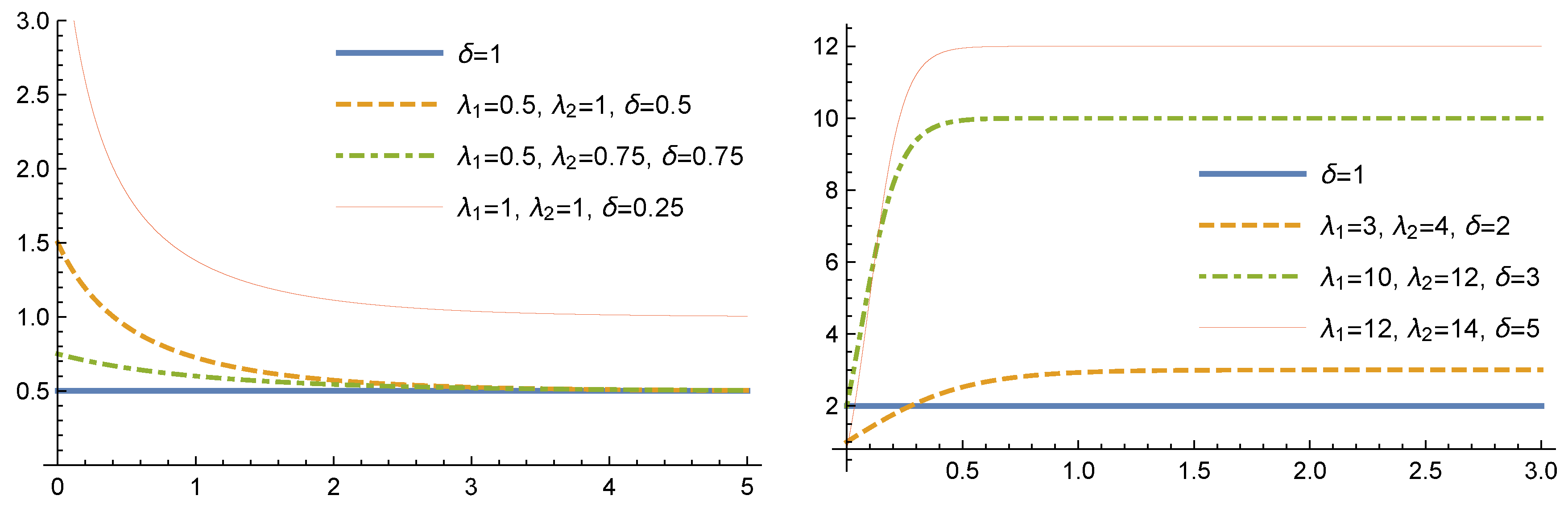
As Figure 2 shows, the hazard rate function of the GMOE distribution can take monotonic and quasi-bathtub shapes for different values of the parameters ${\lambda }_1,{\lambda }_2$ and $\delta .$

Figure 2. Some hazard rate plots of GMOE distributions for several values of $\delta$ parameter, $0<\delta \le 1$ (left panel) and $\delta \ge 1$ (right panel).

If we denote by $r_E\left(x|\lambda \right)$ the hazard rate of an $Exp\left(\lambda \right)$ distribution, the following results can be obtained immediately:

Proposition 2. 

(i) 

For all ${\lambda }_2>0,$

$$r\left(x|{\lambda }_1,{\lambda }_2,\delta \right)>r_E\left(x|{\lambda }_1\right)iff0<\delta <1.$$

(ii) 

For $x>0,$

$$r\left(x|{\lambda }_1,{\lambda }_2,\delta \right)>r_E\left(x|{\lambda }_2\right)iff{\lambda }_1\left[1-\left(1-\delta \right)e^{-{\lambda }_{1}x}\right]>{\lambda }_2\left[1-2\left(1-\delta \right)e^{-{\lambda }_{2}x}\right],$$

(iii) 

$r\left(x|{\lambda }_1,{\lambda }_2,\delta \right)$ is a strictly decreasing function for $0<\delta <1,$ constant for $\delta =1$ and strictly increasing for $\delta >1.$

Proof. 

(i) and (ii) are immediate. For (iii), the result follows by observing that the sign of the first derivative of the hazard rate function in (9) with respect to x is the opposite to the sign of $1-\delta$. □

Furthermore, $r(·|{\lambda }_1,{\lambda }_2,\delta )$ is increasing in ${\lambda }_1$ and in $\delta .$ Thus, the GMOE distribution is positively ordered with respect to ${\lambda }_1$ according to the hazard rate ordering, and analogously, with respect to $\delta .$

In contrast with the ordinary families of gamma and Weibull distributions, observe that ${\displaystyle \underset{x\to 0}{lim}r\left(x\right|{\lambda }_1,{\lambda }_2,\delta )=\frac{(1-\delta )({\lambda }_2-{\lambda }_1)+{\lambda }_1}{\delta },}$ and that at the origin the hazard rate varies continuously with the parameters. Moreover, for the GMOE distribution, ${\displaystyle \underset{x\to \infty }{lim}r\left(x\right|{\lambda }_1,{\lambda }_2,\delta )={\lambda }_1}$, is bounded and continuous in the parameters.

Finally, the residual life distribution of the random variable X—distributed as a GMOE distribution with the parameters ${\lambda }_1,{\lambda }_2$ and $\delta$—provided there is no failure prior to time $t>0,$ has the survival function

$$\begin{array}{lll}{S}_t\left(x\right|{\lambda }_1,{\lambda }_2,\delta )\hfill & =& Pr\left(X>x+t|X>t\right)=e^{-{\lambda }_{1}x}\frac{1-(1-\delta )e^{-{\lambda }_{2}t}}{1-(1-\delta )e^{-{\lambda }_2(x+t)}}\hfill \\ & =& \frac{\beta \left(t\right)e^{-{\lambda }_{1}x}}{1-(1-\beta \left(t\right))e^{-{\lambda }_{2}x}}=S\left(x\right|{\lambda }_1,{\lambda }_2,\beta \left(t\right)),\hfill \end{array}$$

where $\beta \left(t\right)=1-(1-\delta )e^{-{\lambda }_{2}t}.$ Thus, the residual life distribution of a random variable X distributed as $\mathrm{GMOE}({\lambda }_1,{\lambda }_2,\delta )$ at time t is another GMOE distribution with the third parameter depending upon time $t.$

Henceforth, from (12) the mean residual life function, i.e., the mean of the residual life distribution, is given by

$$m\left(t\right|{\lambda }_1,{\lambda }_2,\delta )=\frac{\beta \left(t\right)}{{\lambda }_2}\mathsf{\Phi }(1-\beta \left(t\right),1,\frac{{\lambda }_1}{{\lambda }_2}).$$

(19)

It is then easy to see that

$$\underset{t\to \infty }{lim}m\left(t\right|{\lambda }_1,{\lambda }_2,\delta )=\frac{1}{{\lambda }_1}=E\left(X\right|{\lambda }_1,{\lambda }_2,1)if\delta <1,$$

and

$$\underset{t\to 0}{lim}m\left(t\right|{\lambda }_1,{\lambda }_2,\delta )=\frac{\delta }{{\lambda }_2}\mathsf{\Phi }(1-\delta ,1,\frac{{\lambda }_1}{{\lambda }_2})=E\left(X\right|{\lambda }_1,{\lambda }_2,\delta ).$$

3.3. The Mode

From Remarks 1 and 2 in Section 2, we now focus on the values of $\delta >0$ and $\delta \ne 1.$ The GMOE distribution can present its unique mode either at $M=0$ or at $M>0.$

Let us define the function

$$h\left(x\right)=\frac{1}{\delta }g\left(x|{\lambda }_1,{\lambda }_2,\delta \right),$$

(20)

such that

$${\displaystyle h^{\prime }\left(x\right)=\frac{dh\left(x\right)}{dx}=\frac{h_1\left(x\right)+h_2\left(x\right)}{{\left(1-\left(1-\delta \right)e^{-{\lambda }_{2}x}\right)}^3},}$$

where

$$h_1\left(x\right)=\left(-\left(1-\delta \right)\left({\lambda }_2^2-{\lambda }_1^2\right)e^{-{\lambda }_{2}x-{\lambda }_{1}x}-{\lambda }_1^2{e}^{-{\lambda }_{1}x}\right)\left(1-\left(1-\delta \right)e^{-{\lambda }_{2}x}\right)$$

and

$$h_2\left(x\right)=-2\left(\left(1-\delta \right)\left({\lambda }_2-{\lambda }_1\right)e^{-{\lambda }_{2}x-{\lambda }_{1}x}+{\lambda }_1{e}^{-{\lambda }_{1}x}\right)\left(1-\delta \right){\lambda }_2{e}^{-{\lambda }_{2}x}.$$

Now, to determine whether there exists a positive mode we need merely decide whether $h^{\prime }\left(0\right)>0$:

$${\displaystyle h^{\prime }\left(0\right)=\frac{-{\delta }^2{\lambda }_1^2-\left(\delta -1\right)\left(\delta -2\right){\lambda }_2^2+2\delta \left(\delta -1\right){\lambda }_2{\lambda }_1}{{\delta }^3}>0,}$$

or equivalently,

$$-{\delta }^2{\lambda }_1^2-\left(\delta -1\right)\left(\delta -2\right){\lambda }_2^2+2\delta \left(\delta -1\right){\lambda }_2{\lambda }_1>0.$$

Assuming $t={\lambda }_2/{\lambda }_1$, we define the auxiliary function as

$$N\left(t,\delta \right)=-\left(\delta -1\right)\left(\delta -2\right)t^2-2\delta \left(1-\delta \right)t-{\delta }^2,$$

(21)

Hence, in order to find the mode of GMOE distribution we need only decide whether $N(t,\delta )>0.$ The solution to this question depends on the range of values for $\delta$.

(Case a)

If $0<\delta <1$, $N\left(t,\delta \right)<0$ for any $t\ge 0$, and therefore the mode of distribution $\mathrm{GMOE}\left({\lambda }_1,{\lambda }_2,\delta \right)$ is reached at $M=0$

(Case b)

If $1<\delta <2,$

$$N\left(t,\delta \right)=\left(\delta -1\right)\left(2-\delta \right)t^2+2\delta \left(\delta -1\right)t-{\delta }^2>0,$$

implies one of the following two cases. On the one hand,

$${\displaystyle t<s_1=\frac{-\delta \left(\delta -1\right)-\delta \sqrt{\delta -1}}{\left(\delta -1\right)\left(2-\delta \right)}<0,}$$

which is contradictory, and on the other hand,

$${\displaystyle t>s_2=\frac{-\delta \left(\delta -1\right)+\delta \sqrt{\delta -1}}{\left(\delta -1\right)\left(2-\delta \right)}>0;}$$

that is,

$${\displaystyle \frac{\delta \sqrt{\delta -1}-\delta \left(\delta -1\right)}{\left(\delta -1\right)\left(2-\delta \right)}{\lambda }_1<{\lambda }_2.}$$

However, for $1<\delta <2$, the inequality

$${\displaystyle \frac{\delta \sqrt{\delta -1}-\delta \left(\delta -1\right)}{\left(\delta -1\right)\left(2-\delta \right)}>\frac{\delta }{\delta -1}}$$

never holds. In summary, we conclude that the mode is reached at $M=0$ in this case.

(Case c)

If $\delta =2$, the condition reduces to $t>1$, or equivalently ${\lambda }_1<{\lambda }_2\le 2{\lambda }_1$.

(Case d)

Finally, if $\delta >2$, $N\left(t,\delta \right)=-\left(\delta -1\right)\left(\delta -2\right)t^2+2\delta \left(\delta -1\right)t-{\delta }^2>0$ implies

$${\displaystyle 0<s_1=\frac{\delta \left(\delta -1\right)-\delta \sqrt{\left(\delta -1\right)}}{\left(\delta -1\right)\left(\delta -2\right)}<t<s_2=\frac{\delta \left(\delta -1\right)+\delta \sqrt{\left(\delta -1\right)}}{\left(\delta -1\right)\left(\delta -2\right)}.}$$

Notice that, for any $\delta >2$,

$${\displaystyle s_1<\frac{\delta }{\delta -1}<s_2,}$$

so we conclude that, in this case, $M>0$ if and only if

$${\displaystyle \frac{\delta \left(\delta -1\right)-\delta \sqrt{\left(\delta -1\right)}}{\left(\delta -1\right)\left(\delta -2\right)}{\lambda }_1<{\lambda }_2\le \frac{\delta }{\delta -1}{\lambda }_1.}$$

3.4. Order Statistics

Let $X_1,\dots ,X_n$ be a random sample of size n from the GMOE distribution in (8). Then, the density of the jth order statistics $X_{j:n},$ for $j=1,\dots ,n,$ is given by

$$g_{j:n}\left(x\right|{\lambda }_1,{\lambda }_2,\delta )=\frac{n!}{(j-1)!(n-j)!}\frac{k_{j:n}\left(x\right|{\lambda }_1,{\lambda }_2,\delta )}{{\left(1-(1-\delta )e^{-{\lambda }_{2}x}\right)}^{n+1}},$$

(22)

where

$$\begin{array}{ccc}{k}_{j:n}\left(x\right|{\lambda }_1,{\lambda }_2,\delta )\hfill & =& {\left(1-(1-\delta )e^{-{\lambda }_{2}x}-\delta e^{-{\lambda }_{1}x}\right)}^{j-1}{\left(\delta e^{-{\lambda }_{1}x}\right)}^{n-j}\hfill \\ & & \times \left(\delta (1-\delta )({\lambda }_2-{\lambda }_1)e^{-({\lambda }_2+{\lambda }_1)x}+\delta {\lambda }_1{e}^{-{\lambda }_{1}x}\right)\hfill \end{array}$$

In particular, the sample distributions of the minimum $X_{1:n}$ and maximum $X_{n:n}$ are easily obtained by (22) replacing j by 1 and $n,$ respectively.

4. Estimation

In this section, we estimate the unknown parameters of the GMOE distribution. Let $\underline{\mathbf{x}}=(x_1,\dots ,x_n)$ be a sample of size n from the GMOE distribution in (8). The log-likelihood function for the parameters $({\lambda }_1,{\lambda }_2,\delta )$ is expressed as

$$\begin{array}{ccc}\hfill l\left(\underline{\mathbf{x}}|\mathit{\alpha }\right)& =& nlog\delta +\sum _{i=1}^{n}log\left(\left(1-\delta \right)\left({\lambda }_2-{\lambda }_1\right)e^{-\left({\lambda }_2+{\lambda }_1\right)x_i}+{\lambda }_1{e}^{-{\lambda }_1{x}_i}\right)\hfill \\ & & -2\sum _{i=1}^{n}log\left(1-\left(1-\delta \right)e^{-{\lambda }_2{x}_i}\right),\hfill \end{array}$$

where $\mathit{\alpha }=({\lambda }_1,{\lambda }_2,\delta ).$ By differentiating with respect to ${\lambda }_1,{\lambda }_2$ and $\delta$ and then equating to zero, we obtain the normal equations needed to estiate the maximum likelihood.

$$\begin{array}{ccc}\hfill \frac{\partial l\left(\underline{\mathbf{x}}|\mathit{\alpha }\right)}{\partial \delta }& =& \frac{n}{\delta }+\sum _{i=1}^n\frac{{\lambda }_1-{\lambda }_2}{\left(1-\delta \right){\lambda }_2-\left(1-\delta -e^{{\lambda }_2{x}_i}\right){\lambda }_1}+\sum _{i=1}^n\frac{2}{1-\delta -e^{{\lambda }_2{x}_i}},\hfill \end{array}$$

(23)

$$\begin{array}{ccc}\hfill \frac{\partial l\left(\underline{\mathbf{x}}|\mathit{\alpha }\right)}{\partial {\lambda }_1}& =& -\sum _{i=1}^n\frac{\left(1-\delta \right)\left[1-\left({\lambda }_1-{\lambda }_2\right)x_i\right]-\left(1-{\lambda }_1{x}_i\right)e^{{\lambda }_2{x}_i}}{\left(1-\delta \right){\lambda }_2-\left(1-\delta -e^{{\lambda }_2{x}_i}\right){\lambda }_1},\hfill \end{array}$$

(24)

$$\begin{array}{ccc}\hfill \frac{\partial l\left(\underline{\mathbf{x}}|\mathit{\alpha }\right)}{\partial {\lambda }_2}& =& \sum _{i=1}^n\frac{\left(1-\delta \right)\left[1+\left({\lambda }_1-{\lambda }_2\right)x_i\right]}{\left(1-\delta \right){\lambda }_2-\left(1-\delta -e^{{\lambda }_2{x}_i}\right){\lambda }_1}+\sum _{i=1}^n\frac{2\left(1-\delta \right)x_i}{1-\delta -e^{{\lambda }_2{x}_i}}.\hfill \end{array}$$

(25)

These non–linear equations do not have a closed expression, but require numerical methods, available in standard software such as Mathematica.

The pdf of the GMOE distribution in (8) satisfies all the regularity conditions, and thus from the usual, large sample approximation, the MLE $({\widehat{\lambda }}_1,{\widehat{\lambda }}_2,\widehat{\delta })$ treated as being approximately multivariate normal with a mean vector $({\lambda }_1,{\lambda }_2,\delta )$ and variance–covariance matrix $I^{-1},$ and where the elements are provided by the inverse Fisher information matrix, the expected values of the second order derivatives are as shown in Appendix A.

4.1. Simulation Study

In this section, we evaluate the performance of the MLEs and Bayesian estimators using Monte Carlo simulation, for certain sample sizes and parameter values. The simulation study is repeated $N=1000$ times with sample sizes $n=25,50,100.$ Table 1 shows the results obtained for different parameter combinations, together with the estimated bias and root mean squared error (RMSE) for each estimated parameter given a simulated sample of size n, using the common expressions

$${\displaystyle \mathrm{Bias}=\frac{1}{N}\sum _{i=1}^N({\widehat{\alpha }}_i-\alpha )\mathrm{and}\mathrm{RMSE}=\sqrt{\frac{1}{N}{\sum }_{i=1}^N{({\widehat{\alpha }}_i-\alpha )}^2}.}$$

Table 1. MLEs and MCMC results. Scenario I: ${\lambda }_1=0.5,{\lambda }_2=1,\delta =0.5$.

n	Parameter	Mean	Bias	RMSE
25	${\lambda }_1$	0.56	0.19	0.63
	${\lambda }_2$	0.98	6.76	61.96
	$\delta$	0.58	6908.21	>10${}^5$
50	${\lambda }_1$	0.54	0.07	0.37
	${\lambda }_2$	1.01	2.18	9.74
	$\delta$	0.55	3814.02	>10${}^5$
100	${\lambda }_1$	0.51	0.016	0.19
	${\lambda }_2$	1.003	1.11	5.25
	$\delta$	0.52	221.236	>10${}^3$

Table 1 shows that the parameter estimators perform very badly, mainly due to the nonlinearity and instability of the solutions to Equations (23)–(25), even for large values of n. The above three likelihood equations are very complicated, and the Newton–Raphson method is a gradient procedure whose stability depends on the selection of the initial solutions. It is not easy to set up good initial solutions to these three equations. An alternative procedure to obtain stable MLE consists of developing a non-informative Bayesian estimation approach. Doing so, we employ the MCMC method to generate samples from the posterior distributions of the parameters ${\lambda }_1,{\lambda }_2$ and $\delta$ from independent, uniform vague priors and then compute the corresponding Bayes estimators using the common squared errors loss function. From Table 2 it is clear that MCMC samples can be used to estimate the parameters in GMOE distributions and that this method obtains better results than solving the normal equations directly by maximum likelihood. A simple code implemented using OpenBUGS is given in Appendix B. The summary statistics shown in Table 2 are based on $N=1000$ simulations with 50,000 iterations following a burn-in stage of 5000 iterations.

Table 2. MCMC Bayesian estimation.

n	Parameter	Mean	Bias	RMSE	StD
Scenario I : ${\lambda }_1=0.5,{\lambda }_2=1,\delta =0.5$
25	${\lambda }_1$	0.60	0.10	0.62	0.13
	${\lambda }_2$	0.99	−0.01	0.99	0.15
	$\delta$	0.57	0.06	0.57	0.10
50	${\lambda }_1$	0.58	0.08	0.59	0.13
	${\lambda }_2$	1.02	−0.01	1.03	0.17
	$\delta$	0.55	0.05	0.56	0.10
100	${\lambda }_1$	0.54	0.07	0.55	0.10
	${\lambda }_2$	1.007	−0.01	1.08	0.18
	$\delta$	0.53	0.05	0.53	0.08
Scenario II : ${\lambda }_1=1.5,{\lambda }_2=2.0,\delta =0.5$
25	${\lambda }_1$	1.79	9.29	1.83	0.39
	${\lambda }_2$	1.92	−0.08	1.93	0.26
	$\delta$	0.58	0.07	0.58	0.10
50	${\lambda }_1$	1.74	0.24	1.78	0.37
	${\lambda }_2$	1.96	−0.03	1.98	0.28
	$\delta$	0.57	0.07	0.58	0.10
100	${\lambda }_1$	1.65	0.16	1.68	0.31
	${\lambda }_2$	2.07	0.07	2.09	0.27
	$\delta$	0.55	0.05	0.56	0.09

5. Numerical Illustrations

5.1. Example 1

Here, we revisit the real dataset from [4] representing the number of revolutions before failure for each of the 23 bearings in the life test described in Table 3.

Table 3. Dataset in Gupta and Kundu [4].

17.88	45.60	55.56	84.12	127.92
28.92	48.40	67.80	93.12	128.04
33.00	51.84	68.64	98.64	173.40
41.52	51.96	68.64	105.12
42.12	54.12	68.88	105.84

Table 4 shows the fits to the dataset obtained from the three-parameter gamma, Weibull and GMOE models, whose probability density functions are given as follows.

Table 4. Estimated parameters, log-likelihood, K-S statistics, p-values, AIC and BIC for Example 1.

	Models
	Gamma	Weibull	4–Parameters Gamma	GMOE
	$(\widehat{\alpha },\widehat{\beta },\widehat{\gamma })$	$(\widehat{\alpha },\widehat{\beta },\widehat{\mu })$	$(\widehat{\alpha },\widehat{\beta },\widehat{\gamma },\widehat{\mu })$	$({\widehat{\lambda }}_1,{\widehat{\lambda }}_2,\widehat{\delta })$
Estimation	$(10.5669,1.3796,0.6032)$	$(1.59,63.8723,14.8783)$	$(0.7038,79.1267,1.8884,16.3264)$	$(0.0359,0.0412,7.8156)$
Loglikelihood	$-112.97$	$-112.85$	$-112.847$	$-113.42$
${\chi }^2$(d.f.)	5.1739 (2)	3.7826 (2)	3.782 (3)	3.00 (2)
p-value	0.6387	0.8044	0.804	0.223
BIC	235.345	235.107	238.224	236.26
AIC	231.938	231.70	283.682	232.85

5.1.1. Four (Three)-Parameter Gamma Distribution

$${\displaystyle g\left(x\right|\alpha ,\beta ,\gamma ,\mu )=\frac{1}{\beta \Gamma \left(\alpha \right)}·\gamma ·{\left(\frac{x-\mu }{\beta }\right)}^{\alpha ·\gamma -1}exp\left\{-{\left(\frac{x-\mu }{\beta }\right)}^{\gamma }\right\},x>\mu ,}$$

with shape parameters $\alpha$ and $\gamma$, scale parameter $\beta ,$ and location parameter $\mu .$ This gamma distribution allows $\alpha$, $\beta$ and $\gamma$ to be any positive real numbers, and $\mu$ to be any real number. The three-parameter gamma distribution $g\left(x\right|\alpha ,\beta ,\gamma )$ is equivalent to $g\left(x\right|\alpha ,\beta ,\gamma ,0).$

5.1.2. Three-Parameter Weibull Distribution

$${\displaystyle g\left(x\right|\alpha ,\beta ,\mu )=\frac{1}{\beta }·\alpha ·{\left(\frac{x-\mu }{\beta }\right)}^{\alpha -1}exp\left\{-{\left(\frac{x-\mu }{\beta }\right)}^{\alpha }\right\},x>\mu .}$$

This pdf represents a three-parameter Weibull distribution with shape parameter $\alpha$, scale parameter $\beta ,$ and location parameter $\mu ,$ where $\alpha$ and $\beta$ are positive real numbers and $\mu$ is any real number.

For comparative and illustrative purposes, all the usual measures, such as p-value, log-likelihood, AIC and BIC, are used to compare the estimated models. As is well known, a model with a minimum BIC value is to be preferred. From Table 4, the log-likelihood and BIC quantities show that, excluding the four-parameter gamma distribution, the remaining three models are almost identical. Table 4 shows that the GMOE distribution performs well in fitting the data distribution when there is a decreasing hazard rate function, and provides a fit as good as that of the three-parameter common distribution. Thus, GMOE distributions could be included in the catalogue of sampling distributions for this kind of dataset.

5.2. Example 2

The data for this example were compiled by the Swedish Committee on the Analysis of Risk Premium in Motor Insurance, summarised in Hallin and Ingenbleek [19] and Andrews and Herzberg [20]. The data correspond to third party automobile insurance claims for the year 1977, and are available at the url [21]. We consider the sums of payments (the severity), in Swedish krona.

The histogram and the empirical hazard function for the data are shown in Figure 3. Observe that the monotonic decreasing of the hazard function suggests that a generalised exponential distribution fits the data well.

Figure 3. Ordinary histogram (left panel) and empirical hazard function (right panel) of data in Example 2.

We fitted three models to these data: exponential (E), Marshall and Olkin exponential (MOE) and GMOE. Table 5 shows the fit of each of these models to the data set. For comparison, log-likelihood, BIC and AIC values are also presented, together with the estimation of the parameters by the maximum likelihood method. In the GMOE model, the stability of the MLE was confirmed by the non-informative Bayesian procedure described in Section 4.1 using uniform vague priors centred at the MLE obtained and solving (23)–(25). For the data set considered, all of the BIC and AIC values indicate that the GMOE model is better.

Table 5. Estimated parameters, Loglikelihood, AIC and BIC for Example 2.

	Models
	>Exponential	MOE	GMOE
	$\widehat{\alpha }$	$(\widehat{\lambda },\widehat{\delta })$	$({\widehat{\lambda }}_1,{\widehat{\lambda }}_2,\widehat{\delta })$
Estimation	$3.80153\times {10}^{-6}$	$(1.96183\times {10}^{-7},0.003135)$	$(3.12557\times {10}^{-6},4286.3,0.783562)$
Loglikelihood	$-29,022.7$	$-\mathrm{26,638.8}$	$-\mathrm{21,927.9}$
BIC	58,053.1	53,292.9	43,878.8
AIC	58,047.4	53,281.6	43,861.8

6. Extensions of the GMO Scheme

In this Section, we show some general properties of the $\mathrm{GMO}$ scheme applied to any absolutely continuous distribution. Consider a pair of absolutely continuous distributions, denoted by $F_i\left(x\right),$$S_i\left(x\right)$ and $f_i\left(x\right)$, for $i=1,2$, their respective cdfs, survival and pdfs’ functions. We assume that each $F_i\left(x\right)$ depends on its parameter ${\theta }_i,i=1,2$. We then define the survival function of the $\mathrm{GMO}$ with respect to $\left(F_1,F_2\right)$ as the function

$${\displaystyle S\left(x|{\theta }_1,{\theta }_2,\delta \right)=\frac{\delta S_1\left(x\right)}{1-\left(1-\delta \right)S_2\left(x\right)},}$$

The corresponding cdf is then given by

$$\begin{array}{ccc}\hfill G\left(x|{\theta }_1,{\theta }_2,\delta \right)& =& 1-\frac{\delta S_1\left(x\right)}{1-\left(1-\delta \right)S_2\left(x\right)}=\frac{\delta F_1\left(x\right)+\left(1-\delta \right)F_2\left(x\right)}{\delta +\left(1-\delta \right)F_2\left(x\right)}.\hfill \end{array}$$

and the corresponding pdf, by

$${\displaystyle g\left(x|{\theta }_1,{\theta }_2,\delta \right)=\frac{\delta \left(1-\delta \right)f_2\left(x\right)S_1\left(x\right)+{\delta }^2{f}_1\left(x\right)+\delta \left(1-\delta \right)F_2\left(x\right)f_1\left(x\right)}{{\left[\delta +\left(1-\delta \right)F_2\left(x\right)\right]}^2},}$$

We require that $g\left(x|{\theta }_1,{\theta }_2,\delta \right)\ge 0$ for all x. Clearly, in the case $0<\delta \le 1$, this condition is always met. On the other hand, when $\delta >1$, the required condition reduces to

$${\displaystyle f_1\left(x\right)\ge \left(\delta -1\right)\left(f_2\left(x\right)S_1\left(x\right)-S_2\left(x\right)f_1\left(x\right)\right).}$$

7. Conclusions

In this paper, we propose an extension of the Marshall–Olkin procedure to obtain a new three-parameter distribution with a monotone hazard rate function and describe some interesting properties that could be used in reliability scenarios. We show that the proposed distribution can be considered a valid alternative to well-known distributions, such as the Marsall–Olkin exponential and generalised gamma and Weibull distributions, among many others. The cumulative distribution function (cdf) and the hazard rate function present great flexibility. The nth moment is derived and particular values for the mean, variance and kurtosis are easily obtained. The non-linear equations for deriving the MLE and the elements of the observed information matrix are also presented. It can be seen that the maximum-likelihood method can be applied by running a MCMC procedure with non–informative uniform priors. This approach can also be applied to other distributions, although not to exponential ones. An application of the GMOE distribution to two real data sets is provided to demonstrate that this distribution provides a suitable alternative to the standard models.