A New Method for Dynamic Multi-Objective Optimization Based on Segment and Cloud Prediction

Abstract

In the real world, multi-objective optimization problems always change over time in most projects. Once the environment changes, the distribution of the optimal solutions would also be changed in decision space. Sometimes, such change may obey the law of symmetry, i.e., the minimum of the objective function in such environment is its maximum in another environment. In such cases, the optimal solutions keep unchanged or vibrate in a small range. However, in most cases, they do not obey the law of symmetry. In order to continue the search that maintains previous search advantages in the changed environment, some prediction strategy would be used to predict the operation position of the Pareto set. Because of this, the segment and multi-directional prediction is proposed in this paper, which consists of three mechanisms. First, by segmenting the optimal solutions set, the prediction about the changes in the distribution of the Pareto front can be ensured. Second, by introducing the cloud theory, the distance error of direction prediction can be offset effectively. Third, by using extra angle search, the angle error of prediction caused by the Pareto set nonlinear variation can also be offset effectively. Finally, eight benchmark problems were used to verify the performance of the proposed algorithm and compared algorithms. The results indicate that the algorithm proposed in this paper has good convergence and distribution, as well as a quick response ability to the changed environment.

1. Introduction

Dynamic multi-objective optimization problems (DMOOPs) belong to a kind of time-varying multi-objective optimization problems that is frequently encountered in the disciplines of science and engineering. These problems not only display the conflict in optimization targets and high dimension in solution space, but also have the time-varying characteristics in optimization objective, constraints, and decision space [1,2,3,4,5,6,7]. As a result, the high conditionality of traditional algorithms makes it difficult to meet requirements about large-scale, high timeliness and complex non-deterministic polynomial (NP) hard problems. Compared with traditional algorithms, evolution methods have low requirements in problem model, high efficiency, as well as embarrassingly parallel self-organizing and self-adaption, so they have been widely used in the modern industry and scientific research field [8,9,10].

The easiest way is to keep the diversity of the population in evolution methods used to solve DMOOPs. For example, DNSGA-II (dynamic multi-objective optimization and decision-making using the modified NSGA-II) proposed by Deb [11] uses partial random initialization or random variation in order to enhance the flexibility of the population in the changed environment. Moreover, three immigration schemes proposed by Azevedo are used to initialize the population in the changed environment [12], as well as the immune clonal algorithm proposed by Shang Rong-hua [13]. Because of the unknown variation trend for the dynamic environment, those methods can be formulated into an attempted exploration method, which could ensure the superiority individual could be reserved in the changed environment. The upside for these methods is that they can adapt to a variety of changing environments, while their downside is that advantages of search before environmental change would be difficult to keep after change. Thus, the characteristics of this kind of methods are their powerful environmental adaptability and poor prediction accuracy.

Compared with the early methods, by maintaining the diversity of the population, historical information from multiple environmental changes is used to predict the position of the population in the next environmental change. That is, it is a type of statistical method to study the non-dominate solution set. There are two solutions for this, namely the memory strategy and the prediction strategy.

The memory strategy predicts the position of the population in the next environmental change by rules, which stores a lot of information about non-dominate solution set. The memory strategy is suited to solve the dynamic problem of “short periodicity”. Here, “Periodicity” could be described by the historical information, and “short” indicates less storage [14,15,16].

However, this has several drawbacks, namely large memory consumption and incorrect predictions to solve time-varying nonlinear problems or more frequent environmental changes.

The prediction strategy uses historical information by statistical analysis and predicts the possible direction of population migration using prediction theory (for example, linear regression, autoregressive model, etc.), relative to the memory strategy. The FPS (feed-forward prediction strategy) proposed by Hatzakis [17] is used to predict the migration locations of the non-dominant solution set, which is based on an autoregressive model. Because of the incomplete statistical analysis about historical information, the FPS is weak and ineffective. The PPS (population prediction strategy) proposed by Zhou [18] uses an autoregressive model to predict the central migration locations of the population, and shape estimation to migrate the whole population. Compared with the FPS, the PPS has mainly two characteristics: (1) further treatment of historical information, which is used to predict the central locations of the population; and (2) shape estimation, which is better than estimation one by one. All of these methods based on autoregressive model have a fundamental disadvantage, namely, a large amount of statistical information is needed to construct the model. Moreover, if the prediction error is increasing repeatedly, the prediction error will be amplified. As a result, it is difficult to adjust when the change rule of the environment is changed.

In short, the autoregressive model is widely used to solve regular change problems, but has the problems of slow response speed and large amounts of statistical data. To compensate, the diversity-keeping strategy is widely used. The DSS (directed search strategy) proposed by Wu [19] is used to solve the dynamic problem, which uses both central population prediction and cross search. Moreover, the method of population center prediction is a linear prediction. Compared with MLR (multiple linear regression), it needs less historical information and has a better adaptive capacity to the environment. For DMOOPS, a method proposed by Rong [20] is used to predict the changes, which uses a linear model based on segmentation of the optimal front. Furthermore, the linear model used by Li [21] is based on the prediction of the autoregressive model. It predicts the key points of the optimal front, such as the boundary point, inflection point, etc. Also, the linear model is used by Ruan [22] to predict the position of the optimal front. In maintaining population diversity, the changes in population are predicted based on the extreme point of the previous generation [20]. However, it is worth noting that the prediction error should always exist in the linear model when solving dynamic problems (progressive increase, progressive decrease, or more complex changes). Therefore, all the literature above employs the diversity keeping scheme to redress prediction errors.

According to the problem of remedying the shortage of the linear model, the segmentation cloud predict strategy (SCPS) is proposed in this paper to improve the precision of prediction. First, the searched optimal front would be segmented to divide the population. Second, a new linear prediction analysis is applied to each part of the population, which would draw on the thoughts of the cloud model. According to the notion of uncertain time in the cloud model, entropy (or super entropy) would be used to redress the prediction errors. Moreover, for some abrupt nonlinear changes in dynamic problems, the extra angle search strategy is used to ensure the diversity of the population during the prediction process.

The rest of this paper is organized as follows. The problem of dynamic multi-objective is described in Section 2. The segmentation cloud prediction strategy is proposed in Section 3. Benchmark problems are applied in Section 4 to show the performance of the proposed method, together with related experimental analysis. Conclusions are provided in the last section.

2. Description of Dynamic Multi-Objective Problem

Considering the symmetry between minimum and maximum under symmetric environments, the optimization problem can be normalized to a unit form. Generally, the DMOP could be described as follows,

$$\{\begin{array}{l}minF(x,t)=\left(f_1\right(x,t),\dots ,f_m(x,t){)}^T\\ s.t.g(v,t)\le 0,h(v,t)=0\end{array}$$

(1)

where the decision variables are $x={(x_1,\dots ,x_n)}^T\in \mathsf{\Omega }$, $\mathsf{\Omega }$ is the n dimension decision space, and the time variable is t. $g(v,t)$ is the equality constraint, while $h(v,t)$ is the inequality constraint. The objective function vector is $y={(f_1,\dots ,f_m)}^T\in \mathsf{\Lambda }$, and $\mathsf{\Lambda }$ is the m dimension decision space. The evaluation function $F(x,t):\mathsf{\Omega }\times T\to \mathsf{\Lambda }$ would define the mapping from decision space to object space [23].

Definition 1.

(Pareto domination). For some time t, if individual p, it can as $p\prec q$. If and only if $\forall i=\{1,2,\dots ,m\}$: $f_i(p,t)\le f_i(q,t)$, $\exists \mathrm{j}=\{1,2,\dots ,m\}$:$f_j(p,t)<f_j(q,t)$.

Definition 2.

(Pareto optimal solution set, PS). Let $x\in \mathsf{\Omega }$, which is the decision variable. PS could be defined as follows,

$$\mathrm{PS}:=\{x\in \mathsf{\Omega }|\neg \exists y\in \mathsf{\Omega },y\prec x\}$$

(2)

Definition 3.

(Pareto optimal front, PF). Let $x\in \mathsf{\Omega }$, which is the decision variable. PF could be defined as follows,

$$\mathrm{PF}:=\{y=F(x,t\left)\right|x\in \mathrm{PS}\}$$

(3)

3. Segmentation Cloud Prediction Strategy

First, the optimal front is segmented into multiple fragments, and the segmentation result can be used to divide the population in the decision space. Second, certain individuals are chosen to search the change directions of the optimal front by extra angle search strategy. At last, some add search is conducted to search for the possible offset position of the optimal front by extra angle search.

3.1. Population Segmentation

For the DMOOPs, the optimal front might be deflected or deformed. In order to predict the variation of PF more accurately, the PF is segmented into multiple fragments, and each fragment is used to make predictions. Compared with the linear prediction for the population center, this method would have a more accurate predictive ability of PF deformation and nonlinear migration.

First, for PF, a boundary point is chosen as the first key point, and the distance between this point and the others is calculated. Then, the point with the maximum distance is the second key point. In the same manner of choosing second key point, the third key point would be the point with maximum sum of distance between the two key points, and so on for m+1 key points of the m objective functions ($y={(f_1,\dots ,f_m)}^T$). As a result, each individual would choose the key point with minimum distance to constitute m+1 fragments. Thus, populations would be segmented according to m+1 key points.

This method has simple computational properties and low complexity. The time complexity for choosing each key point is O(N), where N is the population size. The computation complexity of this method is O(N(m+2)/2)=O(Nm), while the computation complexity of the clustering method is O(N²). Therefore, the proposed method of segmentation is simpler for population segmentation and has lower computation complexity.

3.2. Directional Cloud Prediction Strategy

Suppose the population size is N, and the ith population Pop_i contains K_i individuals. The center of sub-population Pop_i could be described as follows,

$$C_i(t)=\frac{1}{\left|Po{p}_i\right|}{\displaystyle \sum _{x\in Po{p}_i}x}$$

(4)

where $Po{p}_i=\{x_1^i,\dots ,x_{K_i}^i\}$ are all the individuals of the population, the kth individual is $x_k^i=(x_{k1}^i,\dots ,x_{kn}^i)$, $C_i(t)$ is the center position of population at time t, and $|\cdot |$ is the cardinality of set.

The predicted migration vector of the population d_i(t) and the predicted error of two migrations $\mathbf{\Delta }\left(t\right)$ at time t+1 could be calculated as follows, based on the predictions of center positions of populations at time t and time t-1.

$$\{\begin{array}{l}{\mathit{d}}_i\left(t)=C_i\right(t)-C_i(t-1)\\ \mathbf{\Delta }\left(t)={\mathit{d}}_i\right(t)-{\mathit{d}}_i(t-1)\end{array}$$

(5)

The prediction of the migration position of the population is based on the normal cloud model. Suppose the moving direction of the population is expectation, the Euclidean distance of motion vector ${\mathit{d}}_i\left(t\right)$ is entropy, and the deviation $\mathbf{\Delta }\left(t\right)$ between two moving direction of the population is super entropy. The normal cloud generator could be built by expectation, entropy, and super entropy. First, we generate normal random vectors $E{n}^{\prime }~N(\mathbf{\Delta }(t),\Vert \mathbf{\Delta }(t){\Vert }^2/n^2$ whose expectation is $\mathbf{\Delta }\left(t\right)$ and standard deviation is $\Vert \mathbf{\Delta }\left(t\right)\Vert /n$, where $En\prime =(E{n}_1\prime ,\dots ,E{n}_n\prime )$. Then, we generate normal random vectors ${\mathit{v}}_1~N\left({\mathit{d}}_i\right(t),En{\prime }^2)$, whose expectation is ${\mathit{d}}_i\left(t\right)$ and standard deviation is $En\prime$. Therefore, the optimal solution position of predicted sub-population could be shown as follows,

$$y=x+{\mathit{v}}_1$$

(6)

where the individual position before change is x, the direction of prediction is v₁, and the individual position of prediction after change is y.

Figure 1 shows the schematic diagram of directional cloud search, where the direction of directional prediction is $\mathit{d}\left(t\right)$, and the possible direction of cloud prediction is ${\mathit{d}}^{\prime }\left(t\right)$. That is, the main search direction of directional cloud prediction is based on $\mathit{d}\left(t\right)$, and it could search at a certain probability to predict the position for the last offset direction $\mathbf{\Delta }\left(t\right)$.

3.3. Extra Angle Search

Directional cloud prediction contains the error compensation of linear prediction. However, this is only effective for gradual and regular changes. If the dynamic problem shows inverted reciprocating or non-gradual changes, the direction of directional cloud prediction would be opposite or vertical to the change direction of the dynamic problem. To deal with this problem, the extra angle search strategy would be purposed. That is, based on some random chosen individuals, it would search all possible directions in a stated angle. Figure 2 shows the schematic diagram of the extra angle search strategy.

First, the random vectors are constructed, perpendicular to ${\mathit{d}}_i\left(t\right)$. Based on the random vector $\mathit{r}=(r_1,\dots ,r_n)$ within the scope of [−1, 1], the jth dimension of r would be assigned as Equation (7),

$$r_j=-{\displaystyle \sum _{i\ne j}^n{d}_i\left(t\right)r_i\left(t\right)}$$

(7)

The direction vector of extra angle search would be calculated as follows,

$${\mathit{e}}_i(t)={\mathit{d}}_i(t)+\frac{\mathit{r}}{\Vert \mathit{r}\Vert }\Vert {\mathit{d}}_i(t)\Vert cot(\theta )$$

(8)

where $\theta$ is deflection angel, which means the possible range of search and can be calculated as

$${\theta }_i=\frac{{\mathit{d}}_i(t-1)\cdot {\mathit{d}}_i(t-2)}{\Vert {\mathit{d}}_i(t-1)\Vert \cdot \Vert {\mathit{d}}_i(t-2)\Vert }$$

(9)

When the direction vector of extra angle search is determined, we use the normal cloud model the to search the angular deviation of in all individuals. The normal random vector $En*~N\left({\mathit{d}}_i\right(t),\mathbf{\Delta }{\left(t\right)}^2)$ is generated, whose expectation is ${\mathit{e}}_i\left(t\right)$ and standard deviation is $\mathbf{\Delta }\left(t\right)$ and En* = (En₁*, …, En_n*). Then, the normal random vector $v_2~N\left({\mathit{e}}_i\right(t),En{*}^2)$ can be generated, whose expectation is ${\mathit{e}}_i\left(t\right)$ and standard deviation is $En*$. The position of prediction from the angular deviation search can be calculated as follow,

$$y*=x+v_2$$

(10)

where the position of individuals before change is x, the direction of prediction is v₂, and the position of prediction after change is y*.

3.4. Environmental Detection

The sensitivity of the environment is very important for the algorithm. The computational efficiency of DMOP will decrease if the sensitivity is excessive or insufficient. Moreover, each DMOP might not change at the same time, and a different objective function would have different amplitude of variation. Therefore, the change in values of each objective function would be overall considered and normalized. The environmental sensitivity can be calculated as follows

$$\epsilon (t)=\frac{{\displaystyle \sum _{j=1}^H\Vert F(x_j,t)-F(x_j,t-1)\Vert }}{H\underset{1\le i\le H}{\max }\Vert F(x_i,t)-F(x_i,t-1)\Vert }.$$

(11)

where H is the number of individuals is randomly selected for the population. Random selection mainly reduces the computing cost for environment detection. The vector of the objective function for individual $x_j$ at time t is $F(x_j,t)$. Generally, the proportion of the population selected for environment detection is 5%.

3.5. SCPS Framework

The SCPS will iterate over the basic algorithm framework of the dynamic multi-objective evolutionary algorithm (MOEA). The basic algorithm framework of the dynamic MOEA (DMOEA) mainly includes two parts: dynamic prediction and static MOEA search. This paper mainly focused on the prediction performance of DMOEA, so the classical NSGA--II [24] can be selected as static MOEA search. The SCPS is described in detail as below.

Input: When enough historical information cannot be collected, the proportion of the population in random initialization is $\zeta$, the proportion of directional prediction population is L₁, the population size is N, and the final time of environmental change is T_max, t:= 0, d(t − 1):= 0.

Output: PS.

Step 1: Randomly initialize the population.

Step 2: According to Equation (11), detect if the environment changes or not. If change, turn to Step 3; otherwise, turn to Step 8.

Step 3: If the value of d(t − 1) is 0, turn to Step 4; otherwise turn to Step 5.

Step 4: Randomly select $\zeta$ $\times$ N individuals to evolve, let d(t − 1) = d(t).

Step 5: According to Section 1, segment the population into m + 1 parts. Calculate the center of the population by Equation (4), and calculate the moving direction of population at time t. Then select L₁ × N individuals with the binary tournament selection model and predict the position with the cloud model.

Step 6: Select N$\times$(1 − L₁) individuals with the binary tournament selection model and calculate the search vector of extra angle search for these individuals using Equation (7) to Equation (9).

Step 7: Boundary detect for new individuals.

Step 8: Calculate the non-dominated sort and crowding distance. Hold the first n individuals.

Step 9: Termination conditional judgment. If meet, turn to Step 10. Otherwise turn to Step 2.

Step 10: End, output the population PS.

One-step prediction (Step 5) and search of deflection angle (Step 6) would randomly select K₁ $\times$ N and N $\times$ (1 − K₁) individuals to predict, respectively. As the predicted individuals might be beyond the decision space, the Step 7 is to boundary detect new individuals, and revise the ones beyond.

$$y_i=\{\begin{array}{ll}{x}_i& \mathrm{if}{a}_i\le x_i\le b_i\\ 0.5(a_i+x_i)& \mathrm{if}{y}_i<a_i\\ 0.5(b_i+x_i)& \mathrm{if}{y}_i>b_i\end{array}$$

(12)

where the ith dimension of individual x before prediction is $x_i$, the ith dimension predicted position of individual is $y_i$, $i=\{1,\dots ,n\}$, and $a_i$ and $b_i$ are the upper and lower bound of the ith dimension of the decision variable, respectively.

4. Experimental Analysis

4.1. Benchmark Problems

In [25], a new dynamic benchmark problem (generator) was constructed. Many dynamic benchmark problems grown from this generator are related to various practical engineering problems such as the greenhouse system, hydraulic and hydroelectric engineering, and line scheduling.

4.2. Parameter Setting

In order to test the searching performance of the proposed algorithm in dynamic problems more effectively, the environmental change degree and frequentness of 3 groups were set as benchmark problems, and $(n,\tau )$ respectively were (5,10), (10,10), (10,20). Multi-objective evolutionary algorithms based on decomposition (MOEA/D) [26], PPS [18], multi-direction prediction (MDP) [20], and SCPS were chosen as the comparing algorithms in the test. The population sizes of all the comparing algorithms were 200 (N = 200), and the evolution termination time T_max = 10.

(1) MOEA/D: T = 20.

(2) PPS: retain number of population center M = 23, and the model is p linear regression model, p = 3.

(3) SCPS: $\zeta$ = 0.2, and the chosen individual number of prediction models K₁ = 0.5N.

4.3. Metrics

There are numerous metrics for dynamic MOEA. The inverted generational distance (IGD) is chosen as the evaluative criteria of each iteration, and the modified IGD (MIGD) is used to evaluate each algorithm running several times in each benchmark problem [18].

$$IGD(P(t),P*(t\left)\right)=\frac{{\displaystyle \sum _{x\in P*}d(x,P(t\left)\right)}}{\left|P*(t)\right|}$$

(13)

where the equally distributed ideal PF solution set at time t is $P*(t)$, and the result of the algorithm is $P(t)$. The distance between individual x and solution set P(t) is $d(x,P(t\left)\right)=\underset{a\in P(t)}{min}\Vert F(x,t)-F(a,t)\Vert$, and the cardinality of set $P*(t)$ is $\left|P*(t)\right|$. The mean IGD of the algorithm, which would run in the benchmark problem for a period of time is evaluated by MIGD. MIGD is defined as follows,

$$MIGD=\frac{1}{\left|T\right|}{\displaystyle \sum _{t\in T}IGD\left(P\right(t),P*(t\left)\right)}$$

(14)

where a group of discrete points in time is T, and the potential of T is $\left|T\right|$.

4.4. Test and Analysis

Table 1. Results of all the compared algorithms regarding MIGD.

Function	n, τ	SCPS		MDP		PSS		MOEAD
		Mean Value	Variance	Mean Value	Variance	Mean Value	Variance	Mean Value	Variance
JY1	5,10	1.75 × 10−2	3.99 × 10−4	4.87 × 10−2	1.18 × 10−3	2.03 × 10−2	4.79 × 10−3	5.16 × 10−2	2.06 × 10−3
	10,10	7.55 × 10−3	1.31 × 10−4	1.64 × 10−2	3.86 × 10−4	3.17 × 10−2	9.98 × 10−3	3.43 × 10−2	1.16 × 10−3
	10,20	4.28 × 10−3	6.01 × 10−5	8.50 × 10−3	1.30 × 10−4	8.73 × 10−3	1.53 × 10−3	2.34 × 10−2	1.77 × 10−3
JY2	5,10	4.76 × 10−2	2.15 × 10−4	6.17 × 10−2	7.78 × 10−4	5.09 × 10−2	9.68 × 10−4	7.15 × 10−2	1.27 × 10−3
	10,10	7.39 × 10−3	5.10 × 10−5	1.66 × 10−2	3.06 × 10−4	3.09 × 10−2	1.38 × 10−2	3.30 × 10−2	6.96 × 10−4
	10,20	4.13 × 10−3	3.05 × 10−5	8.30 × 10−3	1.28 × 10−4	8.47 × 10−3	1.27 × 10−3	2.48 × 10−2	1.83 × 10−3
JY3	5,10	9.17 × 10−3	4.36 × 10−4	1.75 × 10−2	3.46 × 10−4	1.52 × 10−1	1.33 × 10−1	2.12 × 10−1	1.86 × 10−1
	10,10	9.11 × 10−3	6.18 × 10−4	1.74 × 10−2	3.07 × 10−4	2.91 × 10−1	2.38 × 10−1	1.87 × 10−1	1.78 × 10−1
	10,20	5.09 × 10−3	7.72 × 10−5	1.34 × 10−2	1.74 × 10−4	1.26 × 10−2	1.60 × 10−3	1.02 × 10−1	1.30 × 10−1
JY4	5,10	4.07 × 10−2	1.05 × 10−3	8.55 × 10−2	1.57 × 10−3	3.85 × 10−2	5.97 × 10−3	5.66 × 10−2	2.03 × 10−3
	10,10	2.52 × 10−2	5.52 × 10−4	5.36 × 10−2	5.52 × 10−4	5.25 × 10−2	7.97 × 10−3	3.72 × 10−2	1.15 × 10−3
	10,20	3.41 × 10−3	6.64 × 10−5	5.43 × 10−3	6.43 × 10−5	7.47 × 10−3	1.01 × 10−3	1.07 × 10−2	4.64 × 10−4
JY5	5,10	2.42 × 10−3	5.83 × 10−6	1.13 × 10−2	2.38 × 10−4	1.82 × 10−2	9.69 × 10−3	3.48 × 10−2	6.36 × 10−4
	10,10	2.42 × 10−3	3.29 × 10−6	1.10 × 10−2	2.06 × 10−4	2.11 × 10−2	1.31 × 10−2	2.46 × 10−2	1.03 × 10−3
	10,20	2.41 × 10−3	7.04 × 10−6	6.03 × 10−3	5.48 × 10−5	7.41 × 10−3	2.17 × 10−3	2.06 × 10−2	1.52 × 10−4
JY6	5,10	2.11	6.81 × 10−2	5.90	1.65 × 10−1	2.97	1.96 × 10−1	3.35	1.18 × 10−1
	10,10	1.61	6.26 × 10−2	3.34	6.99 × 10−2	3.23	3.76 × 10−1	2.04	1.25 × 10−1
	10,20	3.88 × 10−1	1.34 × 10−2	1.18	3.45 × 10−2	7.97 × 10−1	8.59 × 10−2	5.36 × 10−1	1.49 × 10−2
JY7	5,10	1.42	1.26 × 10−1	16.6	1.68	89.8	64.7	20.51	3.76
	10,10	2.06 × 10−1	9.54 × 10−2	4.33 × 10−1	5.27 × 10−2	83.9	67.6	8.38 × 10−1	5.71 × 10−1
	10,20	8.55 × 10−2	4.93 × 10−3	2.40 × 10−1	2.10 × 10−2	5.80	7.09	3.35 × 10−1	8.29 × 10−2
JY8	5,10	3.34 × 10−3	4.25 × 10−5	1.12 × 10−2	2.12 × 10−4	1.93 × 10−2	1.38 × 10−2	6.31 × 10−2	3.93 × 10−3
	10,10	3.17 × 10−3	3.45 × 10−5	1.13 × 10−2	2.23 × 10−4	2.86 × 10−2	1.44 × 10−2	6.34 × 10−2	1.92 × 10−2
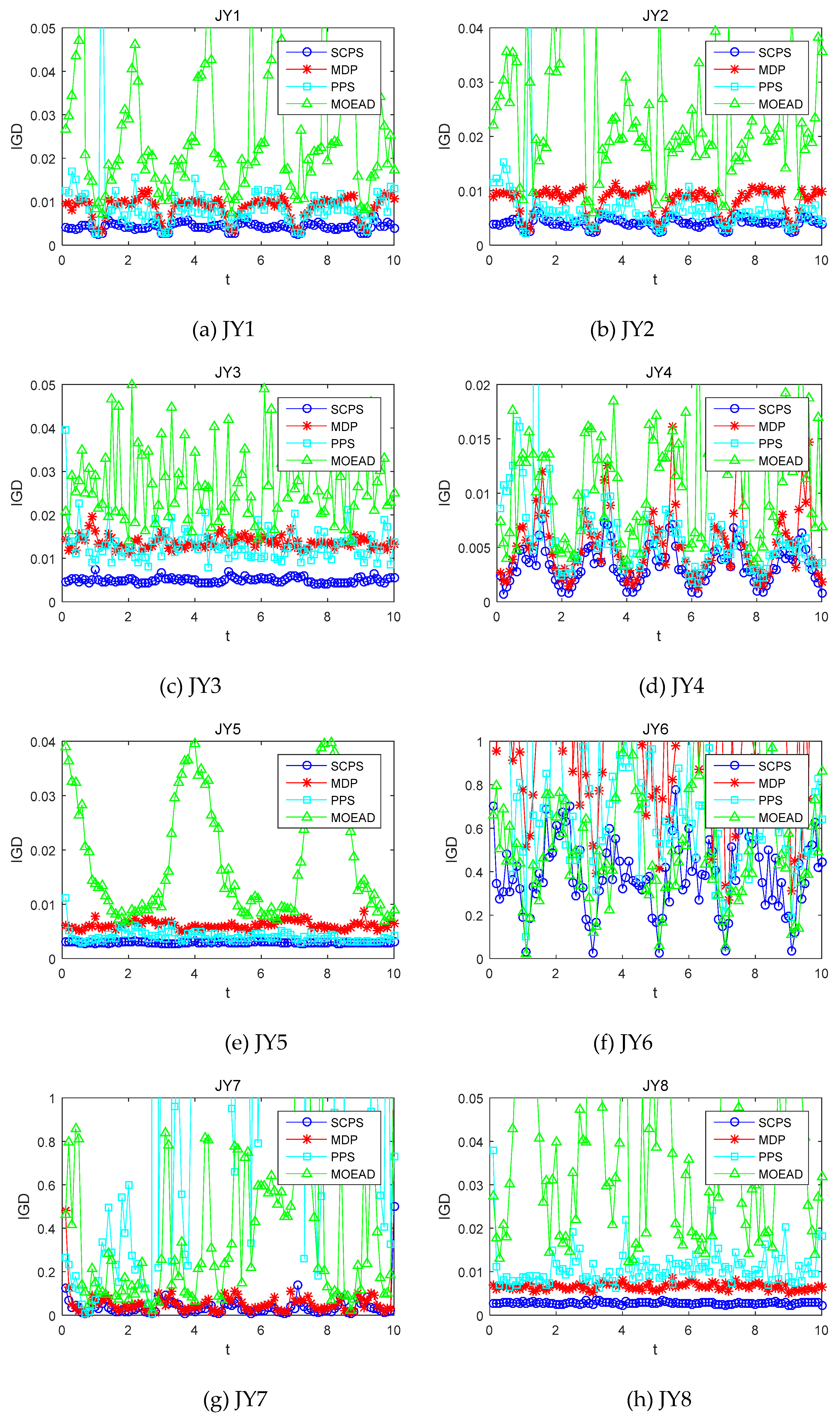
	10,20	2.77 × 10−3	2.06 × 10−5	6.72 × 10−3	1.19 × 10−4	7.57 × 10−3	1.93 × 10−3	4.21 × 10−2	1.47 × 10−3

shows the mean MIGD results of SCPS and other compared methods running 20 times in eight benchmark problems. The smaller the value of MIGD, the higher the average prediction accuracy. The optimal values are highlighted in bold.

SCPS has strong searching ability for the eight dynamic test problems. Only on the test problem JY4 ($(n,\tau )=(5,10)$), the PPS method is slightly better than the SCPS. For all the test problems, four algorithms have strong searching ability on JY1-JY5 as well as JY8. Their MIGDs reached the 10⁻² magnitude. That is, all these four algorithms have good ability to track the dynamic front.

JY6 is a Type III dynamic problem as shown in [25], where the multimodal PS and PD change over time, and the distribution of the optimal solution would be also in a constant process of change. Although the SCPS would be better than the other three algorithms on this problem, its MIGD is unsatisfactory.

JY7 is also a multimodal problem, and its PF shape is in a constant process of change. As the number of local optimum is fixed, JY7 is relatively simpler than JY6. Thus, the four algorithms running in JY7 are better than that in JY6. According to the standard deviation of MIGD, SCPS has better stability than the other 3 algorithms and a higher solution.

In order to analyze the dynamic searching ability of the four algorithms, eight group benchmark problems were chosen, and under the condition that $(n,\tau )=(10,20)$, the time-varying characteristic of IGD of algorithms was analyzed. Figure 3 shows the timely varying curves of IGD of the four algorithms running in the benchmark problem. Each time the environment changes, the smaller the IGD value is, and the more accurate the prediction of the algorithm.

It is indicted that the MOEA/D has a good searching performance in the static problem, but it could not dynamically predict. Thus, MOEA/D has an inadequate capability to solve the dynamic problem in bounded time. For the problems JY2 and JY5, PPS is better than MDP. However, for the problems JY7 and JY8, MDP is better than PPS. Especially, for JY7, large errors of the prediction might exist and keep increasing in PPS. In all eight benchmark problems, SCPS is better than the other three algorithms.

In order to further analyze the experimental results, the distribution of predicted results at five moments was compared for JY4, JY5, JY7, and JY8. Figure 4 shows the distribution of predicted results at five moments for the four algorithms running in four benchmark problems.

The discrete area of JY4 is time-varying. And the concavity of PF in JY5 changes over time. Although the PF changes of these two benchmark problems are different, they are both the unimodal problem. Thus, their results have good distribution and convergence. The PF shape of JY7 and JY8 would be changed all the time, so optimization is rather difficult. The points shown in Figure 4 are the non-dominant solution set of the population, and the number of these points reflects the performance of the algorithm. MDP and PPS have good distribution and convergence at the first moment, but the distribution of non-dominant solution set for these two algorithms is not satisfactory at the next four moments. That is, some points are far from the true PF. In comparison to the other three algorithms, SCPS performs particularly well in distribution and convergence. Moreover, in JY8, all four algorithms have good distribution, but SCPS performs better than the others in convergence.

According to the scatter distribution, SCPS has better searching performance. Its population segment provides an accurate shape change prediction. The cloud prediction strategy is the basic prediction strategy, and extra angle search is the main prediction angle error compensation.

Depending on the results of the IGD mean, IGD change with iterations, and scatter prediction results, the proposed algorithm is stable and has good predictive ability. Its prediction is more reasonable and closer to the population in the last moment.

5. Conclusions

The segment cloud prediction this paper proposed divides the population on the basis of the distance of PF. According to the results of center linear prediction for each population, the center position would be determined. Moreover, the population distribution is predicted by cloud theory. The angle error caused by the linear prediction process is decreased considerably by using extra angle search. The simulation results show that this algorithm has a better convergence and distribution, as well as environmental suitability. However, it cannot be denied that PF segmentation and cloud theory may not perform so well in the face of more difficult dynamic prediction problems, such as a mutation mapping relation between PF and PS. The high-dimensional dynamic multi-objective optimization problem is also an important research target, in which the effectiveness of Euclidean distance is also worth discussing. Future work can focus on these aspects.