The Inertial Sub-Gradient Extra-Gradient Method for a Class of Pseudo-Monotone Equilibrium Problems

Abstract

In this article, we focus on improving the sub-gradient extra-gradient method to find a solution to the problems of pseudo-monotone equilibrium in a real Hilbert space. The weak convergence of our method is well-established based on the standard assumptions on a bifunction. We also present the application of our results that enable to solve numerically the pseudo-monotone and monotone variational inequality problems, in addition to the particular presumptions required by the operator. We have used various numerical examples to support our well-proved convergence results, and we can show that the proposed method involves a considerable influence over-running time and the total number of iterations.

1. Introduction

Equilibrium problems involve many mathematical problems as a particular instance, such as minimization problems, complementarity problems, problems of fixed point, Non-cooperative games of Nash equilibrium problem, problems of saddle point and problem of vector minimization and the variational inequality problems (VIP) (for more details follow e.g., [1,2,3,4]). As an explanation of the equilibrium problem, we can also recognize this problem as a Ky Fan inequality, for the infer that Fan [5] produces research and proposes a specific condition on a bifunction for the presence of a solution of an equilibrium problem. As long as we know, Mu and Oettli [6] established this particular notion “equilibrium problem” in 1992 and was advanced further by Blum and Oettli [1]. Several authors have achieved and generalized many results with regard to the existence of an equilibrium problem solution (e.g., see [7,8,9,10,11] and the references therein). The development of new iterative methods and the examination of their converging analysis are among the most effective and valuable research directions in equilibrium theory. Several numerical results for solving the problem of equilibrium in different abstract spaces have been established (for instance, see [12,13,14,15,16,17,18,19,20,21,22,23,24,25,26,27]).

Two effective techniques are exceptionally well recognized due to their numerical efficiency i.e., the proximal point method [28] and the principle of auxiliary problem [29] are used to handle the problems of equilibrium. The proximal point method theory was basically formed by Martinet [30] in the case of the problem of monotone variational inequality and afterwards, this was enhanced by Rockafellar [31] in the case of monotone operators. Moudafi [28] provided the proximal point method for monotone equilibrium problems. This method is usually dealt with equilibrium problems that must contain a monotone bifunction. As a following, each sub-level problem is converted into a strong monotone equilibrium problem so that we can obtain its unique solution. However, in the case that the bifunction is a more general particular pseudo-monotone, we are not in a position to solve the equilibrium problem. Another important concept is the auxiliary problem principle, that is established on the understanding of forming a new problem that is analogous and generally simpler to carry out with respect to our initial problem. Cohen originally established this rule [32] for the problems of optimization, and further extended it to solve variational inequality problems [33]. Additionally, Mastroeni [29] introduced this theory in the case of problems of equilibrium engaged through strong monotone bifunction. On the other side, let us discuss inertial-type methods, which are based on said heavy ball methods of the second-order time dynamical system. In order to solve the problem of smooth convex minimization, Polyak [34] proposed an iterative scheme that would involve inertial extrapolation as a boost ingredient to the convergence of an iterative sequence. This approach is typically a two-step iterative scheme, and the next iteration is computed by taking the previous two iterations and can be referred to as a strategy of pacing up the iterative sequence ([34,35]). In the case of equilibrium problems, Moudafi initiated and proposed an inertial-type approach, specifically the second-order differential proximal method [36]. Such inertial methods are basically used to accelerate the iterative process to the desired solution. Numerical reviews suggest that inertial effects often improve the performance of the algorithm in terms of the number of iterations and time of execution in this context. There are many methods are already established for the different classes of variational inequality problem for more details see, [37,38,39,40,41].

In this study, we follow the Dadashi et al. sub-gradient extra-gradient method [42] and the method of Censor [43] and present their enhancement by implementing inertial technique. We are coming up with a modified sub-gradient extra-gradient method to solve problems of pseudo-monotone equilibrium in the setting of a real Hilbert space. The stepsize is not specified in our proposed method but is built up by an explicit formula based on some previous iterations. We are formulating a weak convergence theorem with regard to our recommended method of handling the problem of equilibriums under specific conditions. In addition, some application in the problem of variational inequality for monotone operator is considered and many numerical examples in finite and infinite dimensions are also taken in order to support the appropriateness of our proposed results.

The rest of this article will be structured according to the following: In Section 2, We are giving some concepts and relevant findings. Section 3, contains our algorithm involving pseudo-monotone bifunction, and provides the weak convergence result. Section 4, includes the application of our proposed results in variational inequality problems. Section 5, set out the numerical examples to demonstrate the algorithmic performance.

2. Preliminaries

Now we are including some of the important lemmas, definitions and other concepts that will be used throughout the convergence analysis. We were going to make use of that K as a closed, convex subset of the Hilbert space $\mathbb{E}.$ The notion $⟨.,.⟩$ and $\parallel .\parallel$ stands for the inner product and norm on the Hilbert space, receptively. We note down $u_n\rightharpoonup u^{*}$ to mention that the sequence $\left\{u_n\right\}$ weakly converges to $u^{*}.$ In addition, $EP(f,K)$ indicates the solution set of an (EP) on K and $u^{*}$ is an arbitrary element of $EP(f,K)$ or the solution set $VI(G,K)$ of a variational inequality problem G over C.

Definition 1.

[1] Let K to be a convex, closed and nonempty subset of $\mathbb{E}$ and $f:\mathbb{E}\times \mathbb{E}\to \mathbb{R}$ be a bifunction such that $f(u,u)=0$ for all $u\in K.$ The equilibrium problem respect to a bifunction f on K is reported in the following manner:

$$\mathit{find}{u}^{*}\in K\mathit{such}\mathit{that}f(u^{*},v)\ge 0,\mathit{for}\mathit{all}v\in K.$$

(EP)

Next, we consider certain notions of a bifunction monotonicity (see [1,44] for further information).

Definition 2.

The bifunction $f:\mathbb{E}\times \mathbb{E}\to \mathbb{R}$ on K for $\gamma >0$ is said to be:

(i) 

strongly monotone if $f(u,v)+f(v,u)\le {-\gamma \parallel u-v\parallel }^2,\forall u,v\in K;$

(ii) 

monotone if $f(u,v)+f(v,u)\le 0,\forall u,v\in K;$

(iii) 

strongly pseudo-monotone if $f(u,v)\ge 0⟹f(v,u)\le {-\gamma \parallel u-v\parallel }^2,\forall u,v\in K;$

(iv) 

pseudo-monotone if $f(u,v)\ge 0⟹f(v,u)\le 0,\forall u,v\in K;$

(v) 

satisfying the Lipschitz-type condition on K if there are two real numbers $L_1,L_2>0,$ such that

$$f(u,w)\le f(u,v)+f(v,w)+L_1{\parallel u-v\parallel }^2+L_2{\parallel v-w\parallel }^2,\forall u,v,w\in K.$$

Remark 1.

As a consequence, we have the following implications from the above definition.

$$\mathit{strongly}\mathit{monotone}⟹\mathit{monotone}⟹\mathit{pseudo}-\mathit{monotone}$$

$$\mathit{strongly}\mathit{monotone}⟹\mathit{strongly}\mathit{pseudo}-\mathit{monotone}⟹\mathit{pseudo}-\mathit{monotone}$$

Definition 3.

Assume $g:K\to \mathbb{R}$ is a convex function and subdifferential of g at $u\in K$ is define as follows:

$$\partial g\left(u\right)=\{z\in \mathbb{E}:g(v)-g(u)\ge ⟨z,v-u⟩,\forall v\in K\}.$$

Definition 4.

The normal cone of K at $u\in K$ is

$$N_K\left(u\right)=\{z\in \mathbb{E}:⟨z,v-u⟩\le 0,\forall v\in K\}.$$

Definition 5.

[45] A metric projection $P_K\left(u\right)$ of u onto a closed, convex subset K of $\mathbb{E}$ is define as

$$P_K\left(u\right)=\underset{v\in K}{argmin}\{\parallel v-u\parallel \}.$$

Lemma 1.

[46] Let $P_K:\mathbb{E}\to K$ be the metric projection from $\mathbb{E}$ onto $K.$ Thus, we have

(i) 

For all $u\in K,$ $v\in \mathbb{E},$

$$\parallel u-P_K{\left(v\right)\parallel }^2+\parallel P_K{\left(v\right)-v\parallel }^2\le {\parallel u-v\parallel }^2.$$

(ii) 

$w=P_K\left(u\right)$ if and only if

$$⟨u-w,v-w⟩\le 0.$$

This section ends with a few important lemmas that are useful in examining the convergence of our proposed results.

Lemma 2.

[47] Let K be a nonempty, closed and convex subset of a real Hilbert space $\mathbb{E}$ and $g:K\to \mathbb{R}$ be a convex, subdifferentiable with lower semicontinuous function on $K.$ Moreover, y is a minimizer of a function g if and only if $0\in \partial g\left(y\right)+N_K\left(y\right),$ where $\partial g\left(y\right)$ and $N_K\left(y\right)$ denotes the subdifferential of g at y and the normal cone of K at y respectively.

Lemma 3

([48], Page 31). For every $e,f\in \mathbb{E}$ and $\kappa \in \mathbb{R}$, then the following relation is true:

$${\parallel \kappa e+(1-\kappa )f\parallel }^2={\kappa \parallel e\parallel }^2+{(1-\kappa )\parallel f\parallel }^2-\kappa (1-\kappa ){\parallel e-f\parallel }^2.$$

Lemma 4.

[49] Let $a_n$, $b_n$ and $c_n$ are sequences in $[0,+\infty )$ such that

$$a_{n+1}\le a_n+b_n(a_n-a_{n-1})+c_n,\forall n\ge 1,\mathit{with}\sum _{n=1}^{+\infty }{c}_n<+\infty ,$$

while $b>0$ such that $0\le b_n\le b<1$ for all $n\in \mathbb{N}.$ Thus, the followings items are true:

$\left(i\right)$

${\sum }_{n=1}^{+\infty }{[a_n-a_{n-1}]}_{+}<\infty ,$ with ${\left[q\right]}_{+}:=max\{q,0\};$

$\left(ii\right)$

${lim}_{n\to +\infty }{a}_n=a^{*}\in [0,\infty ).$

Lemma 5.

[50] Let $\left\{{\eta }_n\right\}$ be a sequence in $\mathbb{E}$ and $K\subset \mathbb{E}$ such that

$\left(i\right)$

For each $\eta \in K,$ ${lim}_{n\to \infty }\parallel {\eta }_n-\eta \parallel$ exists;

$\left(ii\right)$

All sequentially weak cluster point of $\left\{{\eta }_n\right\}$ lies in K;

Then, $\left\{{\eta }_n\right\}$ weakly converges to a point in $K.$

Lemma 6.

[42] Assume $\left\{x_n\right\},\left\{y_n\right\}$ are sequences in $\mathbb{R}$ in such a way that $x_n\le y_n,$∀$n\in \mathbb{N}.$ Suppose that $\varrho ,\sigma \in (0,1)$ and $\mu \in (0,\sigma ).$ Then, there is a sequence ${\zeta }_n$ such that ${\zeta }_n{x}_n\le \mu y_n$ and ${\zeta }_n\in (\varrho \mu ,\sigma ).$

Due to Lipschitz-type condition on a bifunction f through above lemma, we have the subsequent inequality.

Corollary 1.

Assume f satisfy a Lipschitz-type condition on K through positive constants $L_1$ and $L_2.$ Let $\varrho \in (0,1),$ $\sigma <min\left\{\frac{1-3\vartheta }{{(1-\vartheta )}^2},\frac{1}{2L_1},\frac{1}{2L_2}\right\}$ where $\vartheta \in [0,\frac{1}{3})$ and $\mu \in (0,\sigma ).$ Then, there is a real number ζ such that

$$\zeta \left(f(u,w)-f(u,v)-L_1{\parallel u-v\parallel }^2-L_2{\parallel v-w\parallel }^2\right)\le \mu f(v,w),$$

and $\varrho \mu <\zeta <\sigma$ where $u,v,w\in K.$

Assumption 1.

Let a bifunction $f:\mathbb{E}\times \mathbb{E}\to \mathbb{R}$ satisfy the following conditions:

$f_1.$

$f(v,v)=0,$ for all $v\in K$ and f is pseudomontone on a set $K.$

$f_2.$

f satisfy the Lipschitz-type condition on $\mathbb{E}$ through positive constants $L_1$ and $L_2.$

$f_3.$

$\underset{n\to \infty }{lim\; sup}f(u_n,v)\le f(u^{*},v)$ for each $v\in K$ and $\left\{u_n\right\}\subset K$ satisfy $u_n\rightharpoonup u^{*}.$

$f_4.$

$f(u,.)$ need to be convex and subdifferentiable on K for arbitrary $u\in K.$

3. An Inertial Sub-Gradient Extra-Gradient Method and Its Convergence Analysis

Now we are presenting our first main algorithm and prove a weak convergence theorem to find a solution to the equilibrium problems (EP) involving pseudo-montone bifunction. The Algorithm 1 in details is given below.

Algorithm 1 Inertial sub-gradient extra-gradient method for pseudomontone (EP).

Initialization: Choose $u_{-1},u_0\in \mathbb{E},$ $\varrho \in (0,1),$ $\sigma <min\left\{\frac{1-3\vartheta }{{(1-\vartheta )}^2},\frac{1}{2c_1},\frac{1}{2c_2}\right\},$ $\mu \in (0,\sigma ),$ ${\zeta }_0>0$ and non-decreasing sequence $0\le {\vartheta }_n\le \vartheta \in [0,\frac{1}{3}).$ Set $$t_n=u_n+{\vartheta }_n(u_n-u_{n-1}).$$ Iterative steps: Given $u_{n-1},$ $u_n$ and ${\zeta }_n$ are known for $n\ge 0.$ Step 1: Find $$v_n=\underset{y\in K}{argmin}\{{\zeta }_{n}f(t_n,y)+\frac{1}{2}\parallel t_n-y{\parallel }^2\}.$$ If $t_n=v_n$; STOP. Otherwise, construct a half-space $${\Pi }_n=\{z\in \mathbb{E}:⟨t_n-{\zeta }_n{\omega }_n-v_n,z-v_n⟩\le 0\},$$ where ${\omega }_n\in {\partial }_{2}f(t_n,v_n).$ Step 2: Compute the next iterate $$u_{n+1}=\underset{y\in {\Pi }_n}{argmin}\{\mu {\zeta }_{n}f(v_n,y)+\frac{1}{2}\parallel t_n-y{\parallel }^2\}.$$ Next, the stepsize sequence ${\zeta }_{n+1}$ is updated as follows: $$\begin{array}{cc}\hfill {\zeta }_{n+1}=& min\left\{\sigma ,\frac{\mu f(v_n,u_{n+1})}{f(t_n,u_{n+1})-f(t_n,v_n)-c_1\parallel t_n-v_n{\parallel }^2-c_2{\parallel u_{n+1}-v_n\parallel }^2+1}\right\}\hfill \end{array}.$$ (1) Set $n:=n+1$ and go back to Iterative steps.

Remark 2.

By Corollary 1, ${\zeta }_{n+1}$ in Equation (1) is well-defined and

$${\zeta }_{n+1}\left(f(t_n,u_{n+1})-f(t_n,v_n)-c_1\parallel t_n-v_n{\parallel }^2-c_2{\parallel v_n-u_{n+1}\parallel }^2\right)\le \mu f(v_n,u_{n+1})$$

(2)

Now, we prove the validity of stopping criterion with regard to Algorithm 1.

Lemma 7.

If $v_n=t_n$ in Algorithm 1, then $t_n\in EP(f,K).$

Proof. 

By the definition of $v_n$ with Lemma 2, we have

$$0\in {\partial }_2\left\{{\zeta }_{n}f(t_n,y)+\frac{1}{2}{\parallel t_n-y\parallel }^2\right\}\left(v_n\right)+N_K\left(v_n\right).$$

Thus, there exists ${\omega }_n\in {\partial }_{2}f(t_n,v_n)$ and $\overline{\omega }\in N_K\left(v_n\right)$ so that ${\zeta }_n{\omega }_n+v_n-t_n+\overline{\omega }=0.$ Due to hypothesis $t_n=v_n$ implies that ${\zeta }_n{\omega }_n+\overline{\omega }=0.$ Thus, we have

$${\zeta }_n⟨{\omega }_n,y-v_n⟩+⟨\overline{\omega },y-v_n⟩=0,\forall y\in K.$$

By $\overline{\omega }\in N_K\left(v_n\right)$ implies $⟨\overline{\omega },y-v_n⟩\le 0$ and through above expression, we obtain

$${\zeta }_n⟨{\omega }_n,y-v_n⟩\ge 0,\forall y\in K.$$

(3)

By ${\omega }_n\in f(t_n,v_n)$ and the subdifferential definition, we obtain

$$f(t_n,y)-f(t_n,v_n)\ge ⟨w_n,y-v_n⟩,\forall y\in K.$$

(4)

By Equations (3) and (4) with ${\zeta }_n\in (0,+\infty )$ implies that $f(t_n,y)\ge 0$ for all $y\in K.$ □

Lemma 8.

Let bifunction $f:\mathbb{E}\times \mathbb{E}\to \mathbb{R}$ follows the conditions ($f_1$-$f_4$). Thus, for each $u^{*}\in EP(f,K)\ne \varnothing ,$ we could have

$$\begin{array}{cc}\hfill \parallel u_{n+1}-u^{*}{\parallel }^2& \le \parallel t_n-u^{*}{\parallel }^2-(1-{\zeta }_{n+1}){\parallel u_{n+1}-t_n\parallel }^2\hfill \\ \hfill & -{\zeta }_{n+1}(1-2c_1{\zeta }_n)\parallel t_n-v_n{\parallel }^2-{\zeta }_{n+1}(1-2c_2{\zeta }_n){\parallel u_{n+1}-v_n\parallel }^2.\hfill \end{array}$$

Proof. 

By Lemma 2 with definition of $u_{n+1},$ we have

$$0\in {\partial }_2\left\{\mu {\zeta }_{n}f(v_n,y)+\frac{1}{2}{\parallel t_n-y\parallel }^2\right\}\left(u_{n+1}\right)+N_{{\Pi }_n}\left(u_{n+1}\right).$$

From above implies that $\omega \in {\partial }_{2}f(v_n,u_{n+1})$ and $\overline{\omega }\in N_{{\Pi }_n}\left(u_{n+1}\right)$ such that

$$\mu {\zeta }_n\omega +u_{n+1}-t_n+\overline{\omega }=0.$$

Thus, we have

$$⟨t_n-u_{n+1},y-u_{n+1}⟩=\mu {\zeta }_n⟨\omega ,y-u_{n+1}⟩+⟨\overline{\omega },y-u_{n+1}⟩,\forall y\in {\Pi }_n.$$

Since $\overline{\omega }\in N_{{\Pi }_n}\left(u_{n+1}\right)$ then $⟨\overline{\omega },y-u_{n+1}⟩\le 0$ for all $y\in {\Pi }_n.$ This gives

$$\mu {\zeta }_n⟨\omega ,y-u_{n+1}⟩\ge ⟨t_n-u_{n+1},y-u_{n+1}⟩,\forall y\in {\Pi }_n.$$

(5)

By $\omega \in {\partial }_{2}f(v_n,u_{n+1}),$ we can obtain

$$f(v_n,y)-f(v_n,u_{n+1})\ge ⟨\omega ,y-u_{n+1}⟩,\forall y\in K.$$

(6)

Combining expression (5) and (6), we get

$$\mu {\zeta }_{n}f(v_n,y)-\mu {\zeta }_{n}f(v_n,u_{n+1})\ge ⟨t_n-u_{n+1},y-u_{n+1}⟩,\forall y\in K.$$

(7)

By substituting $y=u^{*}$ into expression (7), we get

$$\mu {\zeta }_{n}f(v_n,u^{*})-\mu {\zeta }_{n}f(v_n,u_{n+1})\ge ⟨t_n-u_{n+1},u^{*}-u_{n+1}⟩,\forall y\in K.$$

(8)

Since $u^{*}\in EP(f,K)$ then implies that $f(u^{*},v_n)\ge 0$ and due to the pseudomonotonicity of a bifunction f we can get $f(v_n,u^{*})\le 0.$ Therefore, from (8), we get

$$⟨t_n-u_{n+1},u_{n+1}-u^{*}⟩\ge \mu {\zeta }_{n}f(v_n,u_{n+1}).$$

(9)

By the expression (2) and (9) implies that

$$\begin{array}{cc}\hfill ⟨t_n-u_{n+1},u_{n+1}-u^{*}⟩\ge & {\zeta }_{n+1}[{\zeta }_n\left\{f(t_n,u_{n+1})-f(t_n,v_n)\right\}\hfill \\ \hfill & -c_1{\zeta }_n\parallel t_n-v_n{\parallel }^2-c_2{\zeta }_n{\parallel u_{n+1}-v_n\parallel }^2].\hfill \end{array}$$

(10)

Since $u_{n+1}\in {\Pi }_n$ and then by the definition of ${\Pi }_n$ implies that $⟨t_n-{\zeta }_n{\omega }_n-v_n,u_{n+1}-v_n⟩\le 0.$ Thus, we have

$${\zeta }_n⟨{\omega }_n,u_{n+1}-v_n⟩\ge ⟨t_n-v_n,u_{n+1}-v_n⟩.$$

(11)

Since ${\omega }_n\in {\partial }_{2}f(t_n,v_n)$ with $y=u_{n+1},$ we gain

$$f(t_n,u_{n+1})-f(t_n,v_n)\ge ⟨{\omega }_n,u_{n+1}-v_n⟩,\forall y\in K.$$

(12)

By combining (11) and (12), we have

$${\zeta }_n\left\{f(t_n,u_{n+1})-f(t_n,v_n)\right\}\ge ⟨t_n-v_n,u_{n+1}-v_n⟩.$$

(13)

Next, combining (10) and (13), we get

$$\begin{array}{cc}\hfill 2⟨t_n-u_{n+1},u_{n+1}-u^{*}⟩& \ge {\zeta }_{n+1}[2⟨t_n-v_n,u_{n+1}-v_n⟩\hfill \\ \hfill & -2c_1{\zeta }_n\parallel t_n-v_n{\parallel }^2-2c_2{\zeta }_n{\parallel u_{n+1}-v_n\parallel }^2].\hfill \end{array}$$

(14)

We have the following facts:

$$2⟨t_n-u_{n+1},u_{n+1}-u^{*}⟩=\parallel t_n-u^{*}{\parallel }^2-\parallel u_{n+1}-t_n{\parallel }^2-{\parallel u_{n+1}-u^{*}\parallel }^2.$$

$$2⟨t_n-v_n,u_{n+1}-v_n⟩=\parallel t_n-v_n{\parallel }^2+\parallel u_{n+1}-v_n{\parallel }^2-{\parallel t_n-u_{n+1}\parallel }^2.$$

From the above last two inequalities and Equation (14), we obtain

$$\begin{array}{cc}\hfill \parallel u_{n+1}-u^{*}{\parallel }^2& \le \parallel t_n-u^{*}{\parallel }^2-(1-{\zeta }_{n+1}){\parallel u_{n+1}-t_n\parallel }^2\hfill \\ \hfill & -{\zeta }_{n+1}(1-2c_1{\zeta }_n)\parallel t_n-v_n{\parallel }^2-{\zeta }_{n+1}(1-2c_2{\zeta }_n){\parallel u_{n+1}-v_n\parallel }^2.\hfill \end{array}$$

□

Theorem 1.

Let a bifunction $f:\mathbb{E}\times \mathbb{E}\to \mathbb{R}$ satisfying the assumptions ($f_1$-$f_4$). Thus, for each $u^{*}\in EP(f,K)\ne \varnothing ,$ the sequence $\left\{t_n\right\},$ $\left\{u_n\right\}$ and $\left\{v_n\right\}$ generated by Algorithm 1, converges weakly to $u^{*}.$

Proof. 

By Lemma 8, we write

$$\begin{array}{cc}\hfill \parallel u_{n+1}-u^{*}{\parallel }^2& \le \parallel t_n-u^{*}{\parallel }^2-(1-{\zeta }_{n+1}){\parallel u_{n+1}-t_n\parallel }^2\hfill \\ \hfill & -{\zeta }_{n+1}(1-2c_1{\zeta }_n)\parallel t_n-v_n{\parallel }^2-{\zeta }_{n+1}(1-2c_2{\zeta }_n){\parallel u_{n+1}-v_n\parallel }^2.\hfill \end{array}$$

(15)

Thus, for $n\ge 1$ above expression implies that

$$\begin{array}{cc}\hfill \parallel u_{n+1}-u^{*}{\parallel }^2& \le \parallel t_n-u^{*}{\parallel }^2-(1-{\zeta }_{n+1}){\parallel u_{n+1}-t_n\parallel }^2.\hfill \end{array}$$

(16)

By $t_n$ in Algorithm 1, we get

$$\begin{array}{cc}\parallel t_n-u^{*}{\parallel }^2\hfill & =\parallel u_n+{\vartheta }_n(u_n-u_{n-1})-u^{*}{\parallel }^2\hfill \\ \hfill & =\parallel (1+{\vartheta }_n)(u_n-u^{*})-{\vartheta }_n(u_{n-1}-u^{*}){\parallel }^2\hfill \\ \hfill & =(1+{\vartheta }_n)\parallel u_n-u^{*}{\parallel }^2-{\vartheta }_n\parallel u_{n-1}-u^{*}{\parallel }^2+{\vartheta }_n(1+{\vartheta }_n){\parallel u_n-u_{n-1}\parallel }^2.\hfill \end{array}$$

(17)

Furthermore, by the definition $t_n$ and follows the Cauchy inequality, we have

$$\begin{array}{}& \hfill \parallel u_{n+1}-t_n{\parallel }^2& =\parallel u_{n+1}-u_n-{\vartheta }_n(u_n-u_{n-1}){\parallel }^2\hfill \mathrm{(18)}& & =\parallel u_{n+1}-u_n{\parallel }^2+{\vartheta }_n^2{\parallel u_n-u_{n-1}\parallel }^2-2{\vartheta }_n⟨u_{n+1}-u_n,u_n-u_{n-1}⟩\hfill & & \ge \parallel u_{n+1}-u_n{\parallel }^2+{\vartheta }_n^2\parallel u_n-u_{n-1}{\parallel }^2-2{\vartheta }_n\parallel u_{n+1}-u_n\parallel \parallel u_n-u_{n-1}\parallel \hfill & & \ge \parallel u_{n+1}-u_n{\parallel }^2+{\vartheta }_n^2\parallel u_n-u_{n-1}{\parallel }^2-{\vartheta }_n\parallel u_{n+1}-u_n{\parallel }^2-{\vartheta }_n{\parallel u_n-u_{n-1}\parallel }^2\hfill \mathrm{(19)}& & \ge (1-{\vartheta }_n)\parallel u_{n+1}-u_n{\parallel }^2+({\vartheta }_n^2-{\vartheta }_n){\parallel u_n-u_{n-1}\parallel }^2.\hfill \end{array}$$

By combining the expression (16), (17) and (19), we are getting

$$\begin{array}{}& \parallel u_{n+1}-u^{*}{\parallel }^2& \le (1+{\vartheta }_n)\parallel u_n-u^{*}{\parallel }^2-{\vartheta }_n\parallel u_{n-1}-u^{*}{\parallel }^2+{\vartheta }_n(1+{\vartheta }_n){\parallel u_n-u_{n-1}\parallel }^2\mathrm{(20)}& -(1-{\zeta }_{n+1})\left[(1-{\vartheta }_n)\parallel u_{n+1}-u_n{\parallel }^2+({\vartheta }_n^2-{\vartheta }_n){\parallel u_n-u_{n-1}\parallel }^2\right]& \le (1+{\vartheta }_n)\parallel u_n-u^{*}{\parallel }^2-{\vartheta }_n\parallel u_{n-1}-u^{*}{\parallel }^2-(1-{\zeta }_{n+1})(1-{\vartheta }_n){\parallel u_{n+1}-u_n\parallel }^2& +\left[{\vartheta }_n(1+{\vartheta }_n)-(1-{\zeta }_{n+1})({\vartheta }_n^2-{\vartheta }_n)\right]{\parallel u_n-u_{n-1}\parallel }^2\mathrm{(21)}& \le (1+{\vartheta }_n)\parallel u_n-u^{*}{\parallel }^2-{\vartheta }_n\parallel u_{n-1}-u^{*}{\parallel }^2-Q_n\parallel u_{n+1}-u_n{\parallel }^2+R_n{\parallel u_n-u_{n-1}\parallel }^2,\end{array}$$

where

$$Q_n=(1-{\zeta }_{n+1})(1-{\vartheta }_n),$$

and

$$R_n={\vartheta }_n(1+{\vartheta }_n)-(1-{\zeta }_{n+1})({\vartheta }_n^2-{\vartheta }_n).$$

Further, we put

$${\mathsf{\Phi }}_n=\parallel u_n-u^{*}{\parallel }^2-{\vartheta }_n\parallel u_{n-1}-u^{*}{\parallel }^2+R_n{\parallel u_n-u_{n-1}\parallel }^2.$$

Next, we compute

$$\begin{array}{cc}\hfill {\mathsf{\Phi }}_{n+1}-{\mathsf{\Phi }}_n& =\parallel u_{n+1}-u^{*}{\parallel }^2-{\vartheta }_{n+1}\parallel u_n-u^{*}{\parallel }^2+R_{n+1}{\parallel u_{n+1}-u_n\parallel }^2\hfill \\ \hfill & -\parallel u_n-u^{*}{\parallel }^2+{\vartheta }_n\parallel u_{n-1}-u^{*}{\parallel }^2-R_n{\parallel u_n-u_{n-1}\parallel }^2\hfill \\ \hfill & =\parallel u_{n+1}-u^{*}{\parallel }^2-(1+{\vartheta }_{n+1})\parallel u_n-u^{*}{\parallel }^2+{\vartheta }_n{\parallel u_{n-1}-u^{*}\parallel }^2\hfill \\ \hfill & +R_{n+1}\parallel u_{n+1}-u_n{\parallel }^2-R_n{\parallel u_n-u_{n-1}\parallel }^2\hfill \\ \hfill & \le \parallel u_{n+1}-u^{*}{\parallel }^2-(1+{\vartheta }_n)\parallel u_n-u^{*}{\parallel }^2+{\vartheta }_n{\parallel u_{n-1}-u^{*}\parallel }^2\hfill \\ \hfill & +R_{n+1}\parallel u_{n+1}-u_n{\parallel }^2-R_n{\parallel u_n-u_{n-1}\parallel }^2\hfill \\ \hfill & \le -(Q_n-R_{n+1}){\parallel u_{n+1}-u_n\parallel }^2.\hfill \end{array}$$

(22)

We obtain the above last inequality from Equation (21) and

$$\begin{array}{cc}\hfill & Q_n-R_{n+1}\hfill \\ \hfill & =(1-{\zeta }_{n+1})(1-{\vartheta }_n)-{\vartheta }_{n+1}(1+{\vartheta }_{n+1})+(1-{\zeta }_{n+2})({\vartheta }_{n+1}^2-{\vartheta }_{n+1})\hfill \\ \hfill & \ge (1-\sigma ){(1-{\vartheta }_{n+1})}^2-{\vartheta }_{n+1}-{\vartheta }_{n+1}^2\hfill \\ \hfill & \ge (1-\sigma ){(1-\vartheta )}^2-\vartheta -{\vartheta }^2\hfill \\ \hfill & ={(1-\vartheta )}^2-\sigma {(1-\vartheta )}^2-\vartheta -{\vartheta }^2\hfill \\ \hfill & =(1-3\vartheta )-\sigma {(1-\vartheta )}^2\hfill \\ \hfill \end{array}$$

(23)

By our hypothesis and for some $\delta >0,$ we get

$${\mathsf{\Phi }}_{n+1}-{\mathsf{\Phi }}_n\le -(Q_n-R_{n+1})\parallel u_{n+1}-u_n{\parallel }^2\le -\delta {\parallel u_{n+1}-u_n\parallel }^2.$$

(24)

So the above implies that $\left\{{\mathsf{\Phi }}_n\right\}$ is non-increasing. From the definition of ${\mathsf{\Phi }}_{n+1},$ we have

$$\begin{array}{cc}\hfill {\mathsf{\Phi }}_{n+1}& =\parallel u_{n+1}-u^{*}{\parallel }^2-{\vartheta }_{n+1}\parallel u_n-u^{*}{\parallel }^2+R_{n+1}{\parallel u_{n+1}-u_n\parallel }^2\hfill \\ \hfill & \ge -{\vartheta }_{n+1}{\parallel u_n-u^{*}\parallel }^2.\hfill \end{array}$$

(25)

In addition, from ${\mathsf{\Phi }}_n$ we have

$$\begin{array}{cc}\hfill {\mathsf{\Phi }}_n& =\parallel u_n-u^{*}{\parallel }^2-{\vartheta }_n\parallel u_{n-1}-u^{*}{\parallel }^2+R_n{\parallel u_n-u_{n-1}\parallel }^2\hfill \\ \hfill & \ge \parallel u_n-u^{*}{\parallel }^2-{\vartheta }_n{\parallel u_{n-1}-u^{*}\parallel }^2.\hfill \end{array}$$

(26)

The above implies that

$$\begin{array}{cc}\hfill \parallel u_n-u^{*}{\parallel }^2& \le {\mathsf{\Phi }}_n+{\vartheta }_n{\parallel u_{n-1}-u^{*}\parallel }^2\hfill \\ \hfill & \le {\mathsf{\Phi }}_1+\vartheta {\parallel u_{n-1}-u^{*}\parallel }^2\hfill \\ \hfill & \le {\mathsf{\Phi }}_1+\vartheta \left[{\mathsf{\Phi }}_1+\vartheta {\parallel u_{n-2}-u^{*}\parallel }^2\right]\hfill \\ \hfill & \le {\mathsf{\Phi }}_1+\vartheta {\mathsf{\Phi }}_1+{\vartheta }^2{\parallel u_{n-2}-u^{*}\parallel }^2\hfill \\ \hfill & \le \cdots \le {\mathsf{\Phi }}_1({\vartheta }^{n-1}+\cdots +1)+{\vartheta }^n{\parallel u_0-u^{*}\parallel }^2\hfill \\ \hfill & \le \frac{{\mathsf{\Phi }}_1}{1-\vartheta }+{\vartheta }^n{\parallel u_0-u^{*}\parallel }^2.\hfill \end{array}$$

(27)

Combining (25) and (27) we obtain

$$\begin{array}{cc}\hfill -{\mathsf{\Phi }}_{n+1}& \le {\vartheta }_{n+1}{\parallel u_n-u^{*}\parallel }^2\hfill \\ \hfill & \le \vartheta \parallel u_n-u^{*}{\parallel }^2\hfill \\ \hfill & \le \vartheta \frac{{\mathsf{\Phi }}_1}{1-\vartheta }+{\vartheta }^{n+1}{\parallel u_0-u^{*}\parallel }^2.\hfill \end{array}$$

(28)

It follow from the expression (24) and (28) that

$$\begin{array}{cc}\hfill \delta \sum _{n=1}^k\parallel u_{n+1}-u_n\parallel & \le {\mathsf{\Phi }}_1-{\mathsf{\Phi }}_{k+1}\hfill \\ \hfill & \le {\mathsf{\Phi }}_1+\vartheta \frac{{\mathsf{\Phi }}_1}{1-\vartheta }+{\vartheta }^{k+1}{\parallel u_0-u^{*}\parallel }^2\hfill \\ \hfill & \le \frac{{\mathsf{\Phi }}_1}{1-\vartheta }+{\parallel u_0-u^{*}\parallel }^2.\hfill \end{array}$$

(29)

letting $k\to \infty$ in above expression implies that

$$\sum _{n=1}^{\infty }\parallel u_{n+1}-u_n\parallel <+\infty ⟹\underset{n\to \infty }{lim}\parallel u_{n+1}-u_n\parallel =0.$$

(30)

From (18) and (30) we can obtain

$$\parallel u_{n+1}-t_n\parallel \to 0\mathrm{as}n\to \infty .$$

(31)

By expression (20) with Lemma 4 and ${\sum }_{n=1}^{\infty }\parallel u_{n+1}-u_n\parallel <+\infty$ implies that

$$\underset{n\to \infty }{lim}{\parallel u_n-u^{*}\parallel }^2=l,\mathrm{for}\mathrm{some}\mathrm{finite}l>0.$$

(32)

By (17), (30) and (32) we also get

$$\underset{n\to \infty }{lim}{\parallel t_n-u^{*}\parallel }^2=l.$$

(33)

Next, we show that ${lim}_{n\to \infty }{\parallel v_n-u^{*}\parallel }^2=l.$ It follows from Lemma 8, for $n\ge 1$ such that

$$\begin{array}{cc}\hfill & {\zeta }_{n+1}(1-2c_1{\zeta }_n){\parallel t_n-v_n\parallel }^2\hfill \\ \hfill & \le \parallel t_n-u^{*}{\parallel }^2-{\parallel u_{n+1}-u^{*}\parallel }^2\hfill \\ \hfill & \le (\parallel t_n-u^{*}\parallel +\parallel u_{n+1}-u^{*}\parallel \left)\right(\parallel t_n-u^{*}\parallel -\parallel u_{n+1}-u^{*}\parallel )\hfill \\ \hfill & \le (\parallel t_n-u^{*}\parallel +\parallel u_{n+1}-u^{*}\parallel )\parallel u_{n+1}-t_n\parallel ⟶0\mathrm{as}n\to \infty .\hfill \end{array}$$

(34)

The above implies that

$$\underset{n\to \infty }{lim}\parallel t_n-v_n\parallel =0.$$

(35)

The above expression with (33) gives that

$$\underset{n\to \infty }{lim}{\parallel v_n-u^{*}\parallel }^2=l.$$

(36)

It follows from (31) and (35) such that

$$0\le \parallel u_{n+1}-v_n\parallel =\parallel u_{n+1}-t_n\parallel +\parallel t_n-v_n\parallel ⟶0\mathrm{as}n\to \infty .$$

(37)

The above implies that for each $u^{*}\in EP(f,K),$ the ${lim}_{n\to \infty }{\parallel u_n-u^{*}\parallel }^2$ exists and also the sequences $\left\{u_n\right\}$, $\left\{t_n\right\}$ and $\left\{v_n\right\}$ are bounded. Now, we prove that all weak cluster point respect to the sequence $\left\{u_n\right\}$ lies inside in $EP(f,K).$ For this we take z is any weak cluster point of $\left\{u_n\right\}$, i.e., there is a subsequence, indicated by $\left\{u_{n_k}\right\}$, of $\left\{u_n\right\}$ converges weakly to $z.$ Due to $\parallel u_n-v_n\parallel \to 0$ implies that $\left\{v_{n_k}\right\}$ too converges weakly to z and $z\in K.$ Let prove that $z\in EP(f,K).$ By the expression (7), (2) and (13), we have

$$\begin{array}{cc}\hfill \mu {\zeta }_{n}f(v_n,y)& \ge \mu {\zeta }_{n}f(v_{n_k},u_{n_k+1})+⟨t_{n_k}-u_{n_k+1},y-u_{n_k+1}⟩\hfill \\ \hfill & \ge {\zeta }_n{\zeta }_{n+1}f(t_{n_k},u_{n_{k+1}})-{\zeta }_n{\zeta }_{n+1}f(t_{n_k},v_{n_k})-c_1{\zeta }_n{\zeta }_{n+1}{\parallel t_{n_k}-v_{n_k}\parallel }^2\hfill \\ \hfill & -c_2{\zeta }_n{\zeta }_{n+1}{\parallel v_{n_k}-u_{n_k+1}\parallel }^2+⟨t_{n_k}-u_{n_k+1},y-u_{n_k+1}⟩\hfill \\ \hfill & \ge {\zeta }_{n+1}⟨t_{n_k}-v_{n_k},u_{n_k+1}-v_{n_k}⟩-c_1{\zeta }_n{\zeta }_{n+1}{\parallel t_{n_k}-v_{n_k}\parallel }^2\hfill \\ \hfill & -c_2{\zeta }_n{\zeta }_{n+1}{\parallel v_{n_k}-u_{n_k+1}\parallel }^2+⟨t_{n_k}-u_{n_k+1},y-u_{n_k+1}⟩\hfill \end{array}$$

(38)

for any element $y\in K.$ Moreover, from (31), (35), (37) and the boundness of $\left\{u_n\right\}$ implies that right-hand side of above inequity appears may to zero as $n\to \infty$. Using $\mu ,{\zeta }_n>0,$ condition ($f_3$) in (Assumption 1) and $v_{n_k}\rightharpoonup z,$ we have

$$0\le \underset{k\to \infty }{lim\; sup}f(v_{n_k},y)\le f(z,y),\mathrm{for}\mathrm{all}y\in K.$$

(39)

Given that $z\in K$ and $f(z,y)\ge 0$, for all $y\in K.$ It gives that $z\in EP(f,K).$ Finally, we establish that the sequence $\left\{u_n\right\}$ converges weakly to $u^{*}$ by using the Lemma 5. This completes the proof. □

If we use ${\vartheta }_n=0$ in the Algorithm 1, we get an algorithm that appears in the Dadashi et al. [42].

Corollary 2.

Let a bifunction $f:\mathbb{E}\times \mathbb{E}\to \mathbb{R}$ satisfying the assumptions ($f_1$–$f_4$). Thus, for every $u^{*}\in EP(f,K)\ne \varnothing ,$ the sequence $\left\{u_n\right\}$ and $\left\{v_n\right\}$ are generated as follows:

i. 

Given $u_0\in \mathbb{E},$ $\varrho \in (0,1),$ $\sigma <min\{1,\frac{1}{2c_1},\frac{1}{2c_2}\},$ $\mu \in (0,\sigma )$ and ${\zeta }_0>0.$

ii. 

Compute

$$\left\{\begin{array}{c}{v}_n=\underset{y\in K}{argmin}\{{\zeta }_{n}f(u_n,y)+\frac{1}{2}\parallel u_n-y{\parallel }^2\},\hfill \\ u_{n+1}=\underset{y\in {\Pi }_n}{argmin}\{\mu {\zeta }_{n}f(v_n,y)+\frac{1}{2}\parallel u_n-y{\parallel }^2\},\hfill \end{array}\right.$$

with ${\Pi }_n=\{z\in \mathbb{E}:⟨u_n-{\zeta }_n{\omega }_n-v_n,z-v_n⟩\le 0\}$ where ${\omega }_n\in {\partial }_{2}f(u_n,v_n).$ Moreover, the stepsize sequence ${\zeta }_{n+1}$ is updated as follows:

$$\begin{array}{cc}\hfill {\zeta }_{n+1}=& min\left\{\sigma ,\frac{\mu f(v_n,u_{n+1})}{f(u_n,u_{n+1})-f(u_n,v_n)-c_1\parallel u_n-v_n{\parallel }^2-c_2{\parallel u_{n+1}-v_n\parallel }^2+1}\right\}.\hfill \end{array}$$

The sequence $\left\{u_n\right\}$ and $\left\{v_n\right\}$ weakly converges to the solution $u^{*}\in EP(f,K).$

4. Solution for Variational Inequality Problems

We state the variational inequality problem as follows:

$$\mathrm{Find}{u}^{*}\in K\mathrm{such}\mathrm{that}⟨G\left(u^{*}\right),v-u^{*}⟩\ge 0,\forall v\in K.$$

A operator $G:\mathbb{E}\to \mathbb{E}$ is called

• monotone on K if $⟨G\left(u\right)-G\left(v\right),u-v⟩\ge 0,\forall u,v\in K;$
• pseudo-monotone on K if $⟨G\left(u\right),v-u⟩\ge 0\Rightarrow ⟨G\left(v\right),u-v⟩\le 0,\forall u,v\in K;$
• L-Lipschitz continuous on K if $\parallel G\left(u\right)-G\left(v\right)\parallel \le L\parallel u-v\parallel ,\forall u,v\in K.$

Note: if we take the bifunction $f(u,v):=⟨G\left(u\right),v-u⟩$ for all $u,v\in K,$ then the equilibrium problem convert into the above variational inequality problem with $L=2L_1=2L_2.$ By definitions of $v_n$ in the Algorithm 1 and the above definition of bifunction f such that

$$\begin{array}{cc}\hfill v_n& =\underset{y\in K}{argmin}\left\{{\zeta }_{n}f(t_n,y)+\frac{1}{2}{\parallel t_n-y\parallel }^2\right\}\hfill \\ \hfill & =\underset{y\in K}{argmin}\left\{{\zeta }_n⟨G\left(t_n\right),y-t_n⟩+\frac{1}{2}\parallel t_n{-y\parallel }^2+\frac{{\zeta }_n^2}{2}{\parallel G\left(t_n\right)\parallel }^2\right\}\hfill \\ \hfill & =\underset{y\in K}{argmin}\left\{\frac{1}{2}{\parallel t_n-{\zeta }_{n}G\left(t_n\right)-y\parallel }^2\right\}\hfill \\ \hfill & =P_K(t_n-{\zeta }_{n}G\left(t_n\right)).\hfill \end{array}$$

(40)

Due to ${\omega }_n\in {\partial }_{2}f(t_n,v_n)$ and by subdifferential definition, we obtain

$$\begin{array}{cc}\hfill ⟨{\omega }_n,z-v_n⟩& \le ⟨G\left(t_n\right),z-t_n⟩-⟨G\left(t_n\right),v_n-t_n⟩,\forall z\in \mathbb{E}\hfill \\ \hfill & =⟨G\left(t_n\right),z-v_n⟩,\forall z\in \mathbb{E},\hfill \end{array}$$

(41)

and consequently $0\le ⟨G\left(t_n\right)-{\omega }_n,z-v_n⟩.$ That is why we have

$$\begin{array}{cc}\hfill & ⟨t_n-{\zeta }_{n}G\left(t_n\right)-v_n,z-v_n⟩\hfill \\ \hfill & \le ⟨t_n-{\zeta }_{n}G\left(t_n\right)-v_n,z-v_n⟩+{\zeta }_n⟨G\left(t_n\right)-{\omega }_n,z-v_n⟩\hfill \\ \hfill & \le ⟨t_n-{\zeta }_n{\omega }_n-v_n,z-v_n⟩.\hfill \end{array}$$

(42)

Similarly to the expression (40), $u_{n+1}$ in Algorithm 1 convert into

$$u_{n+1}=P_{{\Pi }_n}(t_n-\mu {\zeta }_{n}G\left(v_n\right)).$$

Assumption 2.

Suppose that G satisfying the following assumptions:

$G_1^{*}$.

G is monotone on K and $VI(G,K)$ is nonempty;

$G_1$.

G is pseudo-monotone on K and $VI(G,K)$ is nonempty;

$G_2$.

G is L-Lipschitz continuous on K for constant $L>0.$

$G_3$.

$\underset{n\to \infty }{lim\; sup}⟨G\left(u_n\right),v-u_n⟩\le ⟨G\left(u^{*}\right),v-u^{*}⟩$ for every $v\in K$ and $\left\{u_n\right\}\subset K$ satisfying $u_n\rightharpoonup u^{*}.$

As a result, the inertial sub-gradient extra-gradient Algorithm 1 with Theorem 1 covert to the subsequent result for solving the variational inequality problems.

Corollary 3.

Assume that $G:K\to \mathbb{E}$ is satisfying ($G_1,G_2,G_3$) as in Assumption 2. Let $\left\{t_n\right\},$ $\left\{u_n\right\}$ and $\left\{v_n\right\}$ be the sequences generated as follows:

i. 

Choose $u_{-1},u_0\in \mathbb{E},$ $\varrho \in (0,1),$ $\sigma <min\left\{\frac{1-3\vartheta }{{(1-\vartheta )}^2},\frac{1}{L}\right\},$ $\mu \in (0,\sigma ),$ ${\zeta }_0>0$ and non-decreasing sequence $0\le {\vartheta }_n\le \vartheta \in [0,\frac{1}{3}).$

ii. 

Given $u_{n-1},u_n$ and compute

$$\left\{\begin{array}{c}{v}_n=P_K(t_n-{\zeta }_{n}G\left(t_n\right)),\mathit{where}{t}_n=u_n+{\vartheta }_n(u_n-u_{-1}),\hfill \\ u_{n+1}=P_{{\Pi }_n}(t_n-\mu {\zeta }_{n}G\left(v_n\right)),\hfill \end{array}\right.$$

where ${\Pi }_n=\{z\in \mathbb{E}:⟨t_n-{\zeta }_{n}G\left(t_n\right)-v_n,z-v_n⟩\le 0\}.$ Moreover, the stepsize sequence ${\zeta }_{n+1}$ is updated as follows:

$$\begin{array}{cc}\hfill {\zeta }_{n+1}=& min\left\{\sigma ,\frac{\mu ⟨G{v}_n,u_{n+1}-v_n⟩}{⟨G{t}_n,u_{n+1}-v_n⟩-\frac{L}{2}\parallel t_n-v_n{\parallel }^2-\frac{L}{2}{\parallel u_{n+1}-v_n\parallel }^2+1}\right\}.\hfill \end{array}$$

The sequence $\left\{t_n\right\},$ $\left\{u_n\right\}$ and $\left\{v_n\right\}$ weakly converges to the solution $u^{*}$ of $VI(G,K).$

Corollary 4.

Assume that $G:K\to \mathbb{E}$ is satisfying ($G_1,G_2,G_3$) as in Assumption 2. Let $\left\{u_n\right\}$ and $\left\{v_n\right\}$ be the sequences generated as follows:

i. 

Choose $u_0\in \mathbb{E},$ $\varrho \in (0,1),$ $\sigma <min\left\{1,\frac{1}{L}\right\},$ $\mu \in (0,\sigma )$ and ${\zeta }_0>0.$

ii. 

Given $u_n$ and compute

$$\left\{\begin{array}{c}{v}_n=P_K(u_n-{\zeta }_{n}G\left(u_n\right)),\hfill \\ u_{n+1}=P_{{\Pi }_n}(u_n-\mu {\zeta }_{n}G\left(v_n\right)),\hfill \end{array}\right.$$

where ${\Pi }_n=\{z\in \mathbb{E}:⟨u_n-{\zeta }_{n}G\left(u_n\right)-v_n,z-v_n⟩\le 0\}.$ Moreover, the stepsize sequence ${\zeta }_{n+1}$ is updated as follows:

$$\begin{array}{cc}\hfill {\zeta }_{n+1}=& min\left\{\sigma ,\frac{\mu ⟨G{v}_n,u_{n+1}-v_n⟩}{⟨G{u}_n,u_{n+1}-v_n⟩-\frac{L}{2}\parallel u_n-v_n{\parallel }^2-\frac{L}{2}{\parallel u_{n+1}-v_n\parallel }^2+1}\right\}.\hfill \end{array}$$

The sequence $\left\{u_n\right\}$ and $\left\{v_n\right\}$ weakly converges to the solution $u^{*}$ of $VI(G,K).$

Next, we consider that provided G is monotone, assumption ($G_3$) can be removed. The assumption ($G_3$) is needed to express $f(u,v)=⟨G\left(u\right),v-u⟩$ satisfy the assumption ($f_3$). In addition, condition ($f_3$) is used to prove $z\in EP(f,K)$, see description (39). This means that condition ($G_3$) is employed to show $z\in VI(G,K).$ Next, we are continuing to show $z\in VI(G,K)$ by applying the monotonicity of operator $G.$ This means that

$$⟨G\left(v\right),v-v_n⟩\ge ⟨G\left(v_n\right),v-v_n⟩,\forall v\in K.$$

(43)

By $f(u,v)=⟨G\left(u\right),v-u⟩$ and expression (38), we get

$$\underset{k\to \infty }{lim\; sup}⟨G\left(v_{n_k}\right),v-v_{n_k}⟩\ge 0,\forall v\in K.$$

(44)

Combining (43) with (44), we conclude that

$$\underset{k\to \infty }{lim\; sup}⟨G\left(v\right),v-v_{n_k}⟩\ge 0,\forall v\in K.$$

(45)

Therefore $v_{n_k}\rightharpoonup z\in K,$ implies that $⟨G\left(v\right),v-z⟩\ge 0,$∀$v\in K.$ Let $v_t=(1-t)z+tv$ for all $t\in [0,1].$ Due to the convexity of K, $v_t\in K$ for each $t\in (0,1).$ Then, we can write

$$0\le ⟨G\left(v_t\right),v_t-z⟩=t⟨G\left(v_t\right),v-z⟩$$

(46)

That is $⟨G\left(v_t\right),v-z⟩\ge 0$ for every $t\in (0,1).$ From $v_t\to z$ as $t\to 0$ and the continuity of $G,$ we reach $⟨G\left(z\right),v-z⟩\ge 0$ for all $v\in K,$ this shows that $z\in VI(G,K).$

Corollary 5.

Assume that $G:K\to \mathbb{E}$ is satisfying ($G_1^{*},G_2$) as in Assumption 2. Let $\left\{t_n\right\},$ $\left\{u_n\right\}$ and $\left\{v_n\right\}$ are sequences created as follows:

i. 

Take $u_{-1},u_0\in \mathbb{E},$ $\varrho \in (0,1),$ $\sigma <min\left\{\frac{1-3\vartheta }{{(1-\vartheta )}^2},\frac{1}{L}\right\},$ $\mu \in (0,\sigma ),$ ${\zeta }_0>0$ and non-decreasing sequence $0\le {\vartheta }_n\le \vartheta \in [0,\frac{1}{3}).$

ii. 

Given $u_{n-1},u_n$ and compute

$$\left\{\begin{array}{c}{v}_n=P_K(t_n-{\zeta }_{n}G\left(t_n\right)),\mathit{where}{t}_n=u_n+{\vartheta }_n(u_n-u_{-1}),\hfill \\ u_{n+1}=P_{{\Pi }_n}(t_n-\mu {\zeta }_{n}G\left(v_n\right)),\hfill \end{array}\right.$$

where ${\Pi }_n=\{z\in \mathbb{E}:⟨t_n-{\zeta }_{n}G\left(t_n\right)-v_n,z-v_n⟩\le 0\}.$ Moreover, the stepsize sequence ${\zeta }_{n+1}$ is updated as follows:

$$\begin{array}{cc}\hfill {\zeta }_{n+1}=& min\left\{\sigma ,\frac{\mu ⟨G{v}_n,u_{n+1}-v_n⟩}{⟨G{t}_n,u_{n+1}-v_n⟩-\frac{L}{2}\parallel t_n-v_n{\parallel }^2-\frac{L}{2}{\parallel u_{n+1}-v_n\parallel }^2+1}\right\}.\hfill \end{array}$$

Then, the sequence $\left\{t_n\right\},$ $\left\{u_n\right\}$ and $\left\{v_n\right\}$ weakly converges to the solution $u^{*}$ of $VI(G,K).$

Corollary 6.

Assume that $G:K\to \mathbb{E}$ is satisfying ($G_1^{*},G_2$) as in Assumption 2. Let $\left\{u_n\right\}$ and $\left\{v_n\right\}$ be the sequences generated as follows:

i. 

Choose $u_0\in \mathbb{E},$ $\varrho \in (0,1),$ $\sigma <min\left\{1,\frac{1}{L}\right\},$ $\mu \in (0,\sigma )$ and ${\zeta }_0>0.$

ii. 

Given $u_n$ and compute

$$\left\{\begin{array}{c}{v}_n=P_K(u_n-{\zeta }_{n}G\left(u_n\right)),\hfill \\ u_{n+1}=P_{{\Pi }_n}(u_n-\mu {\zeta }_{n}G\left(v_n\right)),\hfill \end{array}\right.$$

where ${\Pi }_n=\{z\in \mathbb{E}:⟨u_n-{\zeta }_{n}G\left(u_n\right)-v_n,z-v_n⟩\le 0\}.$ Moreover, the stepsize sequence ${\zeta }_{n+1}$ is updated as follows:

$$\begin{array}{cc}\hfill {\zeta }_{n+1}=& min\left\{\sigma ,\frac{\mu ⟨G{v}_n,u_{n+1}-v_n⟩}{⟨G{u}_n,u_{n+1}-v_n⟩-\frac{L}{2}\parallel u_n-v_n{\parallel }^2-\frac{L}{2}{\parallel u_{n+1}-v_n\parallel }^2+1}\right\}.\hfill \end{array}$$

Then, the sequence $\left\{u_n\right\}$ and $\left\{v_n\right\}$ weakly converges to the solution $u^{*}$ of $VI(G,K).$

5. Computational Experiment

Some numerical results will be presented to show the efficiency of our above-mentioned methods. The MATLAB codes run in MATLAB version 9.5 (R2018b) on a PC Intel(R) Core(TM)i5-6200 CPU @ 2.30 GHz 2.40 GHz, RAM 8.00 GB. During all these examples we use $u_0=v_0={(1,1,\cdots ,1,1)}^T$ and y-axes display error term $D_n$ while the x-axis refers to the total number of iterations or the running time (in seconds). Moreover, for our proposed Algorithm 1 (Shortly, Int.EgA) with error term $D_n=\parallel t_n-v_n\parallel$ and for Tran et al. [23] (Shortly, Tran.EgA) and Dadashi et al. [42] (Shortly, Dadshi.EgA) with error term $D_n=\parallel u_n-v_n\parallel .$

5.1. Example 1

Suppose that there will be n firms which generates the same product. Let u stands for a vector in which the each entry $u_i$ denote the amount of the product manufactured by the firm i. We take the price P as a decreasing affine function that depends upon on the value of $S={\sum }_{i=1}^m{u}_i$ i.e., $P_i\left(S\right)={\varphi }_i-{\psi }_{i}S,$ where ${\varphi }_i>0,$ ${\psi }_i>0.$ The profit function for each firm i is define by $F_i\left(u\right)=P_i\left(S\right)u_i-t_i\left(u_i\right),$ where $t_i\left(u_i\right)$ is tax and producing cost $u_i.$ Assume $K_i=[u_i^{min},u_i^{max}]$ is set of strategies belongs to each firm $i,$ and the strategy scheme for the whole model take the form as $K:=K_1\times K_2\times \cdots \times K_n.$ In fact, each firm aims to achieve its maximum revenue by taking the corresponding level of growth on the assumption that production of the other companies is an input parameter. The technique often utilized to deal such type of model focuses mainly on the well-known Nash equilibrium concept. We would like to remind that point $u^{*}\in K=K_1\times K_2\times \cdots \times K_n$ is the point of equilibrium of the model if

$$F_i\left(u^{*}\right)\ge F_i\left(u^{*}\left[u_i\right]\right)\forall u_i\in K_i,\forall i=1,2,\cdots ,n.$$

with the vector $u^{*}\left[u_i\right]$ represent the vector get from $u^{*}$ by taking $u_i^{*}$ with $u_i.$ Finally, we take $f(u,v):=\phi (u,v)-\phi (u,u)$ with $\phi (u,v):=-{\sum }_{i=1}^n{F}_i\left(u\left[v_i\right]\right),$ and the problem of evaluating the Nash equilibrium point as:

$$\mathrm{find}{u}^{*}\in K:f(u^{*},v)\ge 0,\forall v\in K.$$

In addition, we assume that both the tax and the fee for the production of the unit are increasing as the amount of productivity increases. It follows from [18,23], the function f could be taken in the following:

$$f(u,v)=⟨Pu+Qv+q,v-u⟩,$$

where $q\in {\mathbb{R}}^n$ and P, Q are matrices of order n so that $Q-P$ is symmetric negative definite and Q is symmetric positive semidefinite with Lipschitz constants $L_1=L_2=\frac{1}{2}\parallel P-Q\parallel$ (for more details see, [23]). During this Example in Section 5.1, the matrices $P,Q$ are generated randomly (Two matrices A, B are randomly generated with entries from $[-1,1].$ The matrix $Q=A^{T}A,$ $S=B^{T}B$ and $P=S+Q$). and entries of q randomly belongs to $[-1,1].$ The feasible set $K\subset {\mathbb{R}}^n$ is written as

$$K:=\{u\in {\mathbb{R}}^n:-5\le u_i\le 5\}.$$

The experimental results are shown in Figure 1, Figure 2, Figure 3 and Figure 4 and Table 1 with $\zeta =\frac{1}{4L_1},$ $\sigma =\frac{5}{11L_1},$ $\mu =\frac{5}{12L_1},$ ${\vartheta }_n=\frac{1}{4}$ and ${\zeta }_0=\frac{1}{4L_1}.$

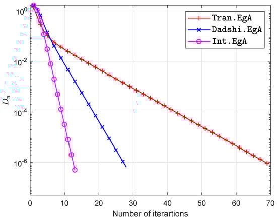
Figure 1. Example in Section 5.1 when $n=5$.

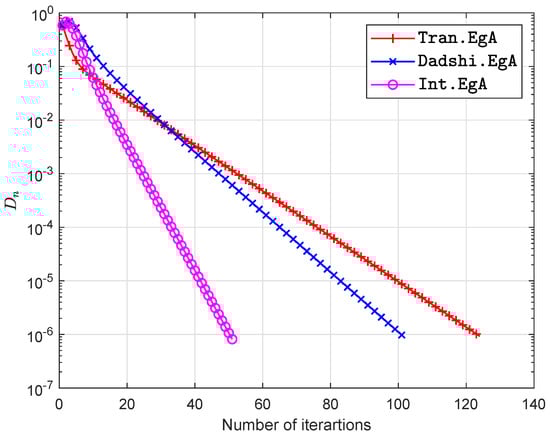
Figure 2. Example in Section 5.1 when $n=10$.

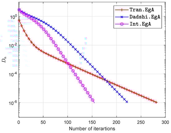
Figure 3. Example in Section 5.1 when $n=20$.

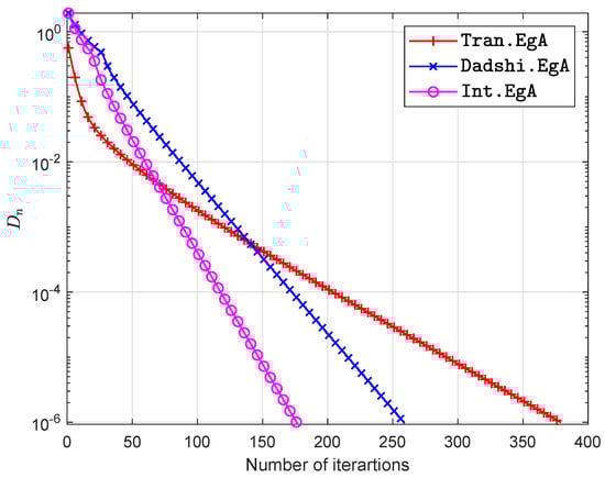
Figure 4. Example in Section 5.1 when $n=40$.

Table 1. The experimental finding for Figure 1, Figure 2, Figure 3 and Figure 4.

	Tran.EgA		Dadshi.EgA		Int.EgA
n	Iter.	CPU(s)	Iter.	CPU(s)	Iter.	CPU(s)
5	69	0.5508	28	0.2356	13	0.1145
10	124	1.2234	101	0.8967	51	0.4338
20	283	3.4558	223	2.5063	155	1.4874
40	379	5.1930	259	3.0970	177	1.7652

5.2. Example 2

Let take $G:{\mathbb{R}}^2\to {\mathbb{R}}^2$ be explained by

$$F\left(x\right)=\left(\begin{array}{c}0.5u_1{u}_2-2u_2-{10}^7\\ -4u_1-0.1u_2^2-{10}^7\end{array}\right)$$

and let $K=\{u\in {\mathbb{R}}^2:{(u_1-2)}^2+{(u_2-2)}^2\le 1\}.$ It is east to see F is Lipschitz continuous with $L=5$ and pseudo-monotone. During these experiments we use stepsize $\zeta ={10}^{-8}$ for Tran et al. [23] and ${\zeta }_0=0.1$, $\sigma =0.199,$ ${\vartheta }_n=0.25$ and $\mu =0.19.$ The experimental results are shown in Table 2 and Figure 5, Figure 6, Figure 7 and Figure 8.

Table 2. Results for Figure 5, Figure 6, Figure 7 and Figure 8.

	Tran.EgA		Dadshi.EgA		Int.EgA
u0 = v0	Iter.	CPU(s)	Iter.	CPU(s)	Iter.	CPU(s)
$(1.5,1.7)$	86	2.9587	62	1.9962	40	1.6405
$(2.0,3.0)$	89	3.5329	71	2.0817	46	1.4633
$(1.0,2.0)$	99	3.4713	73	2.2057	52	1.5730
$(2.7,2.6)$	71	2.7353	55	1.9161	36	1.2266

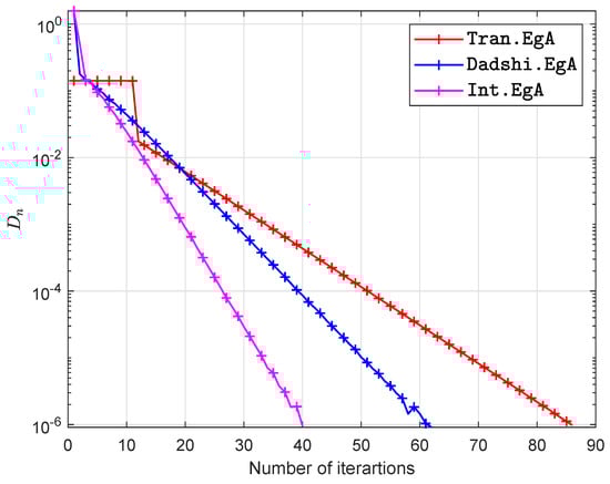
Figure 5. Example in Section 5.2 when $u_0=v_0=(1.5,1.7)$.

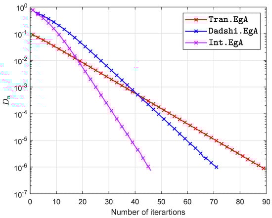
Figure 6. Example in Section 5.2 when $u_0=v_0=(2.0,3.0)$.

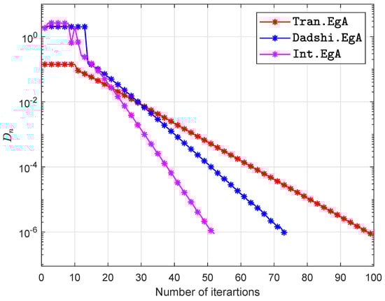
Figure 7. Example in Section 5.2 when $u_0=v_0=(1.0,2.0)$.

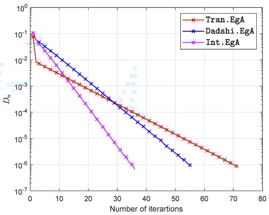
Figure 8. Example in Section 5.2 when $u_0=v_0=(2.7,2.6)$.

5.3. Example 3

Let a bifunction f define on the convex set K as

$$f(u,v)=⟨(B{B}^T+S+D)u,v-u⟩$$

where B is an order n matrix, S is an order n skew-symmetric matrix, D is an order n diagonal matrix, having nonnegative entries. The feasible set $K\subset {\mathbb{R}}^m$ defined as

$$K=\{u\in {\mathbb{R}}^m:Au\le b\},$$

while A is $l\times m$ matrix and b is nonnegative vector. We can see that bifunction is monotone with Lipschitz-type constants are $L_1=L_2=\frac{\parallel B{B}^T+S+D\parallel }{2}.$ The numerical findings shall be noted in Figure 9, Figure 10 and Figure 11 and Table 3 with $\zeta =\frac{1}{4L_1},$ $\sigma =\frac{5}{11L_1},$ $\mu =\frac{5}{12L_1},$ ${\vartheta }_n=\frac{1}{4}$ and ${\zeta }_0=\frac{1}{4L_1}.$

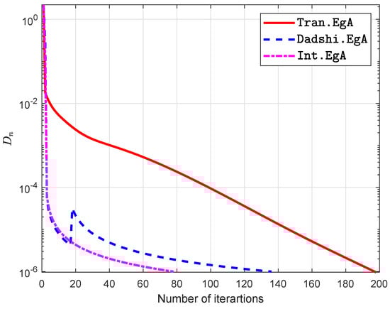
Figure 9. Example in Section 5.3 when $n=5$.

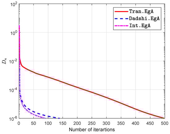
Figure 10. Example in Section 5.3 when $n=10$.

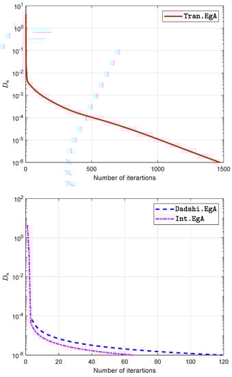
Figure 11. Example in Section 5.3 when $n=20$.

Table 3. The numerical results for Figure 9, Figure 10 and Figure 11.

	Tran.EgA		Dadshi.EgA		Int.EgA
u0 = v0	Iter.	CPU(s)	Iter.	CPU(s)	Iter.	CPU(s)
5	198	4.6833	136	2.0156	78	1.1475
10	498	13.9149	190	2.3003	94	0.8930
20	1471	35.1972	119	1.5241	65	0.8603

5.4. Example 4

Let $\mathbb{E}=l_2$ be the real Hilbert space having elements are square-summable infinite sequence of real numbers and $K=\{u\in \mathbb{E}:\parallel u\parallel \le 3\}.$ Let a bifunction $f(u,v)=(5-\parallel u\parallel )⟨u,v-u⟩\forall u,v\in \mathbb{E},$ where $\parallel u\parallel =\sqrt{{\sum }_i{\left|u_i\right|}^2}.$ We can easily check that $EP(f,K)\ne \varnothing$ and also satisfy the assumption ${\iota }_3.$ Next, we show that bifunction is Lipschitz-type continuous

$$\begin{array}{cc}\hfill & f(u,w)-f(u,v)-f(v,w)\hfill \\ \hfill & =(5-\parallel u\parallel )⟨u,w-u⟩-(5-\parallel u\parallel )⟨u,v-u⟩-(5-\parallel v\parallel )⟨v,w-v⟩\hfill \\ \hfill & =(5-\parallel u\parallel )⟨u,w-v⟩-(5-\parallel v\parallel )⟨v,w-v⟩\hfill \\ \hfill & =⟨(5-\parallel u\parallel )u-(5-\parallel v\parallel )v,w-v⟩\hfill \\ \hfill & \le \parallel (5-\parallel u\parallel )u-(5-\parallel v\parallel )v\parallel \parallel v-w\parallel \hfill \\ \hfill & =\parallel 5(u-v)-\parallel u\parallel (u-v)-(\parallel u\parallel -\parallel v\parallel )v\parallel \parallel v-w\parallel \hfill \\ \hfill & \le \left[5\parallel u-v\parallel +\parallel u\parallel \parallel u-v\parallel +|\parallel u\parallel -\parallel v\parallel |\parallel v\parallel \right]\parallel v-w\parallel \hfill \\ \hfill & \le \left[5\parallel u-v\parallel +3\parallel u-v\parallel +3\parallel u-v\parallel \right]\parallel v-w\parallel \hfill \\ \hfill & =11\parallel u-v\parallel \parallel v-w\parallel \hfill \\ \hfill & \le \frac{11}{2}{\parallel u-v\parallel }^2+\frac{11}{2}{\parallel v-w\parallel }^2,\hfill \end{array}$$

while $u,v,w\in K$ and value of Lipschitz-constants are $L_1=L_2=\frac{11}{2}.$ Next, we prove that bifunction is pseudo-monotone. Let $u,v\in K$ be so that $f(u,v)=(5-\parallel u\parallel )⟨u,v-u⟩\ge 0,$ mean that $⟨u,v-u⟩\ge 0.$ Thus

$$\begin{array}{cc}\hfill f(v,u)& =(5-\parallel v\parallel )⟨v,u-v⟩\hfill \\ \hfill & \le (5-\parallel v\parallel )⟨v,u-v⟩+(5-\parallel v\parallel )⟨u,v-u⟩\hfill \\ \hfill & \le (5-\parallel v\parallel )⟨v,u-v⟩-(5-\parallel v\parallel )⟨u,u-v⟩\hfill \\ \hfill & \le {(\parallel v\parallel -5)\parallel u-v\parallel }^2\le 0.\hfill \end{array}$$

Next, we show that bifunction f is not monotone. Let we take $u=(\frac{5}{2},0,0,\cdots ,0,\cdots )$ and $v=(3,0,0,\cdots ,0,\cdots )$ in a manner that

$$\begin{array}{cc}\hfill f(u,v)+f(v,u)& =\frac{5}{2}⟨u,v-u⟩+2⟨v,u-v⟩>0.\hfill \end{array}$$

The projection onto K is explicitly computed as

$$P_K\left(u\right)=\left\{\begin{array}{c}u\mathrm{if}\parallel u\parallel \le 3,\hfill \\ \frac{3u}{\parallel u\parallel },\mathrm{otherwise}.\hfill \end{array}\right.$$

The numerical results are shown in Figure 12 and Figure 13 and Table 4 with $\zeta =\frac{1}{4L_1},$ $\sigma =\frac{5}{11L_1},$ $\mu =\frac{5}{12L_1},$ ${\vartheta }_n=\frac{1}{4}$ and ${\zeta }_0=\frac{1}{4L_1}.$

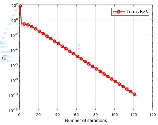
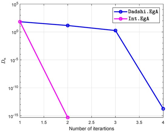
Figure 12. Example in Section 5.4 when $u_0=v_0=(1,1,\cdots ,1_{5000},0,0,\cdots )$.

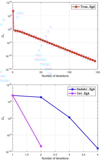
Figure 13. Example in Section 5.4 when $u_0=v_0=(1,1,\cdots ,1_{5000},0,0,\cdots )$.

Table 4. The numerical results for Figure 12 and Figure 13.

	Tran.EgA		Dadshi.EgA		Int.EgA
u0 = v0	Iter.	CPU(s)	Iter.	CPU(s)	Iter.	CPU(s)
$(1,1,\cdots ,1_{5000},0,0,\cdots )$	69	0.5508	28	0.2356	13	0.1145
$(1,2,\cdots ,5000,0,0,\cdots )$	124	1.2234	101	0.8967	51	0.4338

6. Conclusions

We have provided an extra-gradient-like method to resolve pseudo-monotone equilibrium problems in real Hilbert space. The key influence of our recommended method is that our generated iterative sequences have been integrated with the particular step-size evaluation formula. The stepsize formula is revised for each iteration based on the preceding iterations. Numerical conclusions were performed in order to explain our algorithm’s numerical performance contrasted with other methods. Such numerical reviews prove that inertial effects often normally promote the performance of the iterative sequence in this context.

References

- Blum, E. From optimization and variational inequalities to equilibrium problems. Math. Stud. 1994, 63, 123–145. [Google Scholar]
- Facchinei, F.; Pang, J.S. Finite-Dimensional Variational Inequalities and Complementarity Problems; Springer Science & Business Media: New York, NY, USA, 2007. [Google Scholar]
- Konnov, I. Equilibrium Models and Variational Inequalities; Elsevier: New York, NY, USA, 2007; Volume 210. [Google Scholar]
- Giannessi, F.; Maugeri, A.; Pardalos, P.M. Equilibrium Problems: Nonsmooth Optimization and Variational Inequality Models; Springer Science & Business Media: New York, NY, USA, 2006; Volume 58. [Google Scholar]
- Fan, K. A Minimax Inequality and Applications, Inequalities III; Shisha, O., Ed.; Academic Press: New York, NY, USA, 1972. [Google Scholar]
- Muu, L.D.; Oettli, W. Convergence of an adaptive penalty scheme for finding constrained equilibria. Nonlinear Anal. Theory, Methods Appl. 1992, 18, 1159–1166. [Google Scholar] [CrossRef]
- Yuan, G.X.Z. KKM Theory and Applications in Nonlinear Analysis; CRC Press: New York, NY, USA, 1999; Volume 218. [Google Scholar]
- Brézis, H.; Nirenberg, L.; Stampacchia, G. A remark on Ky Fan’s minimax principle. Bollettino dell Unione Matematica Italiana 2008, 1, 257–264. [Google Scholar]
- Ansari, Q.; Wong, N.C.; Yao, J.C. The existence of nonlinear inequalities. Appl. Math. Lett. 1999, 12, 89–92. [Google Scholar] [CrossRef]
- Rehman, H.U.; Kumam, P.; Sompong, D. Existence of tripled fixed points and solution of functional integral equations through a measure of noncompactness. Carpathian J. Math. 2019, 35, 193–208. [Google Scholar]
- Rehman, H.U.; Gopal, G.; Kumam, P. Generalizations of Darbo’s fixed point theorem for new condensing operators with application to a functional integral equation. Demonstr. Math. 2019, 52, 166–182. [Google Scholar] [CrossRef]
- Antipin, A.S. The convergence of proximal methods to fixed points of extremal mappings and estimates of their rate of convergence. Comput. Math. Math. Phys. 1995, 35, 539–552. [Google Scholar]
- Combettes, P.L.; Hirstoaga, S.A. Equilibrium programming in Hilbert spaces. J. Nonlinear Convex Anal. 2005, 6, 117–136. [Google Scholar]
- Flåm, S.D.; Antipin, A.S. Equilibrium programming using proximal-like algorithms. Math. Program. 1996, 78, 29–41. [Google Scholar] [CrossRef]
- Van Hieu, D.; Muu, L.D.; Anh, P.K. Parallel hybrid extragradient methods for pseudomonotone equilibrium problems and nonexpansive mappings. Numer. Algorithms 2016, 73, 197–217. [Google Scholar] [CrossRef]
- Van Hieu, D.; Anh, P.K.; Muu, L.D. Modified hybrid projection methods for finding common solutions to variational inequality problems. Comput. Optim. Appl. 2017, 66, 75–96. [Google Scholar] [CrossRef]
- Van Hieu, D. Halpern subgradient extragradient method extended to equilibrium problems. Revista de la Real Academia de Ciencias Exactas Físicas y Naturales Ser. A Matemáticas 2017, 111, 823–840. [Google Scholar] [CrossRef]
- Hieua, D.V. Parallel extragradient-proximal methods for split equilibrium problems. Math. Model. Anal. 2016, 21, 478–501. [Google Scholar] [CrossRef]
- Konnov, I. Application of the proximal point method to nonmonotone equilibrium problems. J. Optim. Theory Appl. 2003, 119, 317–333. [Google Scholar] [CrossRef]
- Iusem, A.N.; Sosa, W. Iterative algorithms for equilibrium problems. Optimization 2003, 52, 301–316. [Google Scholar] [CrossRef]
- Quoc, T.D.; Anh, P.N.; Muu, L.D. Dual extragradient algorithms extended to equilibrium problems. J. Glob. Optim. 2012, 52, 139–159. [Google Scholar] [CrossRef]
- ur Rehman, H.; Kumam, P.; Cho, Y.J.; Yordsorn, P. Weak convergence of explicit extragradient algorithms for solving equilibirum problems. J. Inequalities Appl. 2019, 2019, 1–25. [Google Scholar] [CrossRef]
- Quoc Tran, D.; Le Dung, M.; Nguyen, V.H. Extragradient algorithms extended to equilibrium problems. Optimization 2008, 57, 749–776. [Google Scholar] [CrossRef]
- Santos, P.; Scheimberg, S. An inexact subgradient algorithm for equilibrium problems. Comput. Appl. Math. 2011, 30, 91–107. [Google Scholar]
- Takahashi, S.; Takahashi, W. Viscosity approximation methods for equilibrium problems and fixed point problems in Hilbert spaces. J. Math. Anal. Appl. 2007, 331, 506–515. [Google Scholar] [CrossRef]
- Rehman, H.U.; Kumam, P.; Abubakar, A.B.; Cho, Y.J. The extragradient algorithm with inertial effects extended to equilibrium problems. Comput. Appl. Math. 2020, 39, 1–26. [Google Scholar]
- Rehman, H.U.; Kumam, P.; Cho, Y.J.; Suleiman, Y.I.; Kumam, W. Modified Popov’s explicit iterative algorithms for solving pseudomonotone equilibrium problems. Optim. Methods. Softw. 2020, 0, 1–32. [Google Scholar]
- Moudafi, A. Proximal point algorithm extended to equilibrium problems. J. Nat. Geom. 1999, 15, 91–100. [Google Scholar]
- Mastroeni, G. On auxiliary principle for equilibrium problems. In Equilibrium Problems and Variational Models; Springer: Berlin, Germany, 2003; pp. 289–298. [Google Scholar]
- Martinet, B. Brève communication. Régularisation d’inéquations variationnelles par approximations successives. Revue Française D’informatique et De recherche Opérationnelle. Série Rouge 1970, 4, 154–158. [Google Scholar] [CrossRef]
- Rockafellar, R.T. Monotone operators and the proximal point algorithm. SIAM J. Control. Optim. 1976, 14, 877–898. [Google Scholar] [CrossRef]
- Cohen, G. Auxiliary problem principle and decomposition of optimization problems. J. Optim. Theory Appl. 1980, 32, 277–305. [Google Scholar] [CrossRef]
- Cohen, G. Auxiliary problem principle extended to variational inequalities. J. Optim. Theory Appl. 1988, 59, 325–333. [Google Scholar] [CrossRef]
- Polyak, B.T. Some methods of speeding up the convergence of iteration methods. USSR Comput. Math. Math. Phys. 1964, 4, 1–17. [Google Scholar] [CrossRef]
- Beck, A.; Teboulle, M. A fast iterative shrinkage-thresholding algorithm for linear inverse problems. SIAM J. Imaging Sci. 2009, 2, 183–202. [Google Scholar] [CrossRef]
- Moudafi, A. Second-order differential proximal methods for equilibrium problems. J. Inequalities Pure Appl. Math. 2003, 4, 1–7. [Google Scholar]
- Dong, Q.L.; Lu, Y.Y.; Yang, J. The extragradient algorithm with inertial effects for solving the variational inequality. Optimization 2016, 65, 2217–2226. [Google Scholar] [CrossRef]
- Thong, D.V.; Van Hieu, D. Modified subgradient extragradient method for variational inequality problems. Numer. Algorithms 2018, 79, 597–610. [Google Scholar] [CrossRef]
- Dong, Q.; Cho, Y.; Zhong, L.; Rassias, T.M. Inertial projection and contraction algorithms for variational inequalities. J. Glob. Optim. 2018, 70, 687–704. [Google Scholar] [CrossRef]
- Yang, J. Self-adaptive inertial subgradient extragradient algorithm for solving pseudomonotone variational inequalities. Appl. Anal. 2019. [Google Scholar] [CrossRef]
- Thong, D.V.; Van Hieu, D.; Rassias, T.M. Self adaptive inertial subgradient extragradient algorithms for solving pseudomonotone variational inequality problems. Optim. Lett. 2020, 14, 115–144. [Google Scholar] [CrossRef]
- Dadashi, V.; Iyiola, O.S.; Shehu, Y. The subgradient extragradient method for pseudomonotone equilibrium problems. Optimization 2019, 1–23. [Google Scholar] [CrossRef]
- Censor, Y.; Gibali, A.; Reich, S. The subgradient extragradient method for solving variational inequalities in Hilbert space. J. Optim. Theory Appl. 2011, 148, 318–335. [Google Scholar] [CrossRef]
- Bianchi, M.; Schaible, S. Generalized monotone bifunctions and equilibrium problems. J. Optim. Theory Appl. 1996, 90, 31–43. [Google Scholar] [CrossRef]
- Bushell, P.J. UNIFORM CONVEXITY, HYPERBOLIC GEOMETRY, AND NONEXPANSIVE MAPPINGS (Pure and Applied Mathematics: A Series of Monographs & Textbooks, 83) By K. Goebel and S. Reich: pp. 192. SFr.96.-. (Marcel Dekker Inc, U.S.A., 1984). Bull. Lond. Math. Soc. 1985, 17, 293–294. [Google Scholar] [CrossRef]
- Kreyszig, E. Introductory Functional Analysis with Applications, 1st ed.; Wiley: New York, NY, USA, 1978. [Google Scholar]
- Tiel, J.v. Convex Analysis; John Wiley: New York, NY, USA, 1984. [Google Scholar]
- Bauschke, H.H.; Combettes, P.L. Convex Analysis and Monotone Operator Theory in Hilbert Spaces; Springer: Berlin, Germany, 2011; Volume 408. [Google Scholar]
- Alvarez, F.; Attouch, H. An inertial proximal method for maximal monotone operators via discretization of a nonlinear oscillator with damping. Set-Valued Anal. 2001, 9, 3–11. [Google Scholar] [CrossRef]
- Opial, Z. Weak convergence of the sequence of successive approximations for nonexpansive mappings. Bull. Am. Math. Soc. 1967, 73, 591–597. [Google Scholar] [CrossRef]
© 2020 by the authors. Licensee MDPI, Basel, Switzerland. This article is an open access article distributed under the terms and conditions of the Creative Commons Attribution (CC BY) license (http://creativecommons.org/licenses/by/4.0/).