Bias Reduction for the Marshall-Olkin Extended Family of Distributions with Application to an Airplane’s Air Conditioning System and Precipitation Data

Abstract

The Marshall-Olkin extended family of distributions is an alternative for modeling lifetimes, and considers more or less asymmetry than its parent model, achieved by incorporating just one extra parameter. We investigate the bias of maximum likelihood estimators and use it to develop an estimator with less bias than traditional estimators, by a modification of the score function. Unlike other proposals, in this paper, we consider a bias reduction methodology that can be applied to any member of the family and not necessarily to any particular distribution. We conduct a Monte Carlo simulation in order to study the performance of the corrected estimators in finite samples. This simulation shows that the maximum likelihood estimator is quite biased and the proposed estimator is much less biased; in small sample sizes, the bias is reduced by around 50 percent. Two applications, related to the air conditioning system of an airplane and precipitations, are presented to illustrate the results. In those applications, the bias reduction for the shape parameters is close to 25% and the bias reduction also reduces, among others things, the width of the 95% confidence intervals for quantiles lower than 0.594.

1. Introduction

Marshall and Olkin [1] proposed a way of introducing a parameter in a family of distributions to compete with such commonly used distributions as the Weibull, gamma and lognormal distributions. Let G and g be the cumulative distribution function (cdf) and the probability density function (pdf) respectively, indexed by the vector of parameter $\lambda \in \mathsf{\Lambda }$. The pdf of the Marshall-Olkin extended model is given by

$$\begin{array}{c}\hfill f(x;\alpha ,\lambda )=\frac{\alpha g(x;\lambda )}{{\{1-\overline{\alpha }\overline{G}(x;\lambda )\}}^2},x\in \mathcal{X},\alpha >0,\lambda \in \mathsf{\Lambda },\end{array}$$

(1)

where $\mathcal{X}$ is the sample space defined for g and G, $\overline{G}=1-G$ and $\overline{\alpha }=1-\alpha$. Henceforth, we use the notation $X\sim MO{E}_g(\alpha ,\lambda )$ to refer to a random variable with density provided in (1). Marshall and Olkin [2] called $\alpha$ the “tilt” parameter because the hazard rate of $MO{E}_g(\alpha ,\lambda )$ is shifted below ($\alpha \ge 1$) or above ($0<\alpha \le 1$) the baseline hazard rate related to g. Castellares and Lemonte [3] also showed an interpretation of $MO{E}_g(\alpha ,\lambda )$ based on the distribution of order statistics. Specifically, let $\{X_n,n\in \mathbb{N}\}$ be a sequence of independent, identically distributed (iid) random variables in which each $X_n$ has baseline cumulative function G. Also, let $N_1\sim Geo\left(\alpha \right)$, for $0<\alpha <1$ and $N_2\sim Geo\left({\alpha }^{-1}\right)$, for $\alpha >1$, with $Geo\left(p\right)$ denoting the geometric distribution with mean $1/p$. We have that

$$\left\{\begin{array}{cc}{Y}_{N_1}=min(X_1,\dots ,X_{N_1})\sim MO{E}_g(\alpha ,\lambda ),\hfill & \mathrm{if}0<\alpha \le 1,\mathrm{and}\hfill \\ Z_{N_2}=max(X_1,\dots ,X_{N_2})\sim MO{E}_g(\alpha ,\lambda ),\hfill & \mathrm{if}\alpha >1.\hfill \end{array}\right.$$

In their initial work, the authors considered the case where G and g came from the exponential and Weibull models. Other recent proposals discussed in the literature include the Pareto [4], extended Weibull [5], gamma [6], Lomax [7], linear failure-rate [8], Burr type XII [9], normal [10], geometric [11], Birnbaum-Saunders [12], extended Weibull [13,14], modified Weibull [15], beta [16], generalized exponential [17], extended generalized Lindley [18], additive Weibull [19], Kappa [20] and logistic-exponential [21] distributions, among others. [22] presented a generalization based on the exponentiated method discussed in [23], named the Marshall-Olkin generalized-G family, which included as a particular case the Marshall-Olkin extended model in [1].

From a statistical point of view, interpretations for some of those extensions are as follows: for $\alpha \ge 1$, Marshall and Olkin [1] interpreted the Marshall-Olkin extended exponential model as the conditional distribution, given the variable in the positive axis, of a random variable with logistic survival function. Ristic et al. [6] interpreted the Marshall-Olkin extended gamma model as a minification process, useful in a time series context. Ghitany et al. [7] interpreted the Marshall-Olkin extended Lomax model as a compounding process with exponential mixing model. A similar interpretation was presented in Ghitany and Kotz [8] for the Marshall-Olkin extended linear failure-rate. Gómez-Déniz [11] discretize the Marshall-Olkin extended exponential model in Marshall and Olkin [1] to obtain a generalized version of the geometric distribution. This model also can be seen as an infinite mixture of geometric distributions.

Applications to real data sets for some of those extensions include remission times in bladder cancer patients [7] and cancers in general [24], reliability analyses of electronic devices [15] and mechanical components [20], stress-rupture life of kevlar 49/epoxy strands [25], strengths of glass fibers [25], solid epoxy electrical-insulation in an accelerated voltage life test [25], flood peaks in a river [21], lifetimes of front disk brake pads [21], annual salaries of baseball players in Major League Baseball [26], stream flow amounts [20], etc.

We note that in many simulation studies presented in those works, the bias for the estimator of $\alpha$ is greater than the bias for the estimator of $\lambda$ (the vector for the baseline model). If the estimators are biased, this implies that they are inconsistent; consequently, any function of these estimators will be inconsistent. In particular, any measurement of interest, such as mean, median, quantile, etc. will be inconsistent.

For illustrative purposes, we considered the Marshall-Olkin extended exponential (MOEE) with pdf given by

$$\begin{array}{c}\hfill f(x;\alpha ,\theta )=\frac{\alpha \theta e^{-\theta x}}{{(1-\overline{\alpha }{e}^{-\theta x})}^2},x>0,\alpha >0,\theta >0,\end{array}$$

(2)

and the the Marshall-Olkin extended Rayleigh (MOER), a submodel in the class proposed by Alshangiti et al. [15], for which pdf is

$$\begin{array}{c}\hfill f(x;\alpha ,\theta )=\frac{2\alpha \theta x{e}^{-\theta x^2}}{{(1-\overline{\alpha }{e}^{-\theta x^2})}^2},x>0,\alpha >0,\theta >0.\end{array}$$

(3)

Note that in both models, the dimension of $\lambda$ is 1. Moreover, $\lambda =\theta$. Figure 1 shows the density plot for different choices of $\alpha$ and $\theta$ in MOEE and MOER models, respectively.

Figure 2 and Figure 3 show the estimated bias based on 5000 replicates for the MOEE and MOER models and different sample sizes for the maximum likelihood estimators (MLE). These figures illustrate that the bias for the estimator of $\alpha$ is considerably greater (in relative terms) than the bias of $\theta$ in the same models. For this reason, we propose to study a methodology to reduce the bias for the MLE of $\alpha$ in the general class of model defined in (1), which can be applied to any member of the class, i.e., with any considered g and G in the baseline model.

In a frequentist context, in general, the maximum likelihood method is used to estimate the parameters of the model. The inferences depend strongly on asymptotic properties of the MLE, for instance, let $\widehat{\alpha }$ be the MLE of $\alpha$. Among these properties, we have that the MLE is approximately non-biased, i.e., $\mathbb{E}(\widehat{\alpha }-\alpha )=0$ and follows a normal distribution when the sample size is large enough. However, likelihood inferences based on asymptotic approximation, when samples are of small or moderate size, may not be reliable.

The study of the behavior of the bias of MLE in small samples is an important area of research. There are several works in the literature related with bias correction; they can be divided into two main approaches: the corrective and the preventive, proposed by Cox and Snell [27] and Firth [28], respectively. In the first method, the bias is corrected after the MLE calculation; in the second, with a modification in the score function, the procedure already computes a less biased estimator than the regular MLE. The two methods are comparable, however Firth’s procedure has gained more popularity in recent years. Assuming g free of parameters in $MO{E}_g(\alpha ,\lambda )$, the aim of our paper is to obtain, through the preventive method, a bias-corrected maximum likelihood estimator (BCE) for $\alpha$ that is less biased and shows the useful side-effect for MLE for the components of the vector $\lambda$.

The work is organized as follows. In Section 2 we develop the procedure to estimate a bias-corrected parameter in $MO{E}_g(\alpha ,\lambda )$. Monte Carlo simulation experiments are presented in Section 3 to discuss the importance of the expression obtained in the previous section, which produces much less biased estimates than the traditional procedure. In Section 4, we consider two empirical examples. We conclude in Section 5 with some final remarks. In the Appendix A we present details of the quantities needed in our work.

2. Bias Correction of MLE

The first known method of bias correction was proposed by Cox and Snell [27]. Specifically, for the $MO{E}_g(\alpha ;\lambda )$ model this method requires algebraic manipulations for each specific g adopted. As our main goal is to apply a methodology to reduce the bias in the estimator of $\alpha$ for any considered g, we discarded this approach. The same logic is applied to discard the preventive approach of [28], at least in its original form. We added an extra supposition.

Following the idea of Sartori [29], we considered first that g is free of parameters (i.e., the vector $\lambda$ is known). For the univariate case, Firth’s method consisted of modifying the score function, say $S\left(\alpha \right)$, by

$$\begin{array}{c}\hfill S_M\left(\alpha \right)=S\left(\alpha \right)+M\left(\alpha \right),\end{array}$$

(4)

where $M\left(\alpha \right)=\frac{1}{2}I{\left(\alpha \right)}^{-1}({\kappa }_{\alpha ,\alpha ,\alpha }+{\kappa }_{\alpha ,\alpha \alpha })$, $I\left(\alpha \right)$ is the information matrix for the model, ${\kappa }_{\alpha ,\alpha ,\alpha }=\mathbb{E}\left[{\left(S\left(\alpha \right)\right)}^3\right]$ and ${\kappa }_{\alpha ,\alpha \alpha }=\mathbb{E}\left[S\left(\alpha \right)\frac{\partial S\left(\alpha \right)}{\partial \alpha }\right]$, where $\mathbb{E}$ is the expectation operator. The solution of the modified likelihood equation $S_M\left(\alpha \right)=0$ produces the modified MLE, say ${\widehat{\alpha }}_M$. Firth shows that the order of the bias of ${\widehat{\alpha }}_M$ is reduced from $\mathcal{O}\left(n^{-1}\right)$ to $\mathcal{O}\left(n^{-2}\right)$ when compared with the ordinary MLE. Moreover, the asymptotic distribution of ${\widehat{\alpha }}_M$ coincides with that of $\widehat{\alpha }$, i.e.,

$$\sqrt{n}\left({\widehat{\alpha }}_M-\alpha \right)\to N\left(0,I{\left(\alpha \right)}^{-1}\right),asn\to \infty ,$$

for more details on bias reduction, see Cordeiro and Cribari-Neto [30].

When $\lambda$ is known, the likelihood function for the $MO{E}_g\left(\alpha \right)$ distribution is

$$\ell \left(\alpha \right)=nlog\alpha +\sum _{i=1}^{n}logg\left(x_i\right)-2\sum _{i=1}^{n}log\left\{1-(1-\alpha )[1-G\left(x_i\right)]\right\}.$$

(5)

It can be verified that

$$\begin{array}{c}\hfill I\left(\alpha \right)=\frac{n}{3{\alpha }^2},{\kappa }_{\alpha ,\alpha ,\alpha }=0and{\kappa }_{\alpha ,\alpha \alpha }=-\frac{n}{3{\alpha }^3},\end{array}$$

see details in Appendix A. Then, for the $MO{E}_g\left(\alpha \right)$ model we have that $M\left(\alpha \right)=-{\left(2\alpha \right)}^{-1}$. Therefore, $S_M\left(\alpha \right)=\frac{(n-1/2)}{\alpha }-2{\sum }_{i=1}^n\frac{\left(1-G\left(x_i\right)\right)}{1-(1-\alpha )\left(1-G\left(x_i\right)\right)}$. Solving $S_M\left(\alpha \right)=0$, we obtain the BCE.

For the case where $\lambda$ is unknown, the log-likelihood function for $\mathbf{\psi }=(\alpha ,\lambda )$ is given by

$$\begin{array}{c}\hfill \ell \left(\mathbf{\psi }\right)=nlog\alpha +\sum _{i=1}^{n}logg(x_i;\lambda )-2\sum _{i=1}^{n}log\left\{1-(1-\alpha )[1-G(x_i;\lambda )]\right\}.\end{array}$$

Our proposal is to consider a bias correction methodology only for $\alpha$ and not for $\lambda$. In the introductory section, we justified this fact in some models, such as MOEE and MOER, because the bias for $\alpha$ is considerable in small and moderate sample sizes and lower for the components of $\lambda$, as presented in Figure 2 and Figure 3. The second reason is because with more than one parameter, the form of the Fisher Information matrix, among other cumulants, is not closed. Moreover, these terms required for the application of Firth’s methodology need to be computed for each member of the $MO{E}_g(\alpha ;\lambda )$ family. Therefore, an alternative successfully applied in other models such as [29,31], is (i) first compute the constrained MLE $\widehat{\lambda }\left(\alpha \right)$ for a fixed $\alpha$, and then (ii) apply Firth’s method to the profile score function of $\alpha$, which produces the modified estimator obtained from the non-linear equation

$$\begin{array}{c}\hfill \frac{(n-1/2)}{{\widehat{\alpha }}_M}-2\sum _{i=1}^n\frac{\left(1-G(x_i;\lambda )\right)}{1-(1-{\widehat{\alpha }}_M)\left(1-G(x_i;\lambda )\right)}=0.\end{array}$$

(6)

In short, the estimation procedure can be described as

• Step 0: choose an initial value for $\mathbf{\psi }=(\alpha ,\lambda )$, say ${\widehat{\mathbf{\psi }}}^{\left(0\right)}$. A possible value can be ${\widehat{\mathbf{\psi }}}^{\left(0\right)}=(1,{\widehat{\lambda }}^{\left(0\right)})$, where ${\widehat{\lambda }}^{\left(0\right)}$ is the MLE for $\lambda$ considering that $X_1,\dots ,X_n$ are iid from $G(·;\lambda )$.
• Step 1: For $k=1,2,\dots ,$ choose ${\widehat{\lambda }}^{\left(k\right)}$ as the vector that maximizes the profile log-likelihood function $\ell ({\widehat{\alpha }}^{(k-1)};\lambda )$ in relation to $\lambda$.
• Step 2: For $k=1,2,\dots ,$ do ${\widehat{\alpha }}_M^{\left(k\right)}$ as the solution for $\alpha$ in (6) considering $\lambda ={\widehat{\lambda }}^{\left(k\right)}$.

Steps 1 and 2 are repeated until a convergence rule is satisfied. For instance, $\left|\right|{\mathbf{\psi }}^{(k+1)}-{\mathbf{\psi }}^{\left(k\right)}\left|\right|$ is less than a tolerance value, where $\left|\right|x\left|\right|$ is the Euclidean norm of x.

3. Numerical Results

In this section, we present a simulation study to illustrate the performance of our methodology compared with the traditional MLE in the MOEE and MOER models. Additionally, we present a simulated data set to illustrate the gains obtained when our proposal is applied.

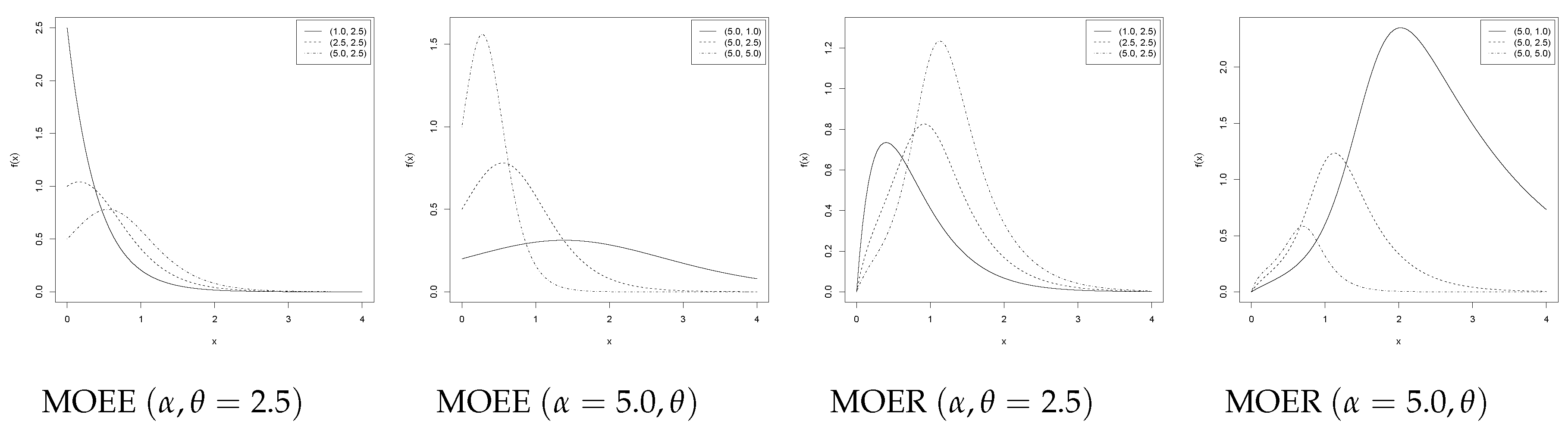
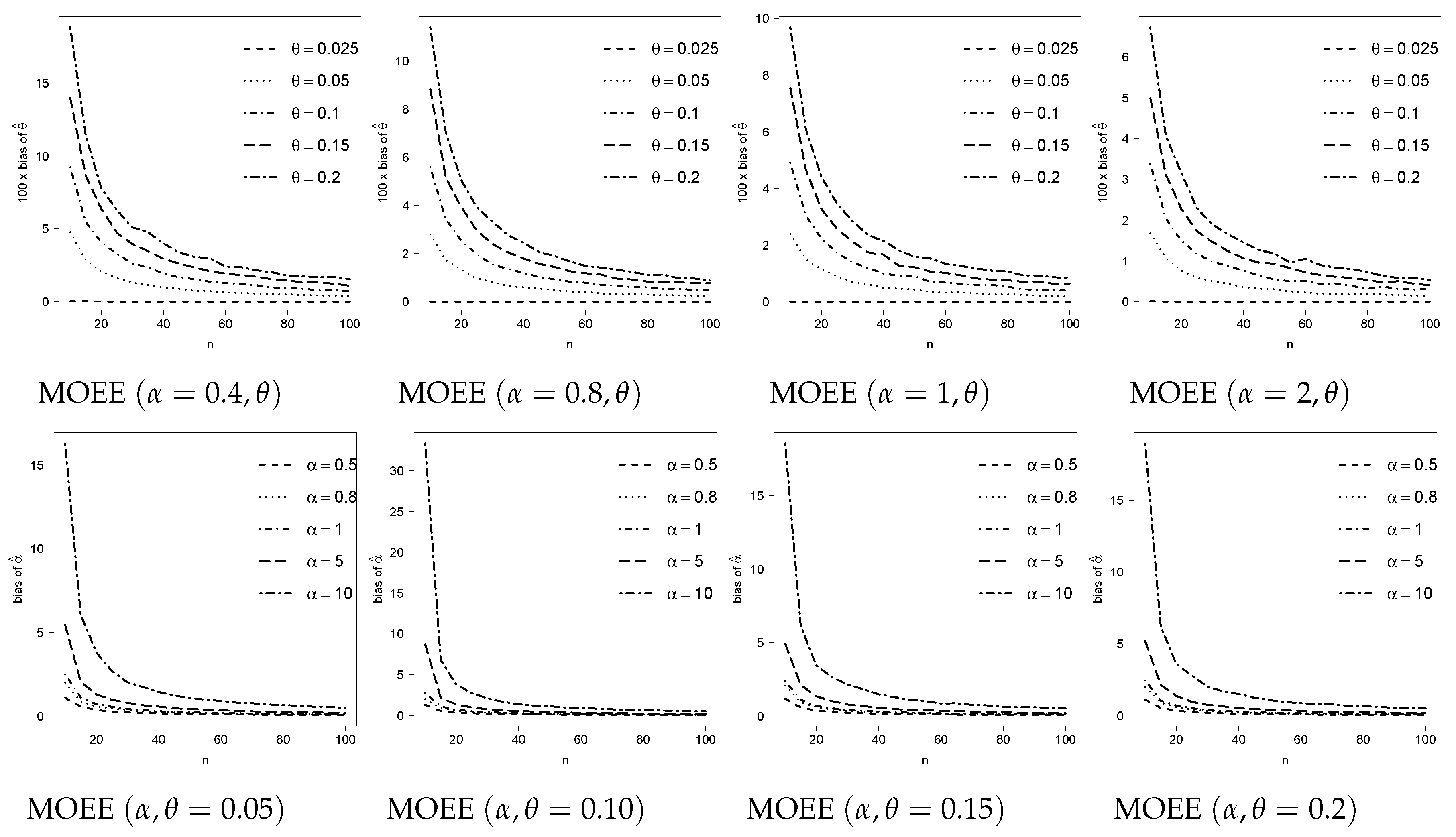
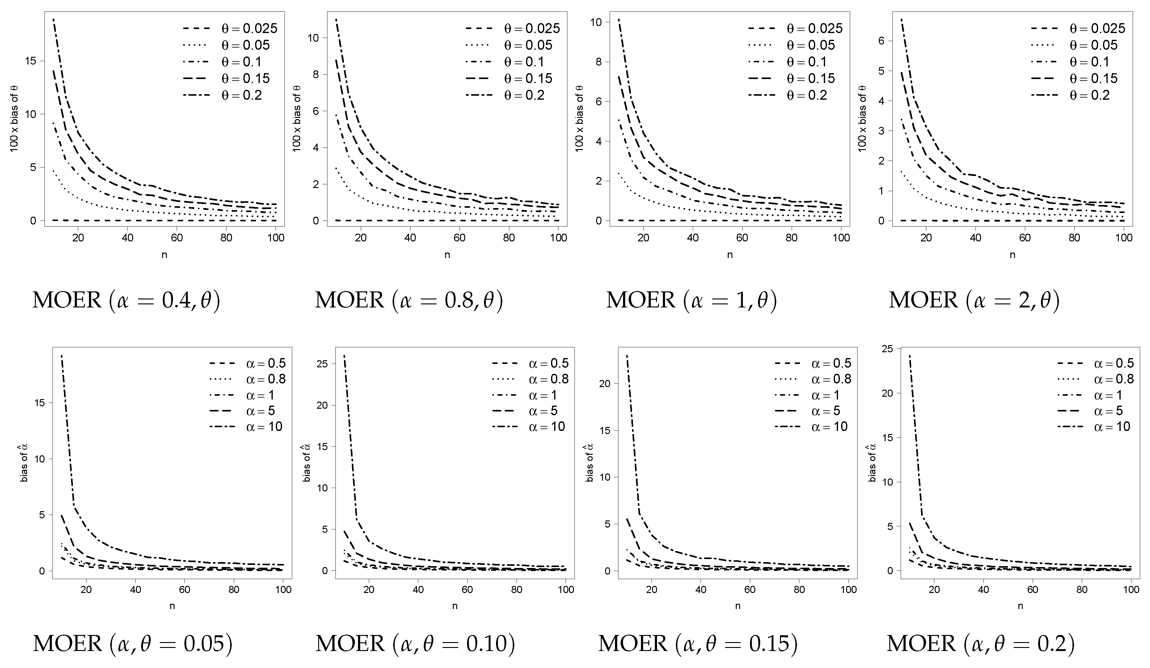
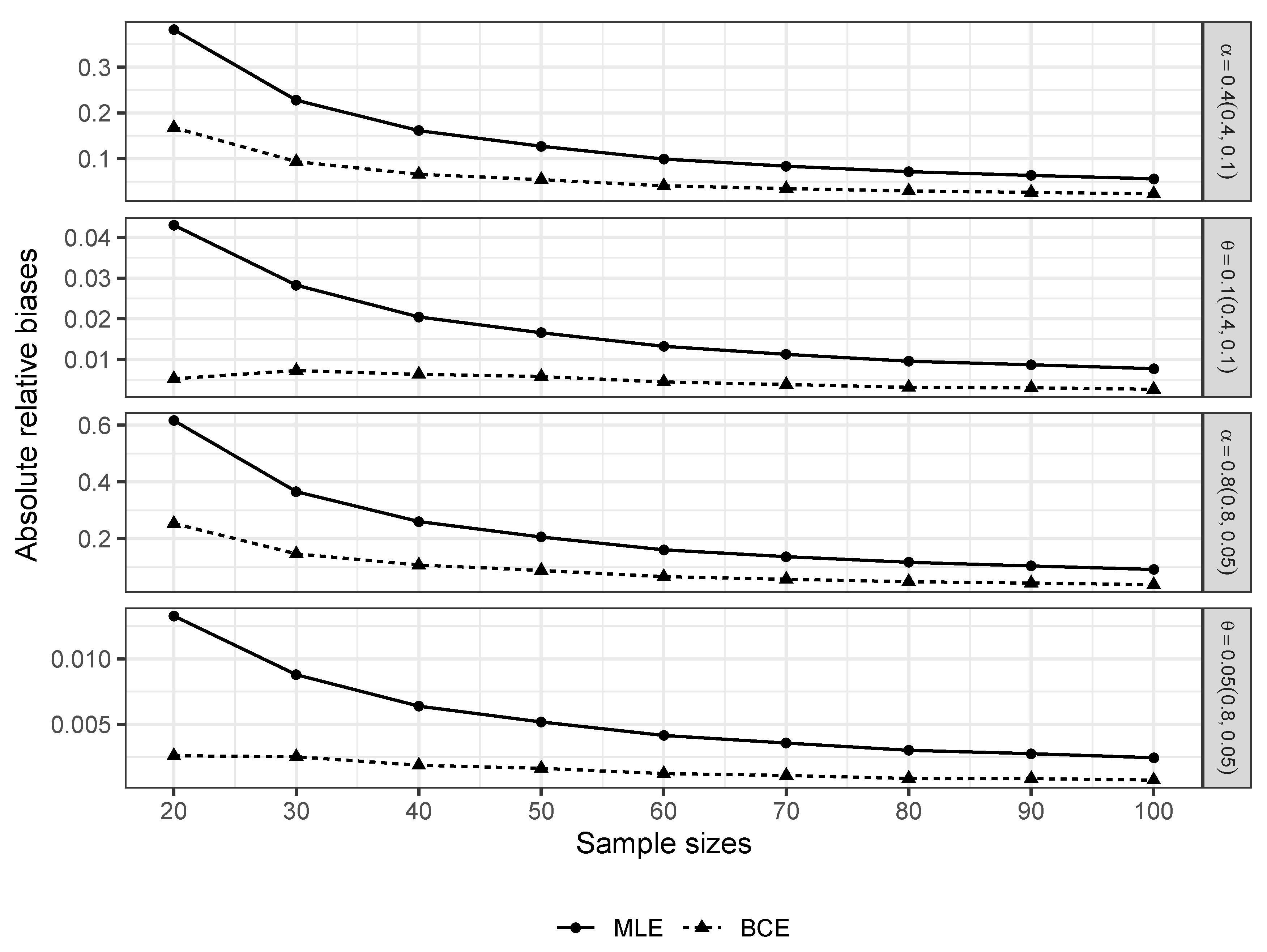
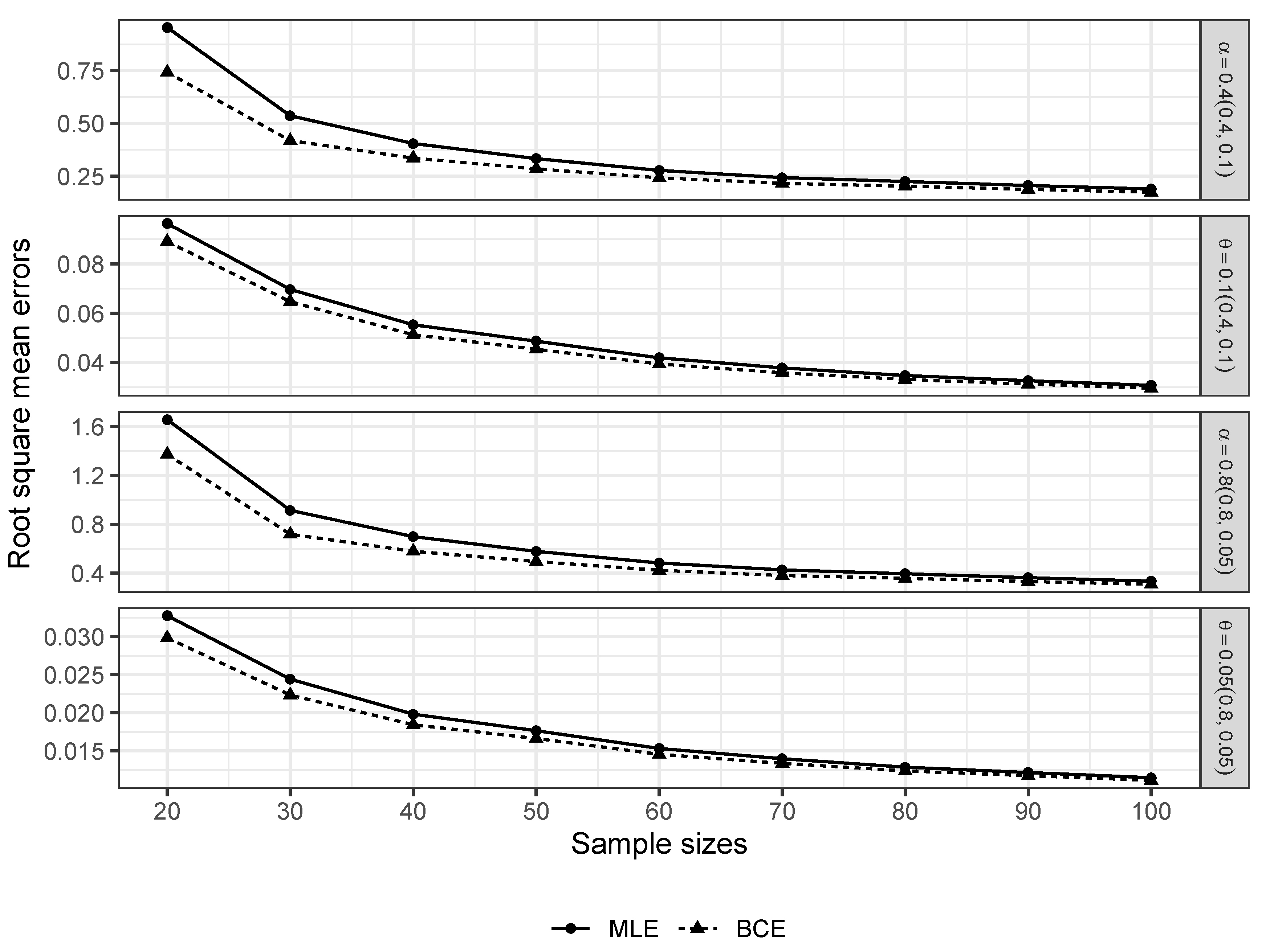
3.1. Reducing the Bias in the MOEE and MOER Models

We evaluate the performance of the MLE and BCE, described in Section 2, through a Monte Carlo simulation. The sample sizes considered are $n=10,20,\dots ,100$ and the total number of replications was set at 5000. All simulations were performed using the R software [32].

The MOEE model with true parameter vectors $(\alpha =1.5,\theta =1.5)$ and $(\alpha =2.5,\theta =1.5)$ and MOER model with true parameter vectors $(\alpha =0.4,\theta =0.1)$ and $(\alpha =0.8,\theta =0.05)$ were used as an illustration. However, with other sets of $(\alpha ,\theta )$, the conclusions obtained in this study were similar.

In each of the 5000 replications, for each scenario, the data were drawn from the respective model and we computed the MLE (say $\widehat{\alpha }$ and $\widehat{\theta }$) and the BCE (say ${\widehat{\alpha }}_M$ and ${\widehat{\theta }}_M$). Additionally, we computed the estimated absolute relative bias (ARB) and the estimated root mean square errors (RMSE) which are defined, respectively, as $\left|\mathbb{E}\left(\widehat{\alpha }\right)-\alpha \right|/\alpha$ and $\sqrt{\mathbb{E}\left[{(\widehat{\alpha }-\alpha )}^2\right]}$ for the MLE of $\alpha$ (for the BCE, we replace $\widehat{\alpha }$ by ${\widehat{\alpha }}_M$ and the terms are analogous for the estimators of $\theta$). In

Table 1. Absolute value of relative biases and the RMSE (in parentheses) in the MOEE distribution.

	$\mathit{\alpha }=1.5$, $\mathit{\theta }=1.5$				$\mathit{\alpha }=2.5$, $\mathit{\theta }=1.5$
n	Estimator of $\mathit{\alpha }$		Estimator of $\mathit{\theta }$		Estimator of $\mathit{\alpha }$		Estimator of $\mathit{\theta }$
	MLE	BCE	MLE	BCE	MLE	BCE	MLE	BCE
10	2.329	1.374	0.385	0.062	2.481	1.588	0.297	0.116
	(0.855)	(0.656)	(1.283)	(1.104)	(0.851)	(0.642)	(1.036)	(0.924)
20	0.711	0.311	0.184	0.033	0.715	0.385	0.144	0.011
	(0.780)	(0.693)	(0.743)	(0.670)	(0.780)	(0.664)	(0.619)	(0.578)
30	0.414	0.170	0.122	0.030	0.408	0.193	0.096	0.017
	(0.749)	(0.699)	(0.564)	(0.520)	(0.749)	(0.700)	(0.474)	(0.447)
40	0.295	0.120	0.089	0.021	0.290	0.130	0.070	0.014
	(0.732)	(0.692)	(0.465)	(0.435)	(0.736)	(0.700)	(0.394)	(0.376)
50	0.233	0.098	0.072	0.019	0.228	0.099	0.057	0.012
	(0.713)	(0.686)	(0.417)	(0.395)	(0.717)	(0.690)	(0.354)	(0.339)

, we present the results using MOEE for $n=10,\dots ,50$. Since the results were the same using MOER, we preferred to present them through Figure 4 and Figure 5 because it is more interesting for large sample sizes.

We can make some observations from Table 1 and Figure 4 and Figure 5. First, the ARB is not negligible for small samples, but the BCE ${\widehat{\alpha }}_M$ has a smaller ARB than $\widehat{\alpha }$. In small sample sizes especially (say $n=10,20,30$), the ARB is half the ARB for $\widehat{\alpha }$. In larger sample sizes, the ARB, hence the bias, of the MLE continues larger than the BCE, but as expected, the two terms become closer as n increases. We also note that the RMSE of ${\widehat{\alpha }}_M$ is smaller than the RMSE of $\widehat{\alpha }$. On the other hand, the original proposal only considered a bias reduction methodology for ${\widehat{\alpha }}_M$; this also produces an improvement in the behavior of ${\widehat{\theta }}_M$ in comparison with $\widehat{\theta }$, provided that the bias and RMSE for ${\widehat{\theta }}_M$ is less than the bias and RMSE for $\widehat{\theta }$, in both MOEE and MOER. This suggests that in models where g is indexed by a vector $\lambda$ with one or more parameters, the improvement in terms of bias and RMSE should benefit the BCE of $\alpha$ and $\lambda$ jointly, as we will illustrate in Section 4. The histograms of the estimates for ${\widehat{\alpha }}_M$ and ${\widehat{\theta }}_M$ show that their respective distributions are less asymmetrical than $\widehat{\alpha }$ and $\widehat{\theta }$; these histograms were omitted for the sake of brevity. As there is no theoretical explanation that justifies this behavior, we can interpret it as a side-effect of the BCE procedure.

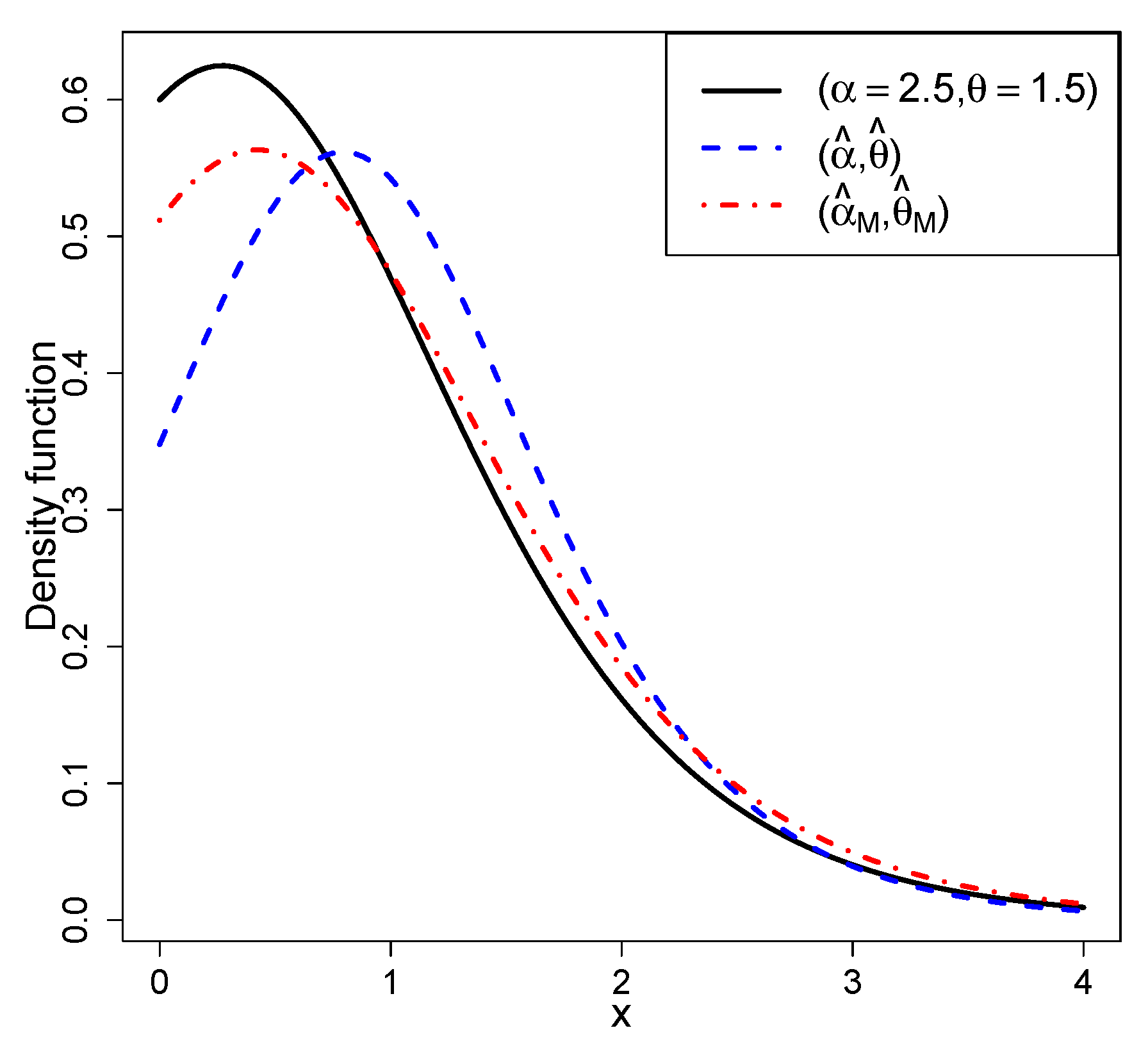
3.2. A Simulated Example with Outliers

In this simulation study, we show the impact of the bias in an estimation of the MOEE distribution in presence of an outlier. From the model with $\alpha =2.5$ and $\theta =1.5$, we sampled 10 observations: $x=(0.554,0.960,1.099,1.200,0.424,0.223,2.883,0.938,0.276,1.545)$. To illustrate the robustness of the method, we replaced the first observation $x_1$ by $x_1+1.5\times \mathrm{sd}\left(x\right)=1.732$. This perturbation scheme is usually used in local influence. In

Table 2. Estimates for the parameters in a simulated data set.

Parameter	True	Original		with Outlier
	Value	MLE	BCE	MLE	BCE
$\alpha$	2.5	3.873	2.174	5.223	2.866
$\theta$	1.5	1.839	1.464	1.817	1.467

, we present the estimate for the original data set and the data set with presence of the outlier. Please note that the impact on the estimators of $\alpha$ differs further for the MLE than for the BCE. Additionally, as expected, the bias for the MLE is considerably smaller than the bias for the BCE. On the other hand, the estimations of $\theta$ seem not to be much impacted by the presence of the outlier. Figure 6 shows the MOEE pdf of this artificial data set compared with the pdf estimated by MLE and BCE. We also note that the pdf estimated by BCE is closer to the pdf with the original parameters than the pdf estimated by MLE.

4. Two Applications

In this section, we present two real data applications illustrating the gains in bias reduction in the MOEE and MOER models.

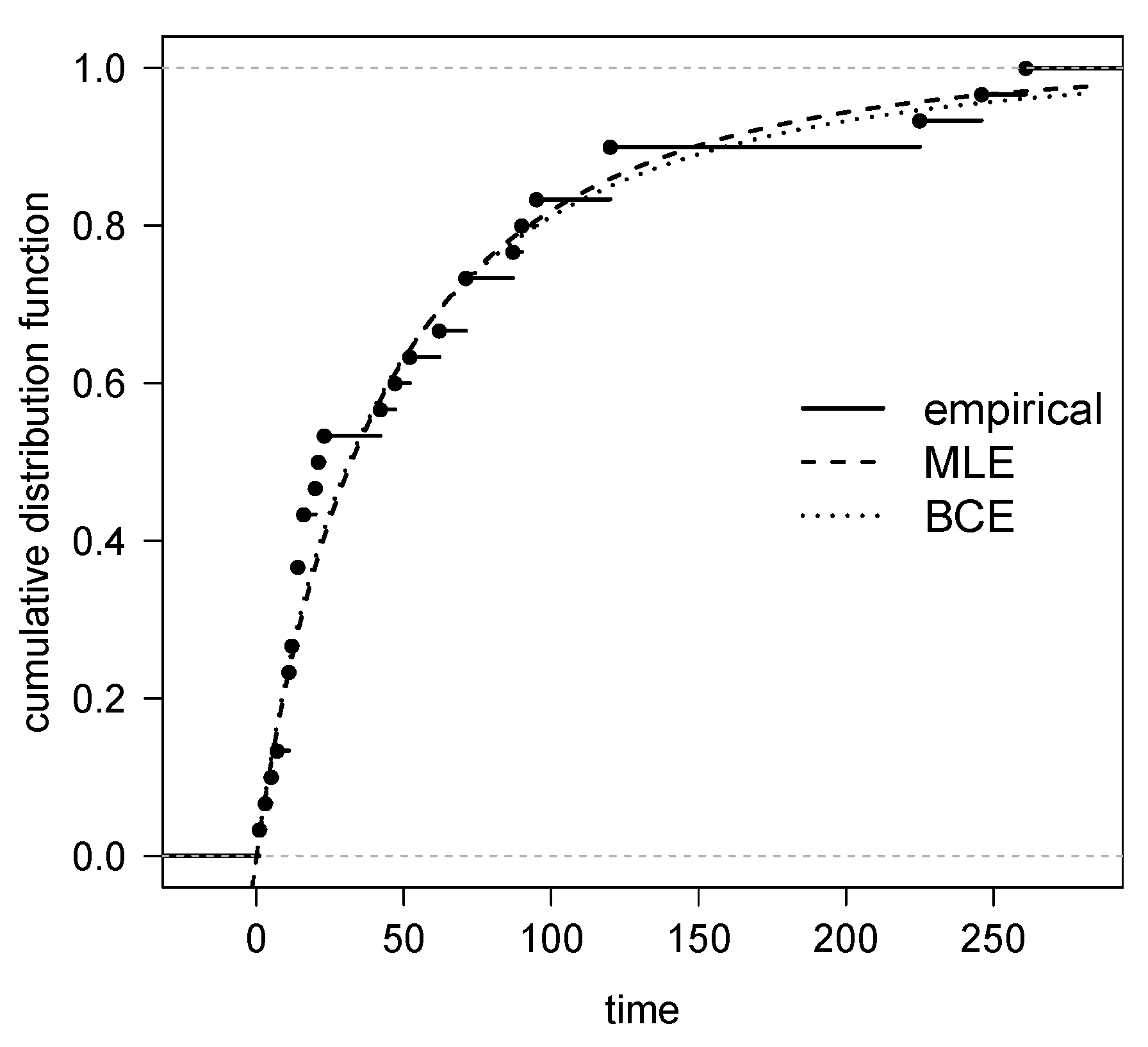
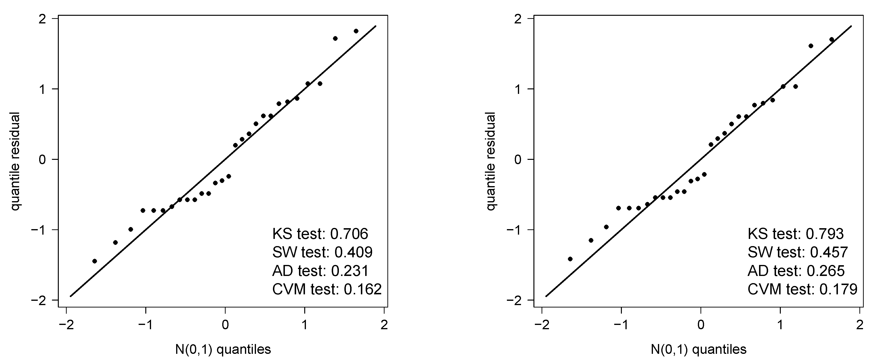
4.1. Air Conditioning System of an Airplane Data Set

In this section, we analyze the dataset presented by Linhart and Zucchini [33] (p. 69) to illustrate our method of estimation in MOEE. The data are failure times of the air conditioning system of an airplane: 23, 261, 87, 7, 120, 14, 62, 47, 225, 71, 246, 21, 42, 20, 5, 12, 120, 11, 3, 14, 71, 11, 14, 11, 16, 90, 1, 16, 52, 95. We use the MOEE distribution to fit this data.

Table 3. Estimates for MOEE distribution in the air conditioning system of an airplane. Standard errors are presented in parenthesis.

Parameter	MLE	BCE
$\alpha$	0.380 (0.272)	0.285 (0.225)
$\theta$	0.010 (0.005)	0.008 (0.005)

presents the parameter estimates using the MLE and the preventive method of estimation. In agreement with our simulation study, the MLE overestimated parameter vector $\lambda$, especially for parameter $\alpha$. In this case, besides the benefits related to bias reduction of BCE in comparison with MLE, we observe that the estimated standard error for $\alpha$ is lower with the BCE than with the MLE. Figure 7 shows the empirical cdf for this data set compared with the estimated cdf for MOEE in the MLE and BCE. We remark that the Kolmogorov-Statistic (i.e., the maximum distance between the empirical and estimated cdf) is reduced from 0.1284 to 0.1185 considering MLE versus BCE. Finally, Figure 8 presents the randomized quantile residuals [34] for MLE and BCE. If the model is correct, those models are a random sample from the standard normal distribution. Several normality test are presented in the figure. Please note that all p-values related to those tests are greater for the BCE than for the MLE, suggesting a better fit of the BCE estimates.

4.2. Precipitation Data Set

This data set is obtained from Hinkley [35]. It consists of thirty successive values of March precipitation (measured in inches) in Minneapolis/St Paul. We consider this illustration of our method of estimation in MOER.

Table 4. Estimates, standard errors (SE) and bias (estimated via bootstrap) for MOER distribution in precipitation data set.

Parameter	MLE			BCE
	Estimate	SE	Bias	Estimate	SE	Bias
$\alpha$	0.514	0.351	0.255	0.394	0.270	0.213
$\theta$	0.185	0.087	0.041	0.157	0.080	0.039

presents the parameter estimates using maximum likelihood estimation and the preventive method of estimation. MLE overestimated parameter vector $\lambda$ in comparison with BCE. Also, the bias (estimated via bootstrap) is reduced in both parameters, as well the standard errors. Figure 9 shows the histogram for this data set compared with the estimated pdf for MOER in MLE and BCE.

Table 5. Approximated 95% CI for the q-th quantile of the MOER model in precipitation data set based on MLE and BCE.

q	MLE		BCE
	95% IC	Width	95% IC	Width
0.10	(0.5313–0.5629)	0.0316	(0.5106–0.5361)	0.0256
0.25	(0.8845–0.9619)	0.0773	(0.8553–0.9210)	0.0657
0.50	(1.4225–1.5678)	0.1452	(1.3882–1.5261)	0.1379
0.75	(2.1286–2.3566)	0.2281	(2.1067–2.3593)	0.2526
0.90	(2.8078–3.2958)	0.4880	(2.8108–3.4102)	0.5994
0.99	(3.5118–5.7177)	2.2059	(3.3545–6.3541)	2.9996

shows the approximated 95% confidence interval (CI) for the q-th quantile (say, $x_q$) in this model based on MLE and BCE considering different values for q (see Appendix A for details of the construction of this approximated CI). Finally, Figure 10 shows the width of these CI’s based on the two methods. Please note that BCE provides a lower width for $q\le 0.592$ and MLE provides a lower width for $q>0.592$.

5. Concluding Remarks

We derived an expression for the bias of MLE related to the $\alpha$ parameter in the Marshall-Olkin extended family. The expression found allowed us to construct a procedure, using penalized likelihood, which generates a modified MLE with reduced bias. This is a useful development. In many cases, it is very difficult or even impossible to find bias-corrected maximum likelihood estimators for specific distribution families; we were able to find them for the Marshall-Olkin extended family. The reduced-bias estimator presents better performance than the corresponding procedures based on the initial estimator; for sample sizes equal to 10 or 20, the bias reduction was approximately 50%. The mean square error was also reduced. The scheme to use BCE is quite simple to implement in statistical softwares such as R. As mentioned by Firth [28]: “the merits of bias reduction in any particular problem will depend on several factors, including the skewness of the maximum likelihood estimator.” Since the MLE of the parameters in the Marshall-Olkin extended family is quite biased, this is an indication that its distribution is asymmetrical. For a future work, we suggest the study of the skewness of the MLE in the $MO{E}_g$, as, recently performed by Magalhães et al. [36] for the varying beta regression model (BRM) and Magalhães et al. [37] for Weibull censored data (WCD). In the first work, the authors showed that the MLE of the precision parameter is quite asymmetrical, while in the second, the MLE of the parameters is close to symmetry. This agrees with bias literature for the respective models, which showed that estimates of the precision parameters in the varying beta regression model are highly biased while the estimates in WCD are little biased. Since there is no closed-form for the skewness coefficient of the MLE of the $MO{E}_g$, it will be a greater contribution to this family of distributions.

References

1. Marshall, A.W.; Olkin, I. A new method for adding a parameter to a family of distributions with application to the exponential and weibull families. Biometrika 1997, 84, 641–652. [Google Scholar] [CrossRef]
2. Marshall, A.W.; Olkin, I. Life Distributions. Structure of Nonparametric, Semipara- Metric and Parametric Families; Springer: New York, NY, USA, 2007. [Google Scholar]
3. Castellares, F.; Lemonte, A.J. On the Marshall-Olkin extended distributions. Commun. Stat. Theory Methods 2016, 45, 4537–4555. [Google Scholar] [CrossRef]
4. Ghitany, M.E. Marshall-Olkin extended pareto distribution and its application. Int. J. Appl. Math. 2005, 18, 17–32. [Google Scholar]
5. Ghitany, M.E.; Al-Hussaini, E.K.; Jarallah, R.A. Marshall-Olkin extended Weibull distribution and its application to censored data. J. Appl. Stat. 2005, 32, 1025–1034. [Google Scholar] [CrossRef]
6. Ristic, M.M.; Kanichukattu, J.; Joseph, A. A marshall-olkin gamma distribution and minification process. STARS Int. J. Sci. 2007, 1, 107–117. [Google Scholar]
7. Ghitany, M.E.; Al-Awadhi, F.A.; Alkhalfan, L.A. Marshall-olkin extended lomax distribution and its application to censored data. Commun. Stat. Theory Methods 2007, 36, 1855–1866. [Google Scholar] [CrossRef]
8. Ghitany, M.E.; Kotz, S. Reliability properties of extended linear failure-rate distributions. Probab. Eng. Inf. Sci. 2007, 21, 441–450. [Google Scholar] [CrossRef]
9. Jayakumar, K.; Mathew, T. On a generalization to Marshall–Olkin scheme and its application to Burr type XII distribution. Stat. Pap. 2008, 49, 421–439. [Google Scholar] [CrossRef]
10. García, V.; Gómez, E.; Vásquez-Polo, F. A new skew generalization of the normal distribution: Properties and applications. Comput. Stat. Data Anal. 2010, 54, 2021–2034. [Google Scholar] [CrossRef]
11. Gómez-Déniz, E. Another generalization of the geometric distribution. Test 2010, 19, 399–415. [Google Scholar] [CrossRef]
12. Lemonte, A. A new extension of the Birnbaum-Saunders distribution. Braz. J. Probab. Stat. 2013, 27, 133–149. [Google Scholar] [CrossRef]
13. Cordeiro, G.; Lemonte, A. On the Marshall-Olkin extended Weibull distribution. Stat. Pap. 2013, 54, 333–353. [Google Scholar] [CrossRef]
14. Cordeiro, G.; Lemonte, A.; Ortega, E. The Marshall-Olkin family of distributions: Mathematical properties and new models. J. Stat. Theory Pract. 2013, 8, 343–366. [Google Scholar] [CrossRef]
15. Alshangiti, A.M.; Kayid, M.; Alarfaj, B. A new family of Marshall-Olkin extended distributions. J. Comput. Appl. Math. 2014, 271, 369–379. [Google Scholar] [CrossRef]
16. Alizadeh, M.; Cordeiro, G.M.; De Brito, E.; Demétrio, C.G.B. The beta Marshall-Olkin family of distributions. J. Stat. Distrib. Appl. 2015, 2, 1–18. [Google Scholar] [CrossRef] [Green Version]
17. Ristić, M.; Kundu, D. Marshall-Olkin generalized exponential distribution. Metron 2015, 73, 317–333. [Google Scholar] [CrossRef]
18. Benkhelifa, L. The Marshall-Olkin extended generalized Lindley distribution: Properties and applications. Commun. Stat. Simul. Computation. 2017, 46, 8306–8330. [Google Scholar] [CrossRef]
19. Afify, A.Z.; Cordeiro, G.M.; Yousof, H.M.; Saboor, A.; Ortega, E.M.M. The Marshall-Olkin additive Weibull distribution with variable shapes for the hazard rate. Hacet. J. Math. Stat. 2018, 47, 365–381. [Google Scholar] [CrossRef]
20. Javed, M.; Nawaz, T.; Irfan, M. The Marshall-Olkin Kappa distribution: Properties and applications. J. King Saud Univ. Sci. 2019, 31, 684–691. [Google Scholar] [CrossRef]
21. Mansoor, M.; Tahir, M.H.; Cordeiro, G.M.; Provost, S.B.; Alzaatreh, A. The Marshall-Olkin logistic-exponential distribution. Commun. Stat. Theory Methods 2019, 48, 220–234. [Google Scholar] [CrossRef]
22. Yousof, H.M.; Afify, A.Z.; Alizadeh, M.; Nadarajah, S.; Aryal, G.; Hamedani, G. The Marshall-Olkin generalized-G family of distributions with applications. Statistica 2018, 78, 273–295. [Google Scholar]
23. Durrans, S.R. Distributions of fractional order statistics in hydrology. Water Resour. Res. 1992, 28, 1649–1655. [Google Scholar] [CrossRef]
24. Guney, Y.; Tuac, Y.; Arslan, O. Marshall-Olkin distribution: Parameter estimation and application to cancer data. J. Appl. Stat. 2017, 44, 2238–2250. [Google Scholar] [CrossRef]
25. Korkmaz, M.Ç.; Cordeiro, G.M.; Yousof, H.M.; Pescim, R.R.; Afify, A.Z.; Nadarajah, S. The Weibull Marshall-Olkin family: Regression model and application to censored data. Commun. Stat. Theory Methods 2019, 48, 4171–4194. [Google Scholar] [CrossRef]
26. Nassar, M.; Kumar, D.; Dey, S.; Cordeiro, G.M.; Afify, A.Z. The Marshall-Olkin alpha power family of distributions with applications. J. Comput. Appl. Math. 2019, 1, 41–53. [Google Scholar] [CrossRef]
27. Cox, D.R.; Snell, E.J. A general definition of residuals. J. R. Society. Ser. B Methodol. 1968, 30, 248–275. [Google Scholar] [CrossRef]
28. Firth, D. Bias reduction of maximum likelihood estimates. Biometrika 1993, 80, 27–38. [Google Scholar] [CrossRef]
29. Sartori, N. Bias prevention of maximum likelihood estimates for scalar skew normal and skew t distributions. J. Stat. Plan. Inference 2006, 136, 4259–4275. [Google Scholar] [CrossRef]
30. Cordeiro, G.M.; Cribari-Neto, F. An introduction to Bartlett Corrections and Bias Reduction; Springer: Berlin/Heidelberg, Geramny, 2014. [Google Scholar]
31. Arrué, J.; Arellano-Valle, R.B.; Gómez, H.W. Bias reduction of maximum likelihood estimates for a modified skew normal distribution. J. Stat. Comput. Simul. 2016, 86, 2967–2984. [Google Scholar] [CrossRef]
32. R Core Team. R: A Language and Environment for Statistical Computing; R Foundation for Statistical Computing: Vienna, Austria, 2017. [Google Scholar]
33. Linhart, H.; Zucchini, W. Model Selection; John Wiley and Sons: New York, NY, USA, 1986. [Google Scholar]
34. Dunn, P.; Smyth, G. Randomized quantile residuals. J. Comput. Graph. Stat. 1996, 5, 236–244. [Google Scholar]
35. Hinkley, D. On quick choice of power transformation. Am. Stat. 1977, 26, 67–69. [Google Scholar] [CrossRef]
36. Magalhães, T.M.; Botter, D.A.; Sandoval, M.C.; Pereira, G.H.A.; Cordeiro, G.M. Skewness of maximum likelihood estimators in the varying dispersion beta regression model. Commun. Stat. Theory Methods 2019, 48, 4250–4260. [Google Scholar] [CrossRef]
37. Magalhães, T.M.; Gallardo, D.I.; Gómez, H.W. Skewness of maximum likelihood estimators in the weibull censored data. Symmetry 2019, 11, 1351. [Google Scholar] [CrossRef] [Green Version]
Figure 1. Pdf for MOEE and MOER models under different combinations of parameters.
Symmetry 12 00851 g001
Figure 2. Estimated bias for the MLE of α and θ in the MOEE( α , θ ) under different scenarios based on 5000 replicates.
Symmetry 12 00851 g002
Figure 3. Estimated bias for the MLE of α and θ in the MOER( α , θ ) under different scenarios based on 5000 replicates.
Symmetry 12 00851 g003
Figure 4. Estimated bias for the MLE and BCE of α and θ in the MOER distribution.
Symmetry 12 00851 g004
Figure 5. Estimated RMSE for the MLE and BCE of α and θ in the MOER distribution.
Symmetry 12 00851 g005
Figure 6. Estimated RMSE for the MLE and BCE of α and θ in the MOEE.
Symmetry 12 00851 g006
Figure 7. Empirical cdf and cdf estimated by MLE and BCE in the air conditioning system of an airplane data set considering the MOEE model.
Symmetry 12 00851 g007
Figure 8. Randomized quantile residuals for MOEE in the air conditioning system of an airplane. Left panel: MLE. Right panel: BCE. The p-values for the following normality tests are also presented: Kolmogorov-Smirnov (KS), Shapiro-Wilks (SW), Anderson-Darling (AD) and Cramer-von Mises (CVM)
Symmetry 12 00851 g008
Figure 9. Histogram and estimated pdf for MLE and BCE considering the MOER distribution in the precipitation data set.
Symmetry 12 00851 g009
Figure 10. Width of 95% CI for quantiles of MOER model considering the MLE (continuous line) and BCE (dashed line).
Symmetry 12 00851 g010