Pythagorean Fuzzy Matroids with Application

Abstract

The Pythagorean fuzzy models deal with graphical and algebraic structures in case of vague information related to membership and non-membership grades. Here, we use Pythagorean fuzzy sets to generalize the concept of vector spaces and discuss their basis and dimensions. We also highlight the concept of Pythagorean fuzzy matroids and examine some of their fundamental characteristics like circuits, basis, dimensions, and rank functions. Additionally, we explore the concept of Pythagorean fuzzy matroids in linear algebra, graph theory, and combinatorics. Finally, we demonstrate the use of Pythagorean fuzzy matroids for minimizing the time taken by a salesman in delivering given products.

1. Introduction

The fields of graph theory, combinatorics, and fuzzy set theory are reckoned to be closely linked. In the last few decades, these fields have achieved renewed attention from the research community, where matroids and matroids theory has been the main focus of much dynamic research. This concept of matroids was first presented by Whitney [1], where he developed a significant relationship for the fundamental parameters of graph theory, combinatorics, and several other aspects of mathematics. After the introduction of a new term, namely fuzzy logic by Zadeh [2] in 1965, the theory of fuzzy sets became popular among many researchers. Atanassov [3] generalized fuzzy sets and offered the concept of “intuitionistic fuzzy sets (IFSs)” by explaining the degree of membership and non-memberships whose sum was not greater than 1. Later on, this idea of intuitionistic fuzzy sets was studied extensively for the wide scope of applications in numerous fields [4,5,6,7,8]. A new type of fuzzy sets, known as Pythagorean fuzzy sets (PFSs), proposed by Yager [9,10], are regarded as more general than IFSs and are characterized into a membership and non-membership degree, with the square sum not greater than 1.

The idea of “fuzzy vector spaces” was first presented by Katsaras and Liu [11]. It was further developed by Lowen [12] who generalized normal linearly independence of vector space for fuzzy vector space and discussed its finite dimensions. Lubczonok [13] contributed to this field by defining dimensions of fuzzy vector spaces as infinity and explaining their properties. Later, many studies investigated several properties of vector spaces based on several fuzzy set types [14,15,16,17].

A graph is of great significance in developing a better understanding of information and exhibiting the relationship between objects. The fuzzification of graphs is a significant area of research with increasing connections to the fields of pure and applied mathematics. Kauffman (1973) was the first to put forward the concept of fuzzy graphs [18]. Later, some of the theoretical concepts regarding paths and cycles in these graphs were characterized by Rosenfeld [19]. Presently, several advanced modifications of graph theory have been simplified to model the uncertainties in reliability theory as well as graphical networking problems. Moreover, the study of fuzzy graphs based on different sets, such as intuitionistic fuzzy graphs, intuitionistic fuzzy hypergraphs, m-polar fuzzy graphs, edge-regular q-rung picture fuzzy graphs, Pythagorean fuzzy graphs (PFGs), and n Pythagorean fuzzy graphs have been carried out by different researchers [20,21,22,23,24,25,26]. Recently, some new operations like rejection, symmetric difference, residue product, and maximal product have also been proposed for PFGs (see [27]). Goetschel and Voxman [28], proposed a new idea of fuzzy matroids and defined their rank functions. They also discussed basis, circuits, and other concepts related to the fuzzy matroids in their subsequent work [29,30]. With the passage of time, different kind of fuzzy matroids were presented, based on varied definitions of fuzzy sets and their axioms [31,32,33,34,35,36,37]. Sarwar and Akram [38], highlighted the idea of m-polar fuzzy matroids and also discussed their pivotal properties. However, all fuzzy matroids are interpreted by the direct generalization of the axiomatic definition of crisp to fuzzy matroids. For details about the notions used in this paper, the readers are referred to [27,28,29,39].

In this study, firstly, we define Pythagorean fuzzy vector spaces, their basis, and dimensions. Then matroids are defined based on PFSs and are named as Pythagorean fuzzy matroids. Here, Pythagorean fuzzy matroids are applied to linear algebra as well as graph theory, and combinatorics with some of their basic properties. The notions of circuits, basis, dimensions, closure of Pythagorean fuzzy matroids, and more importantly Pythagorean fuzzy rank function are also discussed here in detail. Moreover, we supported our proposed idea by explaining the graphical view of a salesman regarding his package delivery, using Pythagorean fuzzy matroids.

2. Preliminaries

This section presents basic notions related to PFSs, crisp matroids, and fuzzy matroids which are useful for further advancement.

Definition 1

([1]). Let $X\ne \varphi$ be a finite universe with power set $P(X)$. For $\mathcal{A}\subseteq P(X)$, the pair $\mathcal{M}=(X,\mathcal{A})$ is said to be a matroid if it satisfies the following conditions,

1.

$\varphi \in \mathcal{A}$;

2.

If $A_1\subset A_2$ and $A_2\in \mathcal{A}$, then $A_1\in \mathcal{A}$;

3.

If $A_1,A_2\in \mathcal{A}$ with $\mid A_2\mid <\mid A_1\mid$, then there exists $A_3\in \mathcal{A}$ such that $A_2\subset A_3\subseteq A_1\cup A_2$, where $\mid A\mid$ is a cardinality of the set A.

Here $\mathcal{A}$ is called the collection of independent sets in $\mathcal{M}$.

The set $A\in \mathcal{A}$ is called maximal independent if there does not exist $A^{\prime }$ in $\mathcal{A}$ such that $A\subset A^{\prime }$.

Definition 2

([1]). Let $\mathcal{M}=(X,\mathcal{A})$ be a matroid and $B\in \mathcal{A}$. Then B is a base of $\mathcal{M}$ if B is maximal in $\mathcal{A}$ and $\mathcal{B}(\mathcal{M})$ is the set family of all bases.

Definition 3

([1]). A subset $C\subseteq X$ is called dependent if C is not in $\mathcal{A}$. A minimal dependent set (inclusion wise minimal in $P(X)\backslash \mathcal{A}$) is called circuit of $\mathcal{M}$ and $\mathcal{C}(\mathcal{M})$ is the collection of all circuits of $\mathcal{M}$.

Definition 4

([2,40]). A fuzzy set υ in a universe X is defined as a membership function $\upsilon :X\to [0,1]$ i.e.,

$$\upsilon =\{\langle x,\upsilon (x)\rangle \mid x\in X\}.$$

Here, $F(X)$ denotes the family of all fuzzy sets. The support and cardinality of a fuzzy set $\upsilon \in F(X)$ defined as,

(i).

$supp(\upsilon )=\{x\in X\mid \upsilon (x)>0\}$;

(ii).

$\mid \upsilon \mid ={\sum }_{x\in X}(\upsilon (x))$.

Definition 5

([28]). Let $F(X)$ be the family of all fuzzy sets on a finite universe $X\ne \varphi$ and $\mathcal{A}\subseteq F(X)$. The pair $\mathcal{FM}=(X,\mathcal{A})$ is called fuzzy matroid if it satisfies for any fuzzy sets ${\upsilon }_1,{\upsilon }_2,{\upsilon }_3$,

1.

$\varphi \in \mathcal{A}$;

2.

If ${\upsilon }_1\subset {\upsilon }_2 and {\upsilon }_2\in \mathcal{A}, then {\upsilon }_1\in \mathcal{A}, where {\upsilon }_1\subset {\upsilon }_2 means {\upsilon }_1(x)<{\upsilon }_2(x)$, for all $x\in X$;

3.

If ${\upsilon }_1,{\upsilon }_2\in \mathcal{A}$ with $\mid supp({\upsilon }_1)\mid <\mid supp({\upsilon }_2)\mid$, then there exists ${\upsilon }_3\in \mathcal{A}$ such that,

a. ${\upsilon }_1\subset {\upsilon }_3\subseteq {\upsilon }_1\cup {\upsilon }_2$, where $({\upsilon }_1\cup {\upsilon }_2)(x)=max\{{\upsilon }_1(x),{\upsilon }_2(x)\}, for any x\in X$.

b. $m({\upsilon }_3)\ge min\{m({\upsilon }_1),m({\upsilon }_2)\}$ where $m({\upsilon }_i)=min\{{\upsilon }_i(x):x\in supp({\upsilon }_i)\}$, for any $x\in X$ and i=1,2.

Here $\mathcal{A}$ is called the collection of independent fuzzy sets of $\mathcal{FM}$.

Definition 6

([9,10]). Let X be a finite universal set. Then the set of pairs $\xi =({\xi }^P,{\xi }^N)$ is called Pythagorean fuzzy set or PFS and is defined by,

$$\xi =\{\langle x,{\xi }^P(x),{\xi }^N(x)\rangle \mid x\in X\}.$$

The degree of membership and non-membership of $x\in X to \xi$ are given by the mappings ${\xi }^P:X\to [0,1]$ and ${\xi }^N:X\to [0,1]$ respectively, satisfying $0\le {({\xi }^P(x))}^2+{({\xi }^N(x))}^2\le 1$. For each $x\in X$, the hesitation degree ${\Im }_{\mathcal{P}}(x)$, which is given as,

$${\Im }_{\mathcal{P}}(x)=\sqrt{1-{({\xi }^P(x))}^2-{({\xi }^N(x))}^2}.$$

We write $\mathcal{P}(X)$ for the family of all PFSs on X. For $\xi \in \mathcal{P}(X)$, mentioned above, one has the following notations,

• $supp(\xi )=\{x\mid x\in X,{\xi }^P(x)>0,{\xi }^N(x)>0\}.$ Let $\xi (x)=({\xi }^P(x),{\xi }^N(x))$, for any $x\in X$, then
  $\xi (x_1){<}^{*}\xi (x_2) \mathrm{if} \mathrm{and} \mathrm{only} \mathrm{if} {\xi }^P(x_1)<{\xi }^P(x_2) \mathrm{and} {\xi }^N(x_1)>{\xi }^N(x_2)$, for all $x_1, x_2\in X$;
• $m(\xi )=min\{\xi (x)\mid x\in supp(\xi )\},$ for the order relation ${<}^{*}$;
• $\mid \xi \mid ={\sum }_{x\in X}({\xi }^P(x),{\xi }^N(x))=({\sum }_{x\in X}{\xi }^P(x),{\sum }_{x\in X}{\xi }^N(x)).$

Definition 7

([9,10]). Let ${\xi }_1=\{\langle x,{\xi }_1^P(x),{\xi }_1^N(x)\rangle \mid x\in X\}$ and ${\xi }_2=\{\langle x,{\xi }_2^P(x),{\xi }_2^N(x)\rangle \mid x\in X\}$ be the two PFSs on X. The set operations defined on PFSs are as follows,

1.

${\xi }_1\subseteq {\xi }_2 if and only if {\xi }_1^P(x)\le {\xi }_2^P(x) and {\xi }_1^N(x)\ge {\xi }_2^N(x),\forall x\in X$;

2.

${\xi }_1\cup {\xi }_2=\{\langle x,max({\xi }_1^P(x),{\xi }_2^P(x)),min({\xi }_1^N(x),{\xi }_2^N(x))\rangle \mid x\in X\}$;

3.

${\xi }_1\cap {\xi }_2=\{\langle x,min({\xi }_1^P(x),{\xi }_2^P(x)),max({\xi }_1^N(x),{\xi }_2^N(x))\rangle \mid x\in X\}.$

To be more precise, call $\tilde{z}=({\xi }^P,{\xi }^N)$ Pythagorean fuzzy number (PFN) such that $0\le {({\xi }^P)}^2+{({\xi }^N)}^2\le 1$ with ${\xi }^P,{\xi }^N\in [0,1]$. Note that 0=(0,1) is the smallest Pythagorean fuzzy element and 1=(1,0) is the largest Pythagorean fuzzy element.

Definition 8

([39]). Let $\tilde{z}=({\xi }^P,{\xi }^N)$ be a PFN. A score function $\mathcal{S}$ of $\tilde{z}$ is defined as,

$$\mathcal{S}(\tilde{z})=\frac{1}{2}(1+{({\xi }^P)}^2-{({\xi }^N)}^2),\hspace{1em}0\le \mathcal{S}(\tilde{z})\le 1.$$

Definition 9

([39]). Let $\tilde{z}=({\xi }^P,{\xi }^N)$ be a PFN. An accuracy function $\mathcal{H}$ of $\tilde{z}$ is defined as,

$$\mathcal{H}(\tilde{z})={({\xi }^P)}^2+{({\xi }^N)}^2,\hspace{1em}0\le \mathcal{H}(\tilde{z})\le 1.$$

Definition 10

([39]). Let $\widetilde{z_1}=({\xi }_1^P,{\xi }_1^N)$ and $\widetilde{z_2}=({\xi }_2^P,{\xi }_2^N)$ be two PFNs. The comparing relation between two PFNs is defined as follows,

(i).

If $\mathcal{S}(\widetilde{z_1})<\mathcal{S}(\widetilde{z_2})$, then $\widetilde{z_1}<\widetilde{z_2}$;

(ii).

If $\mathcal{S}(\widetilde{z_1})=\mathcal{S}(\widetilde{z_2})$, then

(a). If $\mathcal{H}(\widetilde{z_1})<\mathcal{H}(\widetilde{z_2})$, then $\widetilde{z_1}<\widetilde{z_2}$,

(b). If $\mathcal{H}(\widetilde{z_1})=\mathcal{H}(\widetilde{z_2})$, then $\widetilde{z_1}=\widetilde{z_2}$.

Definition 11

([27]). Let $G=(V,E)$ be a graph. Consider $V^{\prime }$ and $E^{\prime }$ are two PFSs in V and $E\subseteq V\times V$ respectively. The pair $G^{\prime }=(V^{\prime },E^{\prime })$ is called Pythagorean fuzzy graph(PFG) and defined as,

$${\xi }_{E^{\prime }}^P(xy)\le min({\xi }_{V^{\prime }}^P(x),{\xi }_{V^{\prime }}^P(y)), {\xi }_{E^{\prime }}^N(xy)\ge max({\xi }_{V^{\prime }}^N(x),{\xi }_{V^{\prime }}^N(y)) where xy is an edge between x and y.$$

For each $x,y\in V,$ the mappings ${\xi }_{E^{\prime }}^P:V\times V\to [0,1] and {\xi }_{E^{\prime }}^N:V\times V\to [0,1]$ satisfies $0\le {({\xi }_{E^{\prime }}^P(xy))}^2+{({\xi }_{E^{\prime }}^N(xy))}^2\le 1$.

3. Pythagorean Fuzzy Matroids

This section presents Pythagorean fuzzy vector spaces with basic notions such as basis and dimensions. Here, we also define Pythagorean fuzzy matroids with their significant properties.

Definition 12.

Let $X\ne \varphi$ be a vector space over a field $\mathbb{F}$. The PFS $\xi =({\xi }^P,{\xi }^N)$ in X is called Pythagorean fuzzy vector space (PFVS) over X, if for $a,b\in \mathbb{F} and x,y\in X$ we have,

$${\xi }^P(ax+by)\ge min\left\{{\xi }^P(x),{\xi }^P(y)\right\},$$

and

$${\xi }^N(ax+by)\le max\left\{{\xi }^N(x),{\xi }^N(y)\right\}.$$

where mappings ${\xi }^P:X\to [0,1]$ and ${\xi }^N:X\to [0,1]$ satisfies $0\le {({\xi }^P(x))}^2+{({\xi }^N(x))}^2\le 1$. Then the pair $\tilde{X}=(X,\xi )$ called the set of all PFVSs over X.

Definition 13.

Let $\tilde{X}=\left(X,\xi \right)$ be a PFVS over $\mathbb{F}$. The set of vectors ${\left\{x_k\right\}}_{k=1}^n$ is called a Pythagorean fuzzy linearly independent in $\tilde{X}$ if,

1.

${\{x_k\}}_{k=1}^n$ is linearly independent;

2.

For any ${\{a_k\}}_{k=1}^n\subset \mathbb{F}$ we have,

$${\xi }^P\left(\sum _{k=1}^n{a}_k{x}_k\right)=\underset{k=1}{\overset{n}{min}}{\xi }^P(a_k{x}_k),$$

and

$${\xi }^N\left(\sum _{k=1}^n{a}_k{x}_k\right)=\underset{k=1}{\overset{n}{max}}{\xi }^N(a_k{x}_k).$$

Definition 14.

A set of vectors $\mathcal{B}={\{{\beta }_k\}}_{k=1}^n$ is called Pythagorean fuzzy basis in $\tilde{X}$, if the following conditions satisfies,

1.

$\mathcal{B}$ is basis in X;

2.

For any ${\{a_k\}}_{k=1}^n\subset \mathbb{F}$ we have,

$${\xi }^P\left(\sum _{k=1}^n{a}_k{\beta }_k\right)=\underset{k=1}{\overset{n}{min}}{\xi }^P(a_k{\beta }_k),$$

and

$${\xi }^N\left(\sum _{k=1}^n{a}_k{\beta }_k\right)=\underset{k=1}{\overset{n}{max}}{\xi }^N(a_k{\beta }_k).$$

Definition 15.

Let $\tilde{X}=(X,\xi )$ be a PFVS with basis $\mathcal{B}.$ Then the dimension of $\tilde{X}$ is defined as,

$$di{m}_P(\tilde{X})=\underset{\mathcal{B} is a basis of X}{sup}\left(\sum _{\beta \in \mathcal{B}}\left({\xi }^P(\beta ),{\xi }^N(\beta )\right)\right).$$

Example 1.

Let $X={\mathbb{R}}^2$ be a vector space over the field $\mathbb{R}$ and let $\xi =({\xi }^P,{\xi }^N)$ be a PFS in X. For each $\omega =(x,y)\in {\mathbb{R}}^2$, mappings ${\xi }^P:X\to [0,1]$ and ${\xi }^N:X\to [0,1]$ are defined by,

$${\xi }^P(\omega )=\left\{\begin{array}{cc}0.4,\hfill & \mathit{if} x=0 or y=0,\hfill \\ 0.6,\hfill & \mathit{otherwise}.\hfill \end{array}\right.$$

and

$${\xi }^N(\omega )=\left\{\begin{array}{cc}0.8,\hfill & \mathit{if} x=0 or y=0,\hfill \\ 0.7,\hfill & \mathit{otherwise}.\hfill \end{array}\right.$$

respectively. To prove ξ is a PFVS over X, here we need to discuss some cases. The first case is trivial for both ${\omega }_1={\omega }_2=(0,0).$

For the second case, consider two vectors ${\omega }_1=(x_1,0)$ and ${\omega }_2=(0,y_2)$ from X, then we have $min\{{\xi }^P({\omega }_1),{\xi }^P({\omega }_2)\}=0.4$ and $max\{{\xi }^N({\omega }_1),{\xi }^N({\omega }_2)\}=0.8$. For any $a,b\in \mathbb{R}$,

$${\xi }^P(a{\omega }_1+b{\omega }_2)={\xi }^P(a{x}_1,b{y}_2), {\xi }^N(a{\omega }_1+b{\omega }_2)={\xi }^N(a{x}_1,b{y}_2)$$

we have,

$${\xi }^P(a{\omega }_1+b{\omega }_2)=\left\{\begin{array}{cc}0.6,\hfill & \mathit{if} a=b=0 or a\ne 0,b\ne 0,\hfill \\ 0.4,\hfill & \mathit{if} a=0 \mathrm{or} b=0\hfill \end{array}\right.$$

and

$${\xi }^N(a{\omega }_1+b{\omega }_2)=\left\{\begin{array}{cc}0.7,\hfill & \mathit{if} a=b=0 or a\ne 0,b\ne 0,\hfill \\ 0.8,\hfill & \mathit{if} a=0 \mathrm{or} b=0.\hfill \end{array}\right.$$

Clearly, conditions of Definition 12 are satisfied.

Now consider two vectors ${\omega }_1=(x_1,y_1)$ and ${\omega }_2=(x_2,y_2)$ from X with non zero components, then $min\{{\xi }^P({\omega }_1),{\xi }^P({\omega }_2)\}=0.6$, and $max\{{\xi }^N({\omega }_1),{\xi }^N({\omega }_2)\}=0.7$. For $a,b\in \mathbb{R}$,

$${\xi }^P(a{\omega }_1+b{\omega }_2)={\xi }^P(a{x}_1+b{x}_2,a{y}_1+b{y}_2), {\xi }^N(a{\omega }_1+b{\omega }_2)={\xi }^N(a{x}_1+b{x}_2,a{y}_1+b{y}_2).$$

We get $a{x}_1+b{x}_2\ne 0$ and $a{y}_1+b{y}_2\ne 0$ if only one between a and b is zero and similarly when both are non-zero. So, ${\xi }^P(a{\omega }_1+b{\omega }_2)=0.6=min\left\{{\xi }^P({\omega }_1),{\xi }^P({\omega }_2)\right\}$ and ${\xi }^N(a{\omega }_1+b{\omega }_2)=0.7=max\left\{{\xi }^N({\omega }_1),{\xi }^N({\omega }_2)\right\}$. Also if both a and b are zero, then we have the same values.

Now check for the basis of $\tilde{X}$, let $\mathcal{B}=\left({\mathit{x}}_1(\frac{1}{2},\frac{2}{3}),{\mathit{x}}_2(\frac{1}{3},\frac{1}{2})\right)$ be a basis for $X={\mathbb{R}}^2$. It stays just to prove condition 2 of Definition 14. It is easy to see that, for all $a_1,a_2\in \mathbb{R}$ we have,

$${\xi }^P\left(\frac{a_1}{2}+\frac{a_2}{3},\frac{2a_1}{3}+\frac{a_2}{2}\right)=0.6=min\left\{{\xi }^P\left(\frac{a_1}{2},\frac{2a_1}{3}\right),{\xi }^P\left(\frac{a_2}{3},\frac{a_2}{2},\right)\right\}$$

and similarly,

$${\xi }^N\left(\frac{a_1}{2}+\frac{a_2}{3},\frac{2a_1}{3}+\frac{a_2}{2}\right)=0.7=max\left\{{\xi }^N\left(\frac{a_1}{2},\frac{2a_1}{3}\right),{\xi }^N\left(\frac{a_2}{3},\frac{a_2}{2}\right)\right\}.$$

Which implies that the set $\mathcal{B}$ is a Pythagorean fuzzy basis for $\tilde{X}=(X,\xi )$ and $di{m}_P(\tilde{X})=(1.2,1.4).$

Proposition 1.

Let $\tilde{X}=(X,\xi )$ be a PFVS. For each $\mathit{x},\mathit{y}\in X$ we have the following properties,

1.

${\xi }^P(0,0)={max}_{\mathit{x}\in X}{\xi }^P(\mathit{x}) and {\xi }^N(0,0)={min}_{\mathit{x}\in X}{\xi }^N(\mathit{x})$;

2.

${\xi }^P(a\mathit{x})={\xi }^P(\mathit{x}) and {\xi }^N(a\mathit{x})={\xi }^N(\mathit{x}), for any a\in \mathbb{F}, a\ne 0$;

3.

For $\mathit{x}\ne \mathit{y}$, if ${\xi }^P(\mathit{x})\ne {\xi }^P(\mathit{y})$ and ${\xi }^N(\mathit{x})\ne {\xi }^N(\mathit{y})$, we have

$${\xi }^P(\mathit{x}+\mathit{y})\ge min\{{\xi }^P(\mathit{x}),{\xi }^P(\mathit{y})\},$$

and

$${\xi }^N(\mathit{x}+\mathit{y})\le max\{{\xi }^N(\mathit{x}),{\xi }^N(\mathit{y})\}.$$

Proof. 

• Let $\tilde{X}=(X,\xi )$ be a PFVS and let $\mathbf{x}\in X$. From Definition 12 we have,

  $$\begin{array}{cc}\hfill {\xi }^P(0,0)={\xi }^P(0\mathbf{x})& ={\xi }^P(0\mathbf{x}+0\mathbf{x})\hfill \\ & \ge min({\xi }^P(\mathbf{x}),{\xi }^P(\mathbf{x}))\hfill \\ & ={\xi }^P(\mathbf{x}).\hfill \end{array}$$
  Then ${\xi }^P(0,0)\ge {\xi }^P(\mathbf{x})$ and hence ${\xi }^P(0,0)={max}_{\mathbf{x}\in X}{\xi }^P(\mathbf{x})$. Similarly, ${\xi }^N(0,0)={min}_{\mathbf{x}\in X}{\xi }^N(\mathbf{x}).$
• Consider any non zero element $a\in \mathbb{F}$, then we have ${\xi }^P(a\mathbf{x})\ge {\xi }^P(\mathbf{x})$ (see Definition 12). On the other hand, we replace $\mathbf{x}$ by $a\mathbf{x}$ and a by $\frac{1}{a}$ i.e.,

  $$\begin{array}{c}\hfill {\xi }^P(\frac{1}{a} . a\mathbf{x})\ge {\xi }^P(a\mathbf{x}).\end{array}$$
  Then ${\xi }^P(a\mathbf{x})\le {\xi }^P(\mathbf{x})$ and hence ${\xi }^P(a\mathbf{x})={\xi }^P(\mathbf{x}).$ Similarly, ${\xi }^N(a\mathbf{x})={\xi }^N(\mathbf{x}).$
• Since from Definition 12 we have,

  $${\xi }^P(a\mathbf{x}+b\mathbf{y})\ge min\left\{{\xi }^P(\mathbf{x}),{\xi }^P(\mathbf{y})\right\}.$$
  Consider $a=1,b=1$ and we obtain ${\xi }^P(\mathbf{x}+\mathbf{y})\ge min\{{\xi }^P(\mathbf{x}),{\xi }^P(\mathbf{y})\}$. Similarly, ${\xi }^N(\mathbf{x}+\mathbf{y})\le max\{{\xi }^N(\mathbf{x}),{\xi }^N(\mathbf{y})\}.$

 □

Remark 1.

The membership values of every element of X can be determined from the basis elements of PFVSp $\tilde{X}$ i.e., if $\mathit{x}={\sum }_{k=1}^n{a}_k{\beta }_k$, then directly from Proposition 1 we get,

$${\xi }^P(\mathit{x})={\xi }^P\left(\sum _{k=1}^n{a}_k{\beta }_k\right)=\underset{k=1}{\overset{n}{min}}\{{\xi }^P\left(a_k{\beta }_k\right)\}=\underset{k=1}{\overset{n}{min}}\{{\xi }^P\left({\beta }_k\right)\},$$

and

$${\xi }^N(\mathit{x})={\xi }^N\left(\sum _{k=1}^n{a}_k{\beta }_k\right)=\underset{k=1}{\overset{n}{min}}\{{\xi }^N\left(a_k{\beta }_k\right)\}=\underset{k=1}{\overset{n}{min}}\{{\xi }^N\left({\beta }_k\right)\}.$$

We currently go to the principal idea of this study about Pythagorean fuzzy matroids and their properties. Firstly, we define Pythagorean fuzzy matroids and then investigate some basic notions.

Definition 16.

Let $X\ne \varphi$ be a finite universe and $\mathcal{A}\subseteq \mathcal{P}(X)$ be a family of PFSs, which satisfies the following conditions,

1.

$\varphi \in \mathcal{A}$;

2.

${\xi }_1\in \mathcal{A},{\xi }_2\in \mathcal{P}(X)$ and ${\xi }_2\subset {\xi }_1$, then ${\xi }_2\in \mathcal{A}$, where ${\xi }_2\subset {\xi }_1 means {\xi }_2(y)<{\xi }_1(y)$ that is, ${\xi }_2^P(y)<{\xi }_1^P(y)$ and ${\xi }_2^N(y)>{\xi }_1^N(y), for all y\in X$;

3.

If ${\xi }_1,{\xi }_2\in \mathcal{A}$ and $\mid supp({\xi }_1)\mid <\mid supp({\xi }_2)\mid$, then there exists ${\xi }_3\in \mathcal{A}$ such that

a. ${\xi }_1\subset {\xi }_3\subseteq {\xi }_1\cup {\xi }_2,$ where for any $y\in X$, $({\xi }_1\cup {\xi }_2)(y)=(sup\{{\xi }_1^P(y),{\xi }_2^P(y)\},inf\{{\xi }_1^N(y),{\xi }_2^N(y)\}).$

b. $m({\xi }_3)\ge inf\{m({\xi }_1),m({\xi }_2)\}, m({\xi }_i)=inf\{{\xi }_i(x)|x\in supp({\xi }_i)\}$, for $i\in \{1,2,3\}$.

The pair $\mathcal{PM}(X)=(X,\mathcal{A})$ is called Pythagorean fuzzy matroid (PFM) on X and the set $\mathcal{A}$ is a collection of independent PFSs. Sometimes we simply write $\mathcal{PM}$ in this research paper.

Proposition 2.

Let $\tilde{X}=(X,\xi )$ be a PFVS of column vectors over the field $\mathbb{R}$ and $\mathcal{A}\subseteq \mathcal{P}(X)$ such that column vectors are Pythagorean fuzzy linearly independent in $\tilde{X}$. Then $(X,\mathcal{A})$ is a PFM on X.

Proof. 

Consider $\tilde{X}=(X,\xi )$ is a PFVS of column vectors over the field $\mathbb{R}$ and assume that $X\ne \varphi$ represents column labels of a Pythagorean fuzzy matrix, also ${\xi }_x$ denotes a Pythagorean fuzzy submatrix containing columns, labeled in X. It is defined as,

$$\mathcal{A}=\{{\xi }_x\in \mathcal{P}(X)\mid columns vectors of {\xi }_x are Pythagorean fuzzy linearly independent\}.$$

For any ${\xi }_x\in \mathcal{P}(X), \mid {\xi }_x\mid ={\sum }_{i=1}^{m}sup\{{\xi }_x(a_{i1}),{\xi }_x(a_{i2}),\dots ,{\xi }_x(a_{in})\}$, and ${\xi }_x={\left[a_{ij}\right]}_{m\times n}$. It follows from Definition 12 and 16 that $(X, \mathcal{A})$ is a PFM. □

Note that the set $\partial \in \mathcal{P}(X)$ such that $\partial \notin \mathcal{A}$ is called dependent PFS and family of dependent PFSs in $\mathcal{PM}(X)$ denoted as ${\mathcal{A}}_r$.

Definition 17.

Let $\mathcal{PM}(X)=(X,\mathcal{A})$ be a PFM. The inclusion wise minimal dependent set $\partial \in {\mathcal{A}}_r$ is called the Pythagorean fuzzy circuit of $\mathcal{PM}$ and $A_r(\mathcal{PM})$ is the collection of all circuits of $\mathcal{PM}$ i.e.,

$$A_r(\mathcal{PM})=\{\partial \mid \partial \in {\mathcal{A}}_r, \partial is minimal\}.$$

Remark 2.

The PFM can be obtained directly from ${\mathcal{A}}_r(\mathcal{PM})$ because the elements of $\mathcal{A}$ does not contain any member of ${\mathcal{A}}_r(\mathcal{PM})$ (see Definition 17).

Consequently, the members of ${\mathcal{A}}_r(\mathcal{PM})$ have the following properties:

• $\varphi \notin {\mathcal{A}}_r(\mathcal{PM})$;
• If ${\partial }_1 and {\partial }_2$ are Pythagorean fuzzy circuits and ${\partial }_1\subseteq {\partial }_2, then supp({\partial }_1)=supp({\partial }_2)$.

Definition 18.

Let $\mathcal{PM}(X)=(X,\mathcal{A})$ be a PFM. A maximal independent set in a matroid $\mathcal{PM}(X)$ is called Pythagorean fuzzy base or basis of $\mathcal{PM}(X)$ and $\mathcal{B}(\mathcal{PM})$ is the set of all Pythagorean fuzzy basis i.e.,

$$\mathcal{B}(\mathcal{PM})=\{\xi \mid \xi \in \mathcal{A},\xi is maximal independent\}.$$

It can be seen easily that all the independent sets of a matroid are contained in some basis. However, the following example illustrates that there exists PFMs with no independent set is contained in a Pythagorean fuzzy basis.

Example 2.

Let $X=\{1,2,3\}$ and $\mathcal{A}=\{\xi \in \mathcal{P}(X)\mid \xi (3)<(\frac{1}{2},\frac{1}{2})\}$. From Definition 16, the pair $(X,\mathcal{A})$ is a PFM. Let $\xi \in \mathcal{A}$ i.e.,

$$\xi =\{(x_1,y_1),(x_2,y_2),(x_3,y_3)\}, where (x_3,y_3)<(0.5,0.5) with x_3<0.5 and y_3>0.5.$$

Then there exists $ϵ<min\{\frac{1}{2}-x_3, y_3-\frac{1}{2}\}$ and we have,

$${\xi }^{\prime }=\{(x_1+ϵ,y_1-ϵ),(x_2+ϵ,y_2-ϵ),(x_3+ϵ,y_3-ϵ)\},$$

such that ${\xi }^{\prime }\in \mathcal{A}$. Therefore, $\xi \subset {\xi }^{\prime }$ and hence $\mathcal{PM}=(X,\mathcal{A})$ is a PFM with no Pythagorean fuzzy basis.

Definition 19.

Let $\mathcal{PM}=(X,\mathcal{A})$ be a PFM. The Pythagorean fuzzy rank function ${\mu }_r:\mathcal{P}(X)\to [0,\infty )\times [0,\infty )$ is defined as,

$${\mu }_r(\zeta )=sup\{\mid \xi \mid :\xi \subseteq \zeta and \xi \in \mathcal{A}\}.$$

where $\mid \xi \mid ={\sum }_{y\in X}\left({\xi }^P(y),{\xi }^N(y)\right)=\left({\sum }_{y\in X}{\xi }^P(y),{\sum }_{y\in X}{\xi }^N(y)\right)$. Moreover, $\mid {\xi }_1\mid \le \mid {\xi }_2\mid$ iff ${\sum }_{y\in X}{\xi }_1^P(y)\le {\sum }_{y\in X}{\xi }_2^P(y)$ and ${\sum }_{y\in X}{\xi }_1^N(y)\ge {\sum }_{y\in X}{\xi }_2^N(y)$. Clearly, the Pythagorean fuzzy rank function has the following properties:

1.

If $\xi \in \mathcal{P}(X)$, then ${\mu }_r(\xi )\le \mid \xi \mid$;

2.

If ${\xi }_1,{\xi }_2\in \mathcal{P}(X) and {\xi }_1\subseteq {\xi }_2, then {\mu }_r({\xi }_1)\le {\mu }_r({\xi }_2)$;

3.

If $\xi \in \mathcal{A}$, then ${\mu }_r(\xi )=\mid \xi \mid .$

The following proposition is the direct consequence of Example 2.

Proposition 3.

(i).

The set of Pythagorean fuzzy basis $\mathcal{B}(\mathcal{PM})$ may or may not be empty;

(ii).

The all Pythagorean fuzzy basis may or may not have the same cardinality.

Proof. 

It follows immediately from Definition 19. □

Example 3.

1.

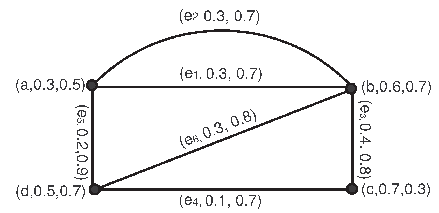
An important trivial class of PFM is Pythagorean fuzzy cycle matroid $\mathcal{PM}(G^{\prime })$ associated with graph $G^{\prime }$(Definition 11). The set $\mathcal{A}$ is the family of edge subsets of $E^{\prime }$($\xi \subseteq E^{\prime }$) with $supp(\xi )$ not containing a cycle of $G^{\prime }$. In other words, the members of $\mathcal{A}$ are Pythagorean fuzzy subgraphs ξ of $G^{\prime }$ whose $supp(\xi )$ is a forest and hence from Definition 16$\mathcal{PM}(G^{\prime })$ is matroid.

Consider a graph $G=(V,E)$ with vertex set $V=\{a,b,c,d\}$ and edge set $E=\{e_1=ab,e_2=ba,e_3=bc,e_4=cd,e_5=ad,e_6=bd\}\subseteq V\times V$. Let $V^{\prime } and E^{\prime }$ be PFSs in $V and E$ respectively and defined as,

$V^{\prime }=\{(a,0.3,0.5),(b,0.6,0.7),(c,0.7,0.3),(d,0.5,0.7)\},$

$E^{\prime }=\{(e_1,0.3,0.7),(e_2,0.3,0.7),(e_3,0.4,0.8),(e_4,0.1,0.7),(e_5,0.2,0.9),(e_6,0.3,0.8)\}.$

Then from Definition 11, $G^{\prime }$ ia a PFG of G in Figure 1 and $\mathcal{PM}(G^{\prime })$ is a Pythagorean fuzzy cycle matroid.

$\mathcal{A}=\{\xi \mid \xi \subseteq E^{\prime }, supp(\xi ) is not an edge set of cycle\}.$

${\mathcal{A}}_r(G^{\prime })=\{\{(e_1,0.3,0.7),(e_2,0.3,0.7)\},\{(e_1,0.3,0.7),(e_5,0.2,0.9),(e_6,0.3,0.8)\},\{(e_2,0.3,0.7),(e_5,0.2,0.9),(e_6,0.3,0.8)\},\{(e_3,0.4,0.8),(e_4,0.1,0.7),(e_6,0.3,0.8)\},\{(e_1,0.3,0.7),(e_3,0.4,0.8),(e_4,0.1,0.7),(e_5,0.2,0.9)\},\{(e_2,0.3,0.7),(e_3,0.4,0.8),(e_4,0.1,0.7),(e_5,0.2,0.9)\}\}.$

$\mathcal{B}(\mathcal{PM})=\{\{(e_1,0.3,0.7),(e_3,0.4,0.8),(e_4,0.1,0.7)\},\{(e_1,0.3,0.7),(e_3,0.4,0.8),(e_5,0.2,0.9)\},\{(e_1,0.3,0.7),(e_3,0.4,0.8),(e_6,0.3,0.8)\},\{(e_1,0.3,0.7),(e_4,0.1,0.7),(e_5,0.2,0.9)\},\{(e_1,0.3,0.7),(e_4,0.1,0.7),(e_6,0.3,0.8)\},\{(e_2,0.3,0.7),(e_3,0.4,0.8),(e_4,0.1,0.7)\},\{(e_2,0.3,0.7),(e_3,0.4,0.8),(e_5,0.2,0.9)\},\{(e_2,0.3,0.7),(e_3,0.4,0.8),(e_6,0.3,0.8)\},\{(e_2,0.3,0.7),(e_4,0.1,0.7),(e_5,0.2,0.9)\},\{(e_2,0.3,0.7),(e_4,0.1,0.7),(e_6,0.3,0.8)\},\{(e_3,0.4,0.8),(e_4,0.1,0.7),(e_5,0.2,0.9)\},\{(e_3,0.4,0.8),(e_5,0.2,0.9),(e_6,0.3,0.8)\},\{(e_4,0.1,0.7),(e_5,0.2,0.9),(e_6,0.3,0.8)\}\}.$

For $\xi =\{(e_3,0.4,0.6),(e_4,0.7,0.1),(e_5,0.2,0.3)\}$, ${\mu }_r(\xi )=(1.3,1.0).$

2.

A very basic example for which we have is,

$$\mathcal{A}=\{\xi \in \mathcal{P}(X):\mid supp(\xi )\mid \le k\}.$$

and for any positive integer k with $k\le n$ and $\mid X\mid =n$, the matroid is denoted by ${\mathcal{U}}_n^k$ and called Pythagorean fuzzy uniform matroid. The Pythagorean fuzzy circuits of ${\mathcal{U}}_n^k$ are all PFSs of X with size $k+1$ and bases are exactly the sets of size k.

For this, we consider the following Pythagorean fuzzy uniform matroid $\mathcal{PM}={\mathcal{U}}_n^k$ with the set $X=\{a_1,a_2,a_3,a_4\}$ and $\mathcal{A}=\{\xi \in \mathcal{P}(X):\mid supp(\xi )\mid \le 2\}$. For all $y\in X$ and for any $\xi \in \mathcal{P}(X)$, define $\xi (y)=\lambda (y)$ as,

$$\lambda (y)=\left\{\begin{array}{cc}(0.3,0.2),\hfill & y=a_1,\hfill \\ \left(0.4,0.6\right),\hfill & y=a_2,\hfill \\ (0.1,0.3),\hfill & y=a_3,\hfill \\ (0.6,0.3),\hfill & y=a_4.\hfill \end{array}\right.$$

$\mathcal{A}=\{\varnothing ,\{(a_1,0.3,0.2)\},\{(a_2,0.4,0.6)\},\{(a_3,0.1,0.3)\},\{(a_4,0.6,0.3)\},\{(a_1,0.3,0.2),(a_2,0.4,0.6)\},\{(a_1,0.3,0.4),(a_3,0.1,0.3)\},\{(a_1,0.3,0.2),(a_4,0.6,0.3)\},\{(a_2,0.4,0.6),(a_3,0.1,0.3)\},\{(a_2,0.4,0.6),(a_4,0.6,0.3)\},\{(a_3,0.1,0.3),(a_4,0.6,0.3)\}\}.$

The family of all Pythagorean fuzzy circuits is,

${\mathcal{A}}_r(\mathcal{PM})=\{\{(a_1,0.3,0.2),(a_2,0.4,0.6),(a_3,0.1,0.3)\},\{(a_1,0.3,0.2),(a_2,0.4,0.6),(a_4,0.6,0.3)\},\{(a_1,0.3,0.2),(a_3,0.1,0.3),(a_4,0.6,0.3)\},\{(a_2,0.4,0.6),(a_3,0.1,0.3),(a_4,0.6,0.3)\}\}$.

$\mathcal{B}(\mathcal{PM})=\{\{(a_1,0.3,0.2),(a_2,0.4,0.6)\},\{(a_1,0.3,0.4),(a_3,0.1,0.3)\},\{(a_1,0.3,0.2),(a_4,0.6,0.3)\},\{(a_2,0.4,0.6),(a_3,0.1,0.3)\},\{(a_2,0.4,0.6),(a_4,0.6,0.3)\},\{(a_3,0.1,0.3),(a_4,0.6,0.3)\}\}.$

For $\xi =\{(a_1,0.3,0.2),(a_2,0.4,0.6)\},{\mu }_r(\xi )=(0.7,0.8)$.

Proposition 4.

If $\mathcal{PM}(G^{\prime })$ is a Pythagorean fuzzy cycle matroid and ${\mathcal{A}}_r$ is the collection of Pythagorean fuzzy edge subsets whose support is exactly the edge set of any cycle in $G^{\prime }$. Then ${\mathcal{A}}_r$ is the collection of Pythagorean fuzzy circuits of $\mathcal{PM}(G^{\prime })$.

Proof. 

This result is the direct consequence of Example 3 (Part 1). □

Definition 20.

Let $l_1=(l_1^{\prime },s_1^{\prime }), l_2=(l_2^{\prime },s_2^{\prime }),\dots ,l_n=(l_n^{\prime },s_n^{\prime })$ be ‘n’ PFNs with order $l_1^{\prime }\le l_2^{\prime }{\le }_3^{\prime }\le \dots \le l_n^{\prime }$ and $s_1^{\prime }\ge s_2^{\prime }\ge s_3^{\prime }\ge \dots \ge s_n^{\prime }$. Then for each $1\le i\le n$, the pair $l_i=(l_i^{\prime },s_i^{\prime })$ satisfies the following condition,

$$l_i\le l_{i+1}⟺l_i^{\prime }\le l_{i+1}^{\prime } and s_i^{\prime }\ge s_{i+1}^{\prime }.$$

In this work, sometimes we use l instead of $l=(l^{\prime },s^{\prime })$ and $\mathbf{0}\le l\le \mathbf{1}$, where $\mathbf{0}=(0,1)$ and $\mathbf{1}=(1,0)$ with $\mathcal{S}(\mathbf{0})=0 and \mathcal{S}(\mathbf{1})=1$ respectively.

Definition 21.

If $\mathbf{0}<l\le \mathbf{1}$, then $l-cut$ for PFS $\xi \in \mathcal{P}(X)$ is defined as,

$${\mathcal{A}}_l(\xi )=\{x\in X:{\xi }^P(x)\ge l^{\prime } and {\xi }^N(x)\le s^{\prime }\}.$$

Theorem 1.

Let $\mathcal{PM}=(X,\mathcal{A})$ be a PFM, and for each $\mathbf{0}<l\le \mathbf{1}$, define ${\mathcal{A}}_l=\{{\mathcal{A}}_l(\xi )\mid \xi \in \mathcal{A}\}$. Then ${\mathcal{M}}_l=(X,{\mathcal{A}}_l)$ is a matroid on X.

Proof. 

The first condition of Definition 1 is obvious. To prove condition 2, for any ${\xi }_1\in \mathcal{A}$, assume that ${\mathcal{A}}_l({\xi }_1)\in {\mathcal{A}}_l and \gamma \subseteq {\mathcal{A}}_l({\xi }_1)$. Let ${\xi }_2\in \mathcal{P}(X)$ be a PFS, we define,

$${\xi }_2(y)=\left\{\begin{array}{cc}(l^{\prime },s^{\prime })\hfill & y\in \gamma ,\hfill \\ (0,1)\hfill & otherwise.\hfill \end{array}\right.$$

where $0<{(l^{\prime })}^2+{(s^{\prime })}^2\le 1$ with $\mathcal{S}(l^{\prime },s^{\prime })>0$. This implies that ${\xi }_2\subseteq {\xi }_1,{\xi }_2\in \mathcal{A} and {\mathcal{A}}_l({\xi }_2)=\gamma , that gives\gamma \in {\mathcal{A}}_l$. To prove condition 3, for any ${\xi }_1,{\xi }_2\in \mathcal{A}$, let ${\mathcal{A}}_l({\xi }_1),{\mathcal{A}}_l({\xi }_2)\in {\mathcal{A}}_l with\mid {\mathcal{A}}_l({\xi }_1)\mid <\mid {\mathcal{A}}_l({\xi }_2)\mid$. Define $\widehat{{\xi }_1} and \widehat{{\xi }_2}$ by,

$$\widehat{{\xi }_1}(y)=\left\{\begin{array}{cc}(l^{\prime },s^{\prime })\hfill & y\in {\mathcal{A}}_l({\xi }_1),\hfill \\ (0,1)\hfill & otherwise.\hfill \end{array}\right.$$

$$\widehat{{\xi }_2}(y)=\left\{\begin{array}{cc}(l^{\prime },s^{\prime })\hfill & y\in {\mathcal{A}}_l({\xi }_2),\hfill \\ (0,1)\hfill & otherwise.\hfill \end{array}\right.$$

where $0<{(l^{\prime })}^2+{(s^{\prime })}^2\le 1$ with $\mathcal{S}(l^{\prime },s^{\prime })>0$. It is observed that $\mid supp(\widehat{{\xi }_1})\mid <\mid supp(\widehat{{\xi }_2})\mid$. Since $\mathcal{PM}$ is a PFM and $\widehat{{\xi }_1},\widehat{{\xi }_2}\in \mathcal{A}$, then there exists $\omega \in \mathcal{A}$ such that $\widehat{{\xi }_1}\subset \omega \subseteq \widehat{{\xi }_1}\cup \widehat{{\xi }_2}$ and $m(\omega )\ge min\{m(\widehat{\widehat{{\xi }_1}}),m(\widehat{{\xi }_2})\}$. Since,

$$(\widehat{{\xi }_1}\cup \widehat{{\xi }_2})(y)=\left\{\begin{array}{cc}(l^{\prime },s^{\prime })\hfill & y\in {\mathcal{A}}_l({\xi }_1)\cup {\mathcal{A}}_l({\xi }_2),\hfill \\ (0,1)\hfill & otherwise.\hfill \end{array}\right.$$

where $0\le {(l^{\prime })}^2+{(s^{\prime })}^2\le 1$ with $\mathcal{S}(l^{\prime },s^{\prime })>0$. Then there is a set ${\mathcal{A}}_l({\xi }_3)$ with ${\mathcal{A}}_l({\xi }_1)\subset {\mathcal{A}}_l({\xi }_3)\subseteq {\mathcal{A}}_l({\xi }_1)\cup {\mathcal{A}}_l({\xi }_2)$, and $\omega$ is defined as,

$$\omega (y)=\left\{\begin{array}{cc}(l^{\prime },s^{\prime })\hfill & y\in {\mathcal{A}}_l({\xi }_3),\hfill \\ (0,1)\hfill & otherwise.\hfill \end{array}\right.$$

where $0<{(l^{\prime })}^2+{(s^{\prime })}^2\le 1$ with $\mathcal{S}(l^{\prime },s^{\prime })>0$. Since ${\mathcal{A}}_l({\xi }_3) \in {\mathcal{A}}_l$, hence ${\mathcal{M}}_l$ is a matroid on X. □

Example 4.

From Example 3 (Part 2), consider a Pythagorean fuzzy uniform matroid $\mathcal{PM}={\mathcal{U}}_n^k$ with the collection of independent sets $\mathcal{A}$.

Take $l^{\prime }=0.1$ and $s^{\prime }=0.4$ and we write $l=(0.1,0.4)$ then,

$${\mathcal{A}}_l=\{\varphi ,\{a_1\},\{a_3\},\{a_4\},\{a_1,e_3\},\{a_1,e_4\},\{a_3,a_4\}\}.$$

Clearly, the pair $(X,{\mathcal{A}}_l)$ is a crisp matroid and follows that the pair $(X,{\mathcal{A}}_l)$ is a crisp matroid for every $\mathbf{0}<l\le \mathbf{1}$.

Corollary 1.

Let $\mathcal{PM}=(X,\mathcal{A})$ be a PFM and let for each $\mathbf{0}<l\le \mathbf{1},$${\mathcal{M}}_l=(X,{\mathcal{A}}_l)$ be the matroid on X (Theorem 1). Since X is finite, therefore for finite number of matroids, we have a finite sequence $\mathbf{0}<l_1<l_2<\dots <l_n$ such that,

1.

$l_0=\mathbf{0},l_n\le \mathbf{1}$,

2.

${\mathcal{A}}_{\alpha }\ne \varphi if \mathbf{0}<\alpha \le l_n and {\mathcal{A}}_{\alpha }=\varphi if \alpha >l_n$,

3.

If $l_i<q,r<l_{i+1}, then {\mathcal{A}}_q={\mathcal{A}}_r,0\le i\le n-1$,

4.

If $l_i<q<l_{i+1}<r<l_{i+2}, then {\mathcal{A}}_q\supset {\mathcal{A}}_r,0\le i\le n-2$.

The sequence $l_0=\mathbf{0},l_1,l_2,\dots ,l_n$ is known as a fundamental sequence of $\mathcal{PM}$. From observation 4 of Corollary 1, let $\overline{l_i}=\frac{1}{2}(l_{i-1}+l_i) for 1\le i\le n$, then ${\mathcal{M}}_{{\overline{l}}_1}\supset {\mathcal{M}}_{{\overline{l}}_2}\supset \dots \supset {\mathcal{M}}_{{\overline{l}}_n}$ is called a $\mathcal{M}$-induced matroid sequence.

Theorem 2.

Let $(X,{\mathcal{A}}_{l_1}),(X,{\mathcal{A}}_{l_2}),\dots ,(X,{\mathcal{A}}_{l_n})$ be a sequence of crisp matroids with finite sequence $\mathbf{0}=l_0<l_1<l_2<\dots <l_n\le \mathbf{1}$. We assume that for each l, ${\mathcal{A}}_l={\mathcal{A}}_{l_i} and {\mathcal{A}}_l=\varphi if l_n<l\le \mathbf{1}$, where $l_{i-1}<l\le l_i$$(i=1,2,\dots ,n)$, define,

$$\widehat{\mathcal{A}}=\{\xi \in \mathcal{P}(X)\mid {\mathcal{A}}_l(\xi )\in {\mathcal{A}}_l,\mathbf{0}<l\le \mathbf{1}\}.$$

Then $(X,\widehat{\mathcal{A}})$ is a PFM.

Proof. 

It is clear that $\varphi \in \widehat{\mathcal{A}}$. To prove the second condition of Definition 16, let ${\xi }_1\in \widehat{\mathcal{A}},{\xi }_2\in \mathcal{P}(X)$, and ${\xi }_2\subseteq {\xi }_1.$ As seen from definition of $\widehat{\mathcal{A}},$ we have ${\mathcal{A}}_l({\xi }_1)\in {\mathcal{A}}_l,$ for each l, ${\mathcal{A}}_l({\xi }_2)\subseteq {\mathcal{A}}_l({\xi }_1)$ and given that $(X,{\mathcal{A}}_l)$ is a crisp matroid, so ${\mathcal{A}}_l({\xi }_2)\in {\mathcal{A}}_l$ and gives ${\xi }_2\in \widehat{\mathcal{A}}$.

Now, to prove condition 3 of Definition 16, for ${\xi }_1,{\xi }_2\in \widehat{\mathcal{A}}$ with $\mid supp({\xi }_2)\mid <\mid supp({\xi }_1)\mid$ we define a PFN,

$$\zeta =min\{m({\xi }_1),m({\xi }_2)\}, where m({\xi }_i)=inf\{{\xi }_i(x):x\in supp({\xi }_i)\}.$$

Observe that $supp({\xi }_1),supp({\xi }_2)\in {\mathcal{A}}_{\zeta }$. As ${\mathcal{A}}_{\zeta }$ is a collection of independent sets, then there is a subset $W\in {\mathcal{A}}_{\zeta }$, which is also independent, with $supp({\xi }_2)\subset W\subseteq supp({\xi }_1)\cup supp({\xi }_2)$.

Let,

$${\xi }_3(y)=\left\{\begin{array}{cc}{\xi }_2(y)\hfill & y\in supp({\xi }_2),\hfill \\ \zeta \hfill & y\in W-\{supp({\xi }_2)\},\hfill \\ (0,1)\hfill & otherwise.\hfill \end{array}\right.$$

Then it is clear from Definition 16, PFS ${\xi }_3$ satisfies third condition, and hence $(X,\widehat{\mathcal{A}})$ is a PFM. □

Theorem 3.

Let $\mathcal{PM}=(X,\mathcal{A})$ be a PFM and for each $\mathbf{0}<l\le \mathbf{1}, {\mathcal{M}}_l=(X,{\mathcal{A}}_l)$ be a matroid (Theorem 1). Let $\widehat{\mathcal{A}}=\{\xi \in \mathcal{P}(X)\mid {\mathcal{A}}_l(\xi )\in {\mathcal{A}}_l,\mathbf{0}<l\le \mathbf{1}\}. Then \mathcal{A}=\widehat{\mathcal{A}}$.

Proof. 

It is easily seen that $\mathcal{A}\subseteq \widehat{\mathcal{A}}$. To prove the other side $\widehat{\mathcal{A}}\subseteq \mathcal{A}$, we establish the following steps.

Consider a non-zero Pythagorean fuzzy range $\{{\sigma }_1,{\sigma }_2,\dots ,{\sigma }_r\}$ of $\xi \in \widehat{\mathcal{A}}$, where ${\sigma }_i=({\sigma }_i^{*},{\sigma }_i^{\prime })$ and with order ${\sigma }_1>{\sigma }_2>\dots >{\sigma }_r>\mathbf{0}$ (see Definition 20). For each $1\le i\le r,{\mathcal{A}}_{{\sigma }_i}(\xi )\in {\mathcal{A}}_{{\sigma }_i}$ and from Corollary 1, for $1\le i\le r-1,{\mathcal{A}}_{{\sigma }_i}(\xi )\subset {\mathcal{A}}_{{\sigma }_{i+1}}(\xi )$. Define ${\varphi }_i\in \mathcal{P}(X)$ for each $1\le i\le r$ as

$${\varphi }_i(y)=\left\{\begin{array}{cc}({\sigma }_i^{*},{\sigma }_i^{\prime })\hfill & ify\in {\mathcal{A}}_{{\sigma }_i}(\xi ),\hfill \\ (0,1)\hfill & otherwise.\hfill \end{array}\right.$$

where $0<{({\sigma }_i^{*})}^2+{({\sigma }_i^{\prime })}^2\le 1$. As we have ${\mathcal{A}}_{{\sigma }_i}(\xi )\in {\mathcal{A}}_{{\sigma }_i}$, which implies that ${\varphi }_i\in \mathcal{A}$ with ${\cup }_{i=1}^r{\varphi }_i=\xi$. We use an induction method to prove $\xi \in \mathcal{A}$ and for each $1\le i\le r$, $supp({\varphi }_i)=\{y_1,y_2,\dots ,y_{n_i}\}$, assume that $supp(\xi )=\{y_1,y_2,\dots ,y_{n_r}\}$. Since ${\varphi }_1\in \mathcal{A}$ therefore, it is adequate to show that if for $k-1<r$, ${\cup }_{i=1}^{k-1}{\varphi }_i\in \mathcal{A}$, then ${\cup }_{i=1}^k{\varphi }_i\in \mathcal{A}$, for each $k<r$. Define a set,

$${\psi }_1(y)=\left\{\begin{array}{cc}({\sigma }_k^{*},{\sigma }_k^{\prime })\hfill & ify\in \{y_1,y_2,\dots ,y_{n_{k-1}+1}\},\hfill \\ (0,1)\hfill & otherwise.\hfill \end{array}\right.$$

It can be seen that for each $1<i<k-1,{\sigma }_k<{\sigma }_i$ therefore, ${\psi }_1\subset {\varphi }_k$ which gives that ${\psi }_1\in \mathcal{A}$. Define ${\mathsf{\Psi }}_1\in \mathcal{P}(X)$ by,

$${\mathsf{\Psi }}_1(y)=\left\{\begin{array}{cc}\xi (y_{n_{k-1}+1})=({\sigma }_k^{*},{\sigma }_k^{\prime })\hfill & ify=y_{n_{k-1}+1,}\hfill \\ (0,1)\hfill & otherwise.\hfill \end{array}\right.$$

Since by induction method ${\cup }_{i=1}^{k-1}{\varphi }_i\in \mathcal{A}$ and $supp({\cup }_{i=1}^{k-1}{\varphi }_i)=\{y_1,y_2,\dots ,y_{n_{k-1}}\}$, $m({\cup }_{i=1}^{k-1}{\varphi }_i)>{\sigma }_k$ therefore, condition 3 of Definition 16 implies that ${\cup }_{i=1}^{k-1}{\varphi }_i\cup {\mathsf{\Psi }}_1\in \mathcal{A}$. If $n_{k-1}+1=n_k ,then {\cup }_{i=1}^k{\varphi }_i\in \mathcal{A}$ and we are done. But on the other hand, if $n_{k-1}+1<n_k$ then define,

$${\psi }_2(y)=\left\{\begin{array}{cc}({\sigma }_k^{*},{\sigma }_k^{\prime })\hfill & ify\in \{y_1,y_2,\dots ,y_{n_{k-1}+1},y_{n_{k-1}+2}\},\hfill \\ (0,1)\hfill & otherwise.\hfill \end{array}\right.$$

Since for each $1<i<k-1$, we have $({\sigma }_k^{*},{\sigma }_k^{\prime })<({\sigma }_i^{*},{\sigma }_i^{\prime })$ (see Definition 20), therefore ${\psi }_2\subset {\varphi }_k$ which implies that ${\psi }_2\in \mathcal{A}$. Now define ${\mathsf{\Psi }}_2\in \mathcal{P}(X)$ by,

$${\mathsf{\Psi }}_2(y)=\left\{\begin{array}{cc}\xi (y_{n_{k-1}+2})=({\sigma }_k^{*},{\sigma }_k^{\prime })\hfill & ify=y_{n_{k-1}+2,}\hfill \\ (0,1)\hfill & otherwise.\hfill \end{array}\right.$$

Since $supp({\cup }_{i=1}^{k-1}{\varphi }_i\cup {\mathsf{\Psi }}_1)=\{y_1,y_2,\dots ,y_{n_{k-1}+1}\}$, $m({\cup }_{i=1}^{k-1}{\varphi }_i\cup {\mathsf{\Psi }}_1)>{\sigma }_k$, therefore from Definition 16, ${\cup }_{i=1}^{k-1}{\varphi }_i\cup {\mathsf{\Psi }}_1\cup {\mathsf{\Psi }}_2\in \mathcal{A}$. If $n_{k-1}+2=n_k then {\cup }_{i=1}^k{\varphi }_i\in \mathcal{A}$ and it is finished. If $n_{k-1}+2<n_k$ then we proceed with the induction procedure and get a PFS ${\tau }_j={\cup }_{i=1}^{k-1}{\varphi }_i\cup {\mathsf{\Psi }}_1\cup {\mathsf{\Psi }}_2\cup ,\dots \cup {\mathsf{\Psi }}_n$ with ${\tau }_j={\cup }_{i=1}^k{\varphi }_i$ which completes the proof. □

Definition 22.

Let $l_0,l_1,\dots ,l_n$ be the fundamental sequence of a PFM. For any Pythagorean fuzzy pair $l,\mathbf{0}<l\le \mathbf{1}, define \overline{{\mathcal{A}}_l}={\mathcal{A}}_{\overline{l_i}} where ,l_{i-1}<l\le l_i and \overline{l_i}=\frac{1}{2}(l_{i-1}+l_i)$. If $l>l_n take \overline{{\mathcal{A}}_l}={\mathcal{A}}_l.$ Define,

$$\overline{\mathcal{A}}=\{\xi \in \mathcal{P}(X)\mid {\mathcal{A}}_l(\xi )\in \overline{{\mathcal{A}}_l}, for each \mathbf{0}<l\le \mathbf{1}\}.$$

Then $\overline{\mathcal{PM}}=(X,\overline{\mathcal{A}})$ is called closure of $\mathcal{PM}=(X,\mathcal{A})$.

It can be observed directly from Theorem 2 that $\overline{\mathcal{PM}}$ is also PFM.

Definition 23.

Let $\mathcal{PM}=(X,\mathcal{A})$ be a PFM with fundamental sequence $l_0<l_1<l_2<\dots <l_n\le \mathbf{1}$ and $\mathcal{PM}$ is called closed a matroid if, for $l_i<l\le l_{i+1}(i=1,2,3,\dots ,n-1)$ we have ${\mathcal{A}}_l={\mathcal{A}}_{l_{i+1}}$.

Example 5.

Let $X=\{1,2,3,4\}$ and assume that,

${\mathcal{A}}_1=\{\varphi ,\{1\},\{2\},\{4\},\{2,4\}\}$,

${\mathcal{A}}_{\frac{2}{3}}=\{\varphi ,\{1\},\{2\},\{3\},\{4\},\{1,4\},\{2,4\}\}$, and

${\mathcal{A}}_{\frac{1}{2}}=\{\varphi ,\{1\},\{2\},\{3\},\{4\},\{1,4\},\{2,3\},\{2,4\}\}$.

Then $(X,{\mathcal{A}}_1)$, $(X,{\mathcal{A}}_{\frac{2}{3}})$, and $(X,{\mathcal{A}}_{\frac{1}{2}})$ are matroids respectively, such that ${\mathcal{A}}_1\subset {\mathcal{A}}_{\frac{2}{3}}\subset {\mathcal{A}}_{\frac{1}{2}}$. For each $l=(l^{\prime },s^{\prime })$ with $0\le {(l^{\prime })}^2+{(s^{\prime })}^2\le 1$ we define,

$${\mathcal{A}}_l=\{\begin{array}{cc}{\mathcal{A}}_{\frac{1}{2}}& \mathit{if} (0,1)<l\le (\frac{1}{2},0),\\ {\mathcal{A}}_{\frac{2}{3}}& \mathit{if} (\frac{1}{2},1)<l\le (\frac{2}{3},0),\\ {\mathcal{A}}_1& \mathit{if} (\frac{2}{3},1)<l\le (1,0).\end{array}$$

and

$$\mathcal{A}=\{\xi \in \mathcal{P}(X)\mid {\mathcal{A}}_l(\xi )\in {\mathcal{A}}_l,\mathbf{0}<l\le \mathbf{1}\}.$$

Hence the pair $(X,\mathcal{A})$ is closed PFM having fundamental sequence $l_0=(0,1),l_1=(\frac{1}{2},0),l_2=(\frac{2}{3},0),l_3=(1,0).$

Lemma 1.

Let ${\mu }_r$ and $\overline{{\mu }_r}$ be Pythagorean fuzzy rank functions of $\mathcal{PM}$ and its closure $\overline{\mathcal{PM}}$ respectively. Then $\overline{{\mu }_r}={\mu }_r$.

Proof. 

It follows from Definition 22 that $\mathcal{A}\subseteq \overline{\mathcal{A}}$ and for each $\xi \in \mathcal{P}(X)$, ${\mu }_r(\xi )\le \overline{{\mu }_r}(\xi )$. To prove $\overline{{\mu }_r}(\xi )\le {\mu }_r(\xi )$, suppose that ${\xi }_i\subseteq \xi$, where ${\xi }_i\in \overline{\mathcal{A}}.$ Consider a Pythagorean fuzzy range $\mathbf{0}<{\sigma }_1<{\sigma }_2<\dots <{\sigma }_r$ of ${\xi }_i$. Let $\delta >\mathbf{0}$ and define,

$${\delta }^{\prime }=min\left\{\delta , \underset{1\le j\le r-1}{min}\{\frac{1}{2}({\sigma }_j+{\sigma }_{j+1})\}\right\}.$$

Let $\{l_0,l_1,\dots ,l_n\}$ be the set of fundamental sequence of $\mathcal{PM}$. We define,

$${{\xi }_i}^{\prime }(x)=\left\{\begin{array}{cc}{\xi }_i(x)\hfill & if{\xi }_i(x)\notin \{l_0,l_1,\dots ,l_n\},\hfill \\ {\xi }_i(x)/{\delta }^{\prime }\hfill & if{\xi }_i(x)\in \{l_0,l_1,\dots ,l_n\}.\hfill \end{array}\right.$$

It is easy to see that ${{\xi }_i}^{\prime }\in \mathcal{A}$ and from Definition 19, $\mid {\xi }_i^{\prime }\mid \le \mid {\xi }_i\mid \le \mid {\xi }_i^{\prime }\mid +\delta$. Now, let $\{{\xi }_{i_k}\}\subseteq \overline{\mathcal{A}}$ such that for each k, ${\xi }_{i_k}\subseteq \xi$ with ${lim}_{k\to \infty }\mid {\xi }_{i_k}\mid =\overline{{\mu }_r}(\xi )$. So, there exists ${\xi }_{i_k}^{\prime }\in \mathcal{A}$ with $\mid {\xi }_{i_k}\mid <\mid {\xi }_{i_k}^{\prime }\mid +\delta$. Then we have,

$${\mu }_r(\xi )<sup\{{\xi }_{i_k}^{\prime }\}+\delta .$$

As $\delta >\mathbf{0}$ is an arbitrary Pythagorean fuzzy number and hence, we have $\overline{{\mu }_r}(\xi )\le {\mu }_r(\xi )$. □

Suppose ${\mu }_r$ is a rank function for $\mathcal{PM}=(X,\mathcal{A})$ with fundamental sequence $l_0,l_1,\dots ,l_n$. We define a new function $\widehat{{\mu }_r}:\mathcal{P}(X)\to {[0,\infty )}^2$ which is submodular. This function helps to show that ${\mu }_r$ is submodular. Here, we need a useful construction to define this new function.

For any $\xi \in \mathcal{P}(X)$, assume a Pythagorean fuzzy range $\mathbf{0}<{\sigma }_1<{\sigma }_2<\dots <{\sigma }_r$. Consider a common refinement ${\gamma }_1<{\gamma }_2<\dots <{\gamma }_s$ of $l_i^{\prime }s$ and ${\sigma }_j^{\prime }s$ i.e.,

$$\{{\gamma }_1,{\gamma }_2,\dots ,{\gamma }_s\}=\{{\sigma }_1,{\sigma }_2,\dots ,{\sigma }_r\}\cup \{l_1,l_2,\dots ,l_n\}.$$

Since, for each $0\le i\le n$, ${\mathcal{M}}_{l_i}=(X,{\mathcal{A}}_{l_i})$ is a crisp matroid with the rank function ${\mathcal{R}}_i$. There exists an integer i for each k with $l_{i-1}\le {\gamma }_{k-1}<{\gamma }_k\le l_i$. We define for each correspondence pair $(i,k)$,

$${\eta }_k(\xi )=\left\{\begin{array}{cc}({\gamma }_k-{\gamma }_{k-i}){\mathcal{R}}_i({\mathcal{A}}_{{\gamma }_k}(\xi ))\hfill & if{\gamma }_k\le l_n,\hfill \\ (0,1)\hfill & if{\gamma }_k>l_n.\hfill \end{array}\right.$$

In addition, for each $1\le k\le s$, and ${\gamma }_{k-1}\le \nu \le {\gamma }_k$ we have ${\mathcal{A}}_{\nu }(\xi )={\mathcal{A}}_{{\gamma }_k}(\xi )$. Then a new mapping $\widehat{{\mu }_r}:\mathcal{P}(X)\to {[0,\infty )}^2$ defined as,

$$\widehat{{\mu }_r}=\sum _{k=1}^s{\eta }_k(\xi ).$$

(1)

Lemma 2.

Let $\{{\gamma }_1,{\gamma }_2,\dots ,{\gamma }_s\}\subseteq \{{\theta }_1,{\theta }_2,\dots ,{\theta }_p\}$ with $\mathbf{0}<{\theta }_1<{\theta }_2<\dots <{\theta }_p$. The pair $(i,t)$ is the correspondence pair, for each $1\le i\le n$, if $l_{i-1}\le {\theta }_{t-1}<{\theta }_t\le l_i$. Let us define a function ${\eta }_t^{*}:\mathcal{P}(X)\to {\mathbb{R}}^2,$ for each correspondence pair $(i,t)$, as,

$${\eta }_t^{*}(\xi )=\left\{\begin{array}{cc}({\theta }_t-{\theta }_{t-i})R_i({\mathcal{A}}_{{\theta }_t}(\xi ))\hfill & if{\theta }_t\le l_n,\hfill \\ (0,1)\hfill & if{\theta }_t>l_n.\hfill \end{array}\right.$$

Then ${\sum }_{k=1}^s{\eta }_k(\xi )={\sum }_{t=1}^p{\eta }_t^{*}(\xi ).$

Proof. 

The proof is straightforward from the construction of Equation (1). □

Theorem 4.

Let $\mathcal{PM}=(X,\mathcal{A})$ be a PFM with fundamental sequence $l_0,l_1,\dots ,l_n$ and $\widehat{{\mu }_r}$ defined by Equation (1). The $\widehat{{\mu }_r}$ is submodular.

Proof. 

Let ${\xi }_1$ and ${\xi }_2$ be two PFSs in $\mathcal{P}(X)$. Consider $\{{\sigma }_1,{\sigma }_2,\dots ,{\sigma }_s\}$ and $\{{\gamma }_1,{\gamma }_2,\dots ,{\gamma }_t\}$ be the non-zero Pythagorean fuzzy ranges of ${\xi }_1$ and ${\xi }_2$, respectively. Take a common refinement as above,

$$\{{\theta }_1,{\theta }_2,\dots ,{\theta }_u\}=\{{\sigma }_1,{\sigma }_2,\dots ,{\sigma }_s\}\cup \{{\gamma }_1,{\gamma }_2,\dots ,{\gamma }_t\}\cup \{l_0,l_1,\dots ,l_n\}.$$

From Lemma 2 we have $\widehat{{\mu }_r}={\sum }_{k=1}^u{\eta }_k^{*}(\xi ).$ Since for each k, ${\theta }_{k-1}<{\theta }_k$ which means ${\theta }_k-{\theta }_{k-1}>\mathbf{0}$ and from submodularity of the crisp rank function $R_i$,

$$\begin{array}{c}\hfill \begin{array}{cc}\hfill \sum _{k=1}^u({\theta }_k-{\theta }_{k-1})R_i({\mathcal{A}}_{{\theta }_k}({\xi }_1))& +\sum _{k=1}^u({\theta }_k-{\theta }_{k-1})R_i({\mathcal{A}}_{{\gamma }_k}({\xi }_2))\hfill \\ & \ge \sum _{k=1}^u({\theta }_k-{\theta }_{k-1})R_i({\mathcal{A}}_{{\gamma }_k}({\xi }_1)\cup {\mathcal{A}}_{{\gamma }_k}({\xi }_2))\hfill \\ & +\sum _{k=1}^u({\theta }_k-{\theta }_{k-1})R_i({\mathcal{A}}_{{\gamma }_k}({\xi }_1)\cap {\mathcal{A}}_{{\gamma }_k}(\xi )).\hfill \end{array}\end{array}$$

(2)

Which gives that $\widehat{{\mu }_r}({\xi }_1)+\widehat{{\mu }_r}({\xi }_2)\ge \widehat{{\mu }_r}({\xi }_1\cup {\xi }_2)+\widehat{{\mu }_r}({\xi }_1\cap {\xi }_2).$ □

Theorem 5.

Let $\mathcal{PM}=(X,\mathcal{A})$ be PFM, then ${\mu }_r=\widehat{{\mu }_r}.$

Proof. 

Assume that $\mathcal{PM}$ is closed, then from Lemma 1, ${\mu }_r=\overline{{\mu }_r}$ and ${\mu }_r({\xi }_1)\ne (0,0)$ for some ${\xi }_1\in \mathcal{P}(X)$. Let ${\xi }_2\in \mathcal{A}$ with ${\xi }_2\subseteq {\xi }_1$ such that ${\mu }_r({\xi }_1)=\mid {\xi }_2\mid$. We need to show that $\widehat{{\mu }_r}({\xi }_1)={\mu }_r({\xi }_1)$.

Assume a non-zero Pythagorean fuzzy range $\mathbf{0}<{\sigma }_1<{\sigma }_2<\dots <{\sigma }_r$. Consider a common refinement ${\gamma }_1<{\gamma }_2<\dots <{\gamma }_s$ of $l_i^{\prime }s$ and ${\sigma }_j^{\prime }s$ i.e.,

$$\{{\gamma }_1,{\gamma }_2,\dots ,{\gamma }_s\}=\{{\sigma }_1,{\sigma }_2,\dots ,{\sigma }_r\}\cup \{l_1,l_2,\dots ,l_n\}.$$

where $l_0<l_1<\dots <l_n$ is the fundamental sequence of $\mathcal{PM}$ and ${\gamma }_{i_j}=l_j$, $1\le j\le n$. For each $0<\alpha \le 1$, let,

$${\mathcal{A}}_{\alpha }^{{\xi }_1}=\{A\in {\mathcal{A}}_{\alpha }:A\subseteq {\mathcal{A}}_{\alpha }({\xi }_1)\}, and {\alpha }^{*}=sup\{\alpha :{\mathcal{A}}_{\alpha }^{{\xi }_1}\ne \varphi \}.$$

From Remark 1 and definition of refinement, for some $i^{*}=1,2,\cdots ,s$ we have ${\alpha }^{*}={\gamma }_{i^{*}}$, then the following properties holds:

• If ${\gamma }_{i^{*}}\le l_n,{\widehat{\mu }}_r({\xi }_1)={\sum }_{i=1}^{i^{*}}{\eta }_i({\xi }_1)$;
• $\{{\xi }_2(y)\mid y\in supp({\xi }_2),{\xi }_2\in \mathcal{A}\}$, where $\mathbf{0}<{\xi }_2(y)\le {\gamma }_{i^{*}}$.

Let $\mid A_{{\gamma }_i}\mid =R_i(A_{{\gamma }_i}({\xi }_1)$) where, for each $i\le i^{*}$ with $A_{{\gamma }_i}\in {\mathcal{A}}_{\gamma }^{{\xi }_1}$ and $l_{i-1}\le {\gamma }_{j-1}<{\gamma }_j\le l_i$, ${\mathcal{R}}_i$ is the rank of ${\mathcal{M}}_{l_i}=(X,{\mathcal{A}}_{l_i})$. It can be seen easily that $\mid A_{{\gamma }_{i^{*}}}\mid <\mid A_{{\gamma }_{i^{*}-1}}\mid <\dots <\mid A_{{\gamma }_1}\mid .$ We define a sequence $S_{{\gamma }_{i^{*}}}\subseteq S_{{\gamma }_{i^{*}-1}}\subseteq \dots \subseteq S_{{\gamma }_1}$ with $S_{{\gamma }_{i^{*}}}=A_{{\gamma }_{i^{*}}}$ where,

$$S_{{\gamma }_{i^{*}-1}}=\{\begin{array}{cc}{S}_{{\gamma }_{i^{*}}}\hfill & \mathrm{if} \mid S_{{\gamma }_{i^{*}}}\mid =\mid A_{{\gamma }_{i^{*}-1}}\mid ,\hfill \\ A_{{\gamma }_{i^{*}-1}}^{\prime }\hfill & \mathrm{if} \mid S_{{\gamma }_{i^{*}}}\mid <\mid A_{{\gamma }_{i^{*}-1}}\mid .\hfill \end{array}$$

where $A_{{\gamma }_{i^{*}-1}}^{\prime }$ is defined as an independent set in $(X,{\mathcal{A}}_{{\gamma }_{i^{*}-1}}^{{\xi }_1})$ with $\mid A_{{\gamma }_{i^{*}-1}}^{\prime }\mid =\mid A_{{\gamma }_{i^{*}-1}}\mid$ and $S_{{\gamma }_{i^{*}}}\subseteq A_{{\gamma }_{i^{*}-1}}^{\prime }$ (Definition 16 (Part 3)). Continuing along this way we get sequence $S_{{\gamma }_{i^{*}}}\subseteq S_{{\gamma }_{i^{*}-1}}\subseteq \dots \subseteq S_{{\gamma }_1}$ with following properties,

• $S_{{\gamma }_i}$ is maximal in $(X,{\mathcal{A}}_{{\gamma }_i}^{\xi }),$
• $\mid S_{{\gamma }_i}\mid ={\mathcal{R}}_j({\mathcal{A}}_{{\gamma }_i}({\xi }_1))$.

Define ${\xi }_{2i}$ for $1\le i\le i^{*},$ as PFS with $supp\left({\xi }_{2i}\right)=S_{{\gamma }_i}$ having non-zero Pythagorean fuzzy range $\left\{{\gamma }_i\right\}.$ Let ${\xi }_2={\bigcup }_{i=1}^{i^{*}}{\xi }_{2i}.$ From our assumption ${\xi }_2\subseteq {\xi }_1$ and ${\xi }_2\in \widehat{\mathcal{A}}$ and also from Theorem 3 we have,

$$\left|{\xi }_2\right|=\sum _{i=1}^{i^{*}}\left({\gamma }_i-{\gamma }_{i-1}\right)\left|S_{{\gamma }_i}\right|.$$

It follows that ${\mu }_r\left({\xi }_1\right)={\widehat{\mu }}_r\left({\xi }_1\right).$ □

4. Application

The matroids have numerous applications in graph theory and combinatorics. We use PFMs as a new tool to deal with vague information having a membership and non-membership grades. Here, we present an algorithm about a salesman problem, which delineates our work for the PFM, particularly the Pythagorean fuzzy cycle matroid.

Salesman Problem: A significant application is to take care of the salesman problem. An organization director asked one of his salesmen to disperse his products in four different cities. The director gives him a task to visit each city once but can choose any city as a starting point. Moreover, he can pass through the way once while moving from one city to the next and to minimize the time and cost.

Consider n number of cities have a direct connection with each other. The procedure to choose a visit of all the cities according to the given conditions is explained by the Algorithm 1.

Algorithm 1: Selection of an appropriate path

Input: i. A finite set of given cities $\{C_1, C_2, \dots , C_n\}$ and a city represents a node of the graph. ii. Edges between the cities according to the given Pythagorean fuzzy information, that is, for each $1\le i\le \frac{n(n-1)}{2}$, $e_i({\xi }_i^P,{\xi }_i^N)$ represents an edge between two cities. Calculate the score function $\mathcal{S}(e_i)=\frac{1}{2}\left(1+{({\xi }_i^P)}^2-{({\xi }_i^N)}^2\right)$. Determine $\mathcal{B}=\left\{{\alpha }_k={\{e_{j_i}\}}_{i=1}^{n-1}\mid {\alpha }_k is maximal independent\right\}$, where $1\le j\le \frac{n(n-1)}{2} and k=1,2,\dots ,n^{n-2}$. Find ${\mathcal{B}}^{\prime }=\mathcal{B}-\{{\alpha }_k\}$ such that ${{\alpha }_k}^{\prime }s$ are not spanning paths and $\mid {\mathcal{B}}^{\prime }\mid =\frac{n!}{2}$. Compute $\mathcal{T}={\left\{\overline{{\alpha }_k}=\sum {\{\mathcal{S}(e_{j_i})\}}_{i=1}^{n-1}\right\}}_{k=1}^{\mid {\mathcal{B}}^{\prime }\mid }$ where ${\{e_{j_i}\}}_{i=1}^{n-1}\in {\mathcal{B}}^{\prime }$ and $1\le j\le \frac{n(n-1)}{2}.$ Find $min(\mathcal{T})$. Output: In the step 6, the path having minimum value is more convenient to visit all the cities.

The set of four cities $A=\{Faisalabad, Lahore, Multan, Narowal\}$ such that all the cities have a direct connection between each other. Consider the Pythagorean fuzzy information given in

Table 1. Pythagorean fuzzy information of connections between cities and their score functions.

Serial No.	Connections	${\mathit{e}}_{\mathit{i}}({\mathit{\xi }}_{\mathit{i}}^{\mathit{P}},{\mathit{\xi }}_{\mathit{i}}^{\mathit{N}})$	$\mathcal{S}({\mathit{e}}_{\mathit{i}})=\frac{1}{2}(1+{({\mathit{\xi }}_{\mathit{i}}^{\mathit{P}})}^2-{({\mathit{\xi }}_{\mathit{i}}^{\mathit{N}})}^2)$
1	$F\leftrightarrow L$	(0.3, 0.4)	0.465
2	$F\leftrightarrow M$	(0.7, 0.5)	0.62
3	$M\leftrightarrow N$	(0.6, 0.7)	0.435
4	$N\leftrightarrow L$	(0.8, 0.2)	0.8
5	$F\leftrightarrow N$	(0.6, 0.2)	0.66
6	$L\leftrightarrow M$	(0.5, 0.7)	0.38

. The membership parts ${\xi }_i^P$ of the Pythagorean fuzzy values represents the time taken and cost to go from one city to another and non-membership parts ${\xi }_i^N$ represents the chances of failure to retain the time and cost due to various affected constraints. To start the procedure, we construct a Pythagorean fuzzy graph in Figure 2 by using the information given in Table 1. The main point is to find a path such that the salesman can visit all the cities once under the condition, which is the minimum time and cost. Secondly, calculate the score function of each Pythagorean fuzzy information to the corresponding edges as shown in Table 1. Then from Figure 2, we observe that the salesman needs at least three edges p to visit all the cities once. So, the total number of possibilities with three edges are 20. But four edge sets with length three are cycles that are not suitable and the remaining sixteen edge sets with length three are maximal independent sets. We denote the set of maximal independent edge sets by $\mathcal{B}$ i.e., $\mathcal{B}=\{\{e_1,e_2,e_3\},\{e_1,e_2,e_4\},\{e_1,e_2,e_5\},\{e_1,e_3,e_4\},\{e_1,e_3,e_5\},\{e_1,e_3,e_6\},\{e_1,e_4,e_6\},\{e_1,e_5,e_6\},\{e_2,e_3,e_4\},$$\{e_2,e_3,e_6\},\{e_2,e_4,e_5\},\{e_2,e_4,e_6\},\{e_2,e_5,e_6\},\{e_3,e_4,e_5\},\{e_3,e_5,e_6\},\{e_4,e_5,e_6\}\}.$

Now, we delete four maximal independent edge sets from $\mathcal{B}$ which are not spanning paths i.e., $\{e_1,e_2,e_5\},\{e_1,e_4,e_6\},\{e_2,e_3,e_6\},$ and $\{e_5,e_4,e_5\}$. We obtain a new set ${\mathcal{B}}^{\prime }$ of all spanning paths with $\mid {\mathcal{B}}^{\prime }\mid =12$, we have, ${\mathcal{B}}^{\prime }=\{\{e_1,e_2,e_3\},\{e_1,e_2,e_4\},\{e_1,e_3,e_4\},\{e_1,e_3,e_5\},\{e_1,e_3,e_6\},\{e_1,e_5,e_6\},$$\{e_2,e_3,e_4\},\{e_2,e_4,e_5\},\{e_2,e_4,e_6\},\{e_2,e_5,e_6\},\{e_3,e_5,e_6\},\{e_4,e_5,e_6\}\}.$

Finally, we add the score functions of entries of the remaining 12 maximal independent sets and select a minimum value i.e., $1.28$ as shown in

Table 2. Spanning paths and sum of the score functions of their entries.

Serial No.	${\mathit{\alpha }}_{\mathit{k}}={\{{\mathit{e}}_{{\mathit{j}}_{\mathit{i}}}\}}_{\mathit{i}=1}^{\mathit{n}-1}$	$\sum {\{\mathcal{S}({\mathit{e}}_{{\mathit{j}}_{\mathit{i}}})\}}_{\mathit{i}=1}^{\mathit{n}-1}$	$\overline{{\mathit{\alpha }}_{\mathit{k}}}$
1	$\{e_1,e_2,e_3\}$	$\{0.465+0.62+0.435\}$	1.52
2	$\{e_1,e_2,e_4\}$	$\{0.465+0.62+0.8\}$	1.885
3	$\{e_1,e_3,e_4\}$	$\{0.465+0.435+0.8\}$	1.7
4	$\{e_1,e_3,e_5\}$	$\{0.465+0.435+0.66\}$	1.56
5	$\{e_1,e_3,e_6\}$	$\{0.465+0.435+0.38\}$	1.28
6	$\{e_1,e_5,e_6\}$	$\{0.465+0.66+0.38\}$	1.505
7	$\{e_2,e_3,e_4\}$	$\{0.62+0.435+0.8\}$	1.855
8	$\{e_2,e_4,e_5\}$	$\{0.62+0.8+0.66\}$	2.08
9	$\{e_2,e_4,e_6\}$	$\{0.62+0.8+0.38\}$	1.8
10	$\{e_2,e_5,e_6\}$	$\{0.62+0.66+0.38\}$	1.66
11	$\{e_3,e_5,e_6\}$	$\{0.435+0.66+0.38\}$	1.475
12	$\{e_4,e_5,e_6\}$	$\{0.8+0.66+0.38\}$	1.84

. The most convenient path to visit all the cities is $\{F\to L\to M\to N\}$ or $\{N\to M\to L\to F\}.$

5. Comparison

In this section, to validate the practicality of PFMs, a comparative study is proposed with some decision-making methods, including fuzzy matroids, intuitionistic fuzzy matroids, and m-polar fuzzy matroids.

• The PFMs are the generalization of intuitionistic fuzzy matroids. Thus, every IFS is a PFS but the opposite is not true;
• The Pythagorean fuzzy approach is a flexible approach relative to IFSs. Therefore, scope’s applicability of different decision-making methods based on Pythagorean information is greater as compared to intuitionistic fuzzy data;
• In the literature, the salesman problem has been discussed many times in crisp and fuzzy environments but has not been solved using Pythagorean fuzzy data, which is an extended structure as compared to intuitionistic fuzzy data;
• The proposed algorithm is a new way to solve Pythagorean fuzzy information by using score values and a concept of maximal independent sets. Also, this algorithm is generalized for any number of nodes connecting to each others with the help of graph theory techniques.

6. Conclusions and Future Directions

The Pythagorean fuzzy data successfully deals with vague and inconsistent information. It also offers more precise and compatible results when the data set is given in terms of membership and non-membership grades. Herein, we have mainly defined the concept of PFVSs, PFMs, along with some basic properties such as circuits, basis, dimensions, rank function, and closure of a PFMs. We have also applied this idea in graph theory and combinatorics with examples including Pythagorean fuzzy cycle matroid and Pythagorean fuzzy uniform matroid. Finally, we have presented a real life application of the Pythagorean fuzzy cycle matroid regarding decision-making. In future, we plan to extend our study to (1) q-rung orthopair fuzzy matroids, and (2) q-rung orthopair fuzzy soft matroids. This work will result in generalized matroids based on successful concepts drawn form recent studies.

References

1. Whitney, H. On the abstract properties of linear dependence. Am. J. Math. 1935, 57, 509–533. [Google Scholar] [CrossRef]
2. Zadeh, L.A. Fuzzy sets. Inf. Control 1965, 8, 338–353. [Google Scholar] [CrossRef] [Green Version]
3. Atanassov, K.T. Intuitionistic fuzzy sets. Fuzzy Sets Syst. 1986, 20, 87–96. [Google Scholar] [CrossRef]
4. Chen, S.M.; Chang, C.H. A novel similarity measure between Atanassov’s intuitionistic fuzzy sets based on transformation techniques with applications to pattern recognition. Inf. Sci. 2015, 291, 96–114. [Google Scholar] [CrossRef]
5. De, S.K.; Biswas, R.; Roy, A.R. An application of intuitionistic fuzzy sets in medical diagnosis. Fuzzy Sets Syst. 2001, 117, 209–213. [Google Scholar] [CrossRef]
6. Li, D.F. Multi-attribute decision making models and methods using intuitionistic fuzzy sets. J. Comput. Syst. Sci. 2005, 70, 73–85. [Google Scholar] [CrossRef] [Green Version]
7. Verma, R.; Sharma, B.D. A new measure of inaccuracy with its application to multi-criteria decision making under intuitionistic fuzzy environment. J. Intell. Fuzzy Syst. 2014, 27, 1811–1824. [Google Scholar] [CrossRef]
8. Akram, M.; Ali, G.; Alcantud, J.C.R. New decision-making hybrid model: Intuitionistic fuzzy N-soft rough sets. Soft Comput. 2019, 23, 9853–9868. [Google Scholar] [CrossRef]
9. Yager, R.R. Pythagorean fuzzy subsets. In Proceedings of the 2013 Joint IFSA World Congress and NAFIPS Annual Meeting, Edmonton, AB, Canada, 24–28 June 2013; pp. 57–61. [Google Scholar]
10. Yager, R.R. Pythagorean membership grades in multi-criteria decision making. IEEE Trans. Fuzzy Syst. 2014, 22, 958–965. [Google Scholar] [CrossRef]
11. Katsaras, A.K.; Liu, D.B. Fuzzy vector spaces and fuzzy topological vector spaces. J. Math. Anal. Appl. 1977, 58, 135–146. [Google Scholar] [CrossRef] [Green Version]
12. Lowen, R. Convex fuzzy sets. Fuzzy Sets Syst. 1980, 3, 291–310. [Google Scholar] [CrossRef]
13. Lubczonok, P. Fuzzy vector spaces. Fuzzy Sets Syst. 1990, 38, 329–343. [Google Scholar] [CrossRef]
14. Abdukhalikov, K.S.; Tulenbaev, M.S.; Umirbarv, U.U. On fuzzy bases of vector spaces. Fuzzy Sets Syst. 1994, 63, 201–206. [Google Scholar] [CrossRef]
15. Abdukhalikov, K.S. The dual of a fuzzy subspace. Fuzzy Sets Syst. 1996, 82, 375–381. [Google Scholar] [CrossRef]
16. Mohammed, M.J.; Ataa, G.A. On intuitionistic fuzzy topological vector space. J. Coll. Educ. Pure Sci. 2014, 4, 32–51. [Google Scholar]
17. Chiney, M.; Samanta, S.K. Intuitionistic fuzzy basis of an intuitionistic fuzzy vector space. Notes Intuit. Fuzzy Sets 2017, 23, 62–74. [Google Scholar]
18. Kaufmann, A. Introduction a la Theorie des Sour-Ensembles Flous; Masson et Cie: Paris, France, 1973. [Google Scholar]
19. Rosenfeld, A.; Zadeh, L.A.; Fu, K.S.; Tanaka, K.; Shimura, M. (Eds.) Fuzzy graphs. In Fuzzy Sets and their Applications to Cognitive and Decision Processes; Academic Press: New York, NY, USA, 1975; pp. 77–95. [Google Scholar]
20. Parvathi, R.; Karunambigai, M.G. Intuitionistic fuzzy graphs. In Computational Intelligence Theory and Applications; Springer: Berlin/Heidelberg, Germany, 2006; pp. 139–150. [Google Scholar]
21. Akram, M.; Dudek, W.A. Intuitionistic fuzzy hypergraphs with applications. Inf. Sci. 2013, 218, 182–193. [Google Scholar] [CrossRef]
22. Akram, M. m-polar fuzzy graphs. In Studies in Fuzziness and Soft Computing; Springer: Cham, Switzerland, 2019; Volume 371, pp. 1–284. [Google Scholar]
23. Akram, M.; Habib, A.; Koam, A.N. A novel description on edge-regular q-rung picture fuzzy graphs with application. Symmetry 2019, 11, 489. [Google Scholar] [CrossRef] [Green Version]
24. Li, X.N.; Yi, H.J. Structural properties of fuzzy graphs. Iran. J. Fuzzy Syst. 2017, 14, 131–144. [Google Scholar]
25. Naz, S.; Ashraf, S.; Akram, M. A novel approach to decision-making with Pythagorean fuzzy information. Mathematics 2018, 6, 95. [Google Scholar] [CrossRef] [Green Version]
26. Akram, M.; Habib, A.; Davvaz, B. Direct Sum of n Pythagorean fuzzy graphs with application to group decision-making. J. Mult.-Valued Log. Soft Comput. 2019, 33, 75–115. [Google Scholar]
27. Akram, M.; Habib, A.; Ilyas, F.; Dar, J.M. Specific Types of Pythagorean Fuzzy Graphs and Application to Decision-Making. Math. Comput. Appl. 2018, 23, 42. [Google Scholar] [CrossRef] [Green Version]
28. Goetschel, R.; Voxman, W. Fuzzy matroids. Fuzzy Sets Syst. 1988, 27, 291–302. [Google Scholar] [CrossRef]
29. Goetschel, R.; Voxman, W. Bases of fuzzy matroids. Fuzzy Sets Syst. 1989, 31, 253–261. [Google Scholar] [CrossRef]
30. Goetschel, R.; Voxman, W. Fuzzy circuits. Fuzzy Sets Syst. 1989, 32, 35–43. [Google Scholar] [CrossRef]
31. Li, X.; Yi, H. Intuitionistic fuzzy matroids. J. Intell. Fuzzy Syst. 2017, 33, 3653–3663. [Google Scholar] [CrossRef]
32. Li, Y.L.; Zhang, G.J.; Lu, L.X. Axioms for bases of closed regular fuzzy matroids. Fuzzy Sets Syst. 2010, 161, 1711–1725. [Google Scholar] [CrossRef]
33. Hsueh, Y.C. On fuzzification of matroids. Fuzzy Sets Syst. 1993, 53, 317–327. [Google Scholar] [CrossRef]
34. Shi, F.G. A new approach to the fuzzification of matroids. Fuzzy Sets Syst. 2009, 160, 696–705. [Google Scholar] [CrossRef]
35. Al-Hawary, T. On fuzzy matroids. Int. J. Math. Comb. 2012, 1, 13–21. [Google Scholar]
36. Li, S.G.; Xin, X.; Li, Y.L. Closure axioms for a class of fuzzy matroids and co-towers of matroids. Fuzzy Sets Syst. 2007, 158, 1246–1257. [Google Scholar] [CrossRef]
37. Li, X.N.; Yi, H.J. Axioms for fuzzy bases of Hsueh fuzzy matroids. J. Intell. Fuzzy Syst. 2015, 29, 1995–2001. [Google Scholar] [CrossRef]
38. Sarwar, M.; Akram, M. New applications of m-polar fuzzy matroids. Symmetry 2017, 9, 319. [Google Scholar] [CrossRef] [Green Version]
39. Wu, S.J.; Wei, G.W. Pythagorean fuzzy Hamacher aggregation operators and their application to MADM. Int. J. Knowl.-Based Intell. Eng. Syst. 2017, 21, 189–201. [Google Scholar]
40. Zadeh, L.A. Similarity relation and fuzzy orderings. Inf. Sci. 1971, 3, 177–200. [Google Scholar] [CrossRef]
Figure 1. Pythagorean fuzzy multigraph.
Symmetry 12 00423 g001
Figure 2. Pythagorean fuzzy graph.
Symmetry 12 00423 g002