Threshold Analysis and Stationary Distribution of a Stochastic Model with Relapse and Temporary Immunity

Abstract

In this paper, a stochastic model with relapse and temporary immunity is formulated. The main purpose of this model is to investigate the stochastic properties. For two incidence rate terms, we apply the ideas of a symmetric method to obtain the results. First, by constructing suitable stochastic Lyapunov functions, we establish sufficient conditions for the extinction and persistence of this system. Then, we investigate the existence of a stationary distribution for this model by employing the theory of an integral Markov semigroup. Finally, the numerical examples are presented to illustrate the analytical findings.

1. Introduction

Infectious diseases have always threatened the health of human beings. In recent decades, mathematicians have tried to study the spread of infectious diseases. Many disease models have been introduced to understand and analyze epidemics [1,2,3,4,5,6]. The simplest and best-known one is the SIR (susceptible, infections, removed) model, where the total population is divided into three compartments: susceptible (S), infections (I), and removed (R). If the epidemic models are conferred on temporary immunity, then we can establish SIS (susceptible, infections, susceptible) or SIRS (susceptible, infections, removed, susceptible) models. These models have been researched widely, from the deterministic to stochastic perspective [7,8,9,10,11,12,13,14,15,16]. However, the recovery of diseases may relapse, when latent infections reactivate and revert resulting in actively infected people. These types of diseases can be modeled by the SIRI (susceptible, infections, removed, infections) model [17,18,19,20], which reads as follows

$$\left\{\begin{array}{c}\frac{dS}{dt}=\mu -\mu S-\phi (S,I),\hfill \\ \frac{dI}{dt}=\phi (S,I)-(\mu +\eta )I+{\gamma }_{1}R,\hfill \\ \frac{dR}{dt}=\eta I-\left(\mu +{\gamma }_1\right)R,\hfill \end{array}\right.$$

(1)

where $\mu$ denotes the recruitment rate of humans, and we suppose that it is equal to the natural death rate of humans. $\eta$ is the recovery rate, ${\gamma }_1$ denotes the rate that recovered individuals are reverted to the infective state. $\phi (S,I)$ is the transmission function, which is important in order to analyze the stochastic properties of the model. In such a model, relapse is an important feature of these types of diseases that occurs in some animals and humans, for instance, tuberculosis and herpes.

Tudor [17] and Ding [20] established SIRI models with a bilinear incidence rate. However, in real life, the types of incidence rates of the same disease may be different as the environment changes. Nevertheless, on the basis of what we have studied, few works have been done on epidemic models with different incidence rates. Thus, we propose a model with a novel type of transmission function, $\phi (S,I)={\sum }_{i=1}^n{p}_i{\phi }_i(S,I)$, where $p_i(i=1,2,\cdots ,n)$ denotes the probability of ${\phi }_i(S,I)(i=1,2,\cdots ,n)$ occurring, and ${\sum }_{i=1}^n{p}_i=1$.

Taking into account a bilinear incidence rate and the Beddington–DeAngelis incidence rate, in this regard, we assume $\phi (S,I)=p{\beta }_{1}SI+(1-p)\frac{{\beta }_{2}SI}{1+mS+nI}$, where p represents the probability of a bilinear incidence rate occurring, the corresponding $1-p$ is the probability of the Beddington–DeAngelis incidence rate occurring, and evidently $0<p<1$. m and n are nonnegative constants. ${\beta }_i(i=1,2)$ are positive constants, which represent the disease transmission coefficients. Hence, the corresponding model can be formulated as follows

$$\left\{\begin{array}{c}dS=\left[\mu -\mu S-p{\beta }_{1}SI-(1-p)\frac{{\beta }_{2}SI}{1+mS+nI}+{\gamma }_{2}R\right]dt,\hfill \\ dI=\left[p{\beta }_{1}SI+(1-p)\frac{{\beta }_{2}SI}{1+mS+nI}-(\mu +\eta )I+{\gamma }_{1}R\right]dt,\hfill \\ dR=\left[\eta I-\left(\mu +{\gamma }_1+{\gamma }_2\right)R\right]dt,\hfill \end{array}\right.$$

(2)

where ${\gamma }_2$ denotes the per capita immune loss rate of removed.

Stochastic differential equations (SDEs) are ordinary differential equations (ODEs) that include random processes in their vector fields. In this paper, we establish an SDE system by introducing terms representing stochastic perturbations into the ODE system (2), which is achieved by letting ${\beta }_i\to {\beta }_i+{\sigma }_i{B}_i(i=1,2)$. Hence the stochastic epidemic model of system (2) is given by

$$\left\{\begin{array}{l}dS=\left[\mu -\mu S-p{\beta }_{1}SI-(1-p)\frac{{\beta }_{2}SI}{1+mS+nI}+{\gamma }_{2}R\right]dt-p{\sigma }_{1}SId{B}_1-(1-p)\frac{{\sigma }_{2}SI}{1+mS+nI}d{B}_2,\hfill \\ dI=\left[p{\beta }_{1}SI+(1-p)\frac{{\beta }_{2}SI}{1+mS+nI}-(\mu +\eta )I+{\gamma }_{1}R\right]dt+p{\sigma }_{1}SId{B}_1+(1-p)\frac{{\sigma }_{2}SI}{1+mS+nI}d{B}_2,\hfill \\ dR=\left[\eta I-\left(\mu +{\gamma }_1+{\gamma }_2\right)R\right]dt.\hfill \end{array}\right.$$

(3)

With the following initial conditions: $S\left(0\right)>0$, $I\left(0\right)>0$, $R\left(0\right)>0$ and $S\left(0\right)+I\left(0\right)+R\left(0\right)=1$, we have

$$d(S+I+R)=[\mu -\mu (S+I+R\left)\right]dt.$$

We can also easily show that

$$S\left(t\right)+I\left(t\right)+R\left(t\right)=1\mathrm{for}\mathrm{all}t⩾0.$$

Therefore, in this paper we can also discuss the following system for $\left(I\right(t),R(t\left)\right)$

$$\left\{\begin{array}{c}\begin{array}{ll}\hfill dI=& [p{\beta }_1(1-I-R)I+(1-p)\frac{{\beta }_{{}_2}(1-I-R)I}{1+m(1-I-R)+nI}-(\mu +\eta )I+{\gamma }_{1}R]dt,\hfill \\ \hfill & +p{\sigma }_1(1-I-R)Id{B}_1+(1-p)\frac{{\sigma }_{{}_2}(1-I-R)I}{1+m(1-I-R)+nI}d{B}_2,\hfill \\ \hfill dR=& [\eta I-(\mu +{\gamma }_1+{\gamma }_2)R]dt.\hfill \end{array}\end{array}\right.$$

(4)

Precisely, the region ${\mathsf{\Gamma }}_1=\left\{(S,I,R)\in {\mathbb{R}}^3,S+I+R<1\right\}$ is a positively invariant set of system (3) and the region ${\mathsf{\Gamma }}_2=\left\{(I,R)\in {\mathbb{R}}^2,I+R<1\right\}$ is a positively invariant set of system (4).

The symmetric method for differential equations is a popular way to study ordinary differential equations (ODEs) and partial differential equations (PDEs). In this regard, we apply the ideas of this method shown in [21,22] to the SDE system.

Unless otherwise specified, throughout this paper, let $\left(\mathsf{\Omega },\mathcal{F},{\left\{\mathcal{F}\right\}}_{t\ge 0},\mathcal{P}\right)$ be a complete probability space with a filtration ${\left\{{\mathcal{F}}_t\right\}}_{t\ge 0}$ satisfying the usual conditions (i.e., it is increasing and right continuous, while ${\mathcal{F}}_0$ contains all $\mathcal{P}$ -null sets). Let ${\mathbb{R}}_{+}^3=\left\{x_i>0,i=1,2,3\right\},{\mathbb{R}}_{+}^2=\left\{x_i>0,i=1,2\right\}$. Let $B\left(t\right)$ be an ${\mathcal{F}}_t$ -adapted Brownian motion.

The rest of this paper is organized as follows. The existence and uniqueness of the positive solution of the system (3) are provided in Section 2. In Section 3 and Section 4, we explore sufficient conditions for extinction and persistence results of the epidemic. In Section 5, we use integral Markov semigroup theory to study the existence of a unique stationary distribution for system (4). Finally, we present some numerical simulations to demonstrate our analytical results.

2. Existence and Uniqueness of the Global Positive Solution

In the following, we discuss the existence and uniqueness of the global positive solution of system (3) for any initial condition on ${\mathbb{R}}^{+}$. For further research, this is an important premise.

Theorem 1.

There is a unique and positive solution $\left(S\right(t),I(t),R(t\left)\right)$ of system (3) for any initial condition on ${\mathbb{R}}_{+}$. Then the solution remains in ${\mathsf{\Gamma }}_1$, almost surely.

Proof. 

As the coefficients of system (3) are locally Lipschitz continuous, there exists a unique solution on $\left[0,{\tau }_e\right]$, where ${\tau }_e$ is the explosion time.

Let $n_0\in \mathbb{N}$, such that the initial values $S\left(0\right),I\left(0\right),R\left(0\right)$ are all in the interval $(1/n_0,n_0)$. For any integer $n\ge n_0$, we consider the stop-time ${\tau }_n$ as

$${\tau }_n=inf\left\{t\in \left[0,{\tau }_e\right):min\{S\left(t\right),I\left(t\right),R\left(t\right)\}\le \frac{1}{n}\mathrm{or}max\{S\left(t\right),I\left(t\right),R\left(t\right)\}\ge n\right\}.$$

Clearly, ${\tau }_n$ is increasing as $n\to \infty$ and less than ${\tau }_e$ for any $n\ge n_0$. Set ${\tau }_{\infty }={lim}_{n\to \infty }{\tau }_n$. We have ${\tau }_{\infty }\le {\tau }_e$. If ${\tau }_{\infty }=\infty$ a.s. holds, then ${\tau }_e=\infty$ a.s. Otherwise, there exist $ϵ\in (0,1)$ and $T\in (0,\infty )$, such that $\mathbb{P}\left({\tau }_{\infty }\le T\right)\ge \epsilon$. Thus, there exists an integer $n_1\ge n_0$, such that $\mathbb{P}\left({\tau }_n\le T\right)\ge ϵ$ for all $n\ge n_1$.

Let $N\left(t\right)$ represent the population size at time t. Thus, $N\left(t\right)=S\left(t\right)+I\left(t\right)+R\left(t\right)$. For any $n\ge n_1$ and $t\in [0,{\tau }_n)$, we have by derivation

$$dN\left(t\right)=[\mu -\mu N(t\left)\right]dt.$$

Then, by the comparison theorem, we obtain

$$N\left(t\right)\le 1+[N\left(0\right)-1]e^{-\mu t}\le M=max\{1,N\left(0\right)\},\forall t\in \left[0,{\tau }_k\right).$$

Define a ${\mathcal{C}}^2$-function $V_1$

$$V_1(S,I,R)=(S-1-logS)+(I-1-logI)+(R-1-logR).$$

Clearly, $V_1\left(t\right)$ is nonnegative. According to the Itô formula, one has

$$\begin{array}{rr}\hfill L{V}_1=& \left(1-\frac{1}{S}\right)\left[\mu -\mu S-p{\beta }_{1}SI-(1-p)\frac{{\beta }_{2}SI}{1+mS+nI}+{\gamma }_{2}R\right]\hfill \\ & +\left(1-\frac{1}{I}\right)\left[p{\beta }_{1}SI+(1-p)\frac{{\beta }_{2}SI}{1+mS+nI}-(\mu +\eta )I+{\gamma }_{1}R\right]\hfill \\ & +\left(1-\frac{1}{R}\right)\left[\eta I-\left(\mu +{\gamma }_1+{\gamma }_2\right)R\right]\hfill \\ & +\frac{1}{2}{p}^2{\sigma }_1^2{I}^2+\frac{1}{2}{(1-p)}^2{\sigma }_2^2{\left(\frac{I}{1+mS+nI}\right)}^2\hfill \\ & +\frac{1}{2}{p}^2{\sigma }_1^2{S}^2+\frac{1}{2}{(1-p)}^2{\sigma }_2^2{\left(\frac{S}{1+mS+nI}\right)}^2\hfill \\ \hfill =& 4\mu +\eta +{\gamma }_1+{\gamma }_2+p{\beta }_{1}I+(1-p)\frac{{\beta }_{2}I}{1+mS+nI}\hfill \\ & +\frac{1}{2}{p}^2{\sigma }_1^2{I}^2+\frac{1}{2}{(1-p)}^2{\sigma }_2^2{\left(\frac{I}{1+mS+nI}\right)}^2\hfill \\ & +\frac{1}{2}{p}^2{\sigma }_1^2{S}^2+\frac{1}{2}{(1-p)}^2{\sigma }_2^2{\left(\frac{S}{1+mS+nI}\right)}^2\hfill \\ & -\left(\mu S+\mu I+\mu R+\frac{\mu }{S}+{\gamma }_2\frac{R}{S}+p{\beta }_{1}S+(1-p)\frac{{\beta }_{2}S}{1+mS+nI}\right.\hfill \\ & \left.+{\gamma }_1\frac{R}{I}+\eta \frac{I}{R}\right)\hfill \\ \hfill \le & 4\mu +\eta +{\gamma }_1+{\gamma }_2+p{\beta }_1+(1-p){\beta }_2+\frac{1}{2}{p}^2{\sigma }_1^2+\frac{1}{2}{(1-p)}^2{\sigma }_2^2=:\mathsf{\Lambda }.\hfill \end{array}$$

Here $\mathsf{\Lambda }$ is a generic positive constant. We compute

$$d{V}_1=\mathsf{\Lambda }dt+\left(\frac{1}{S}-\frac{1}{I}\right)p{\sigma }_{1}SId{B}_1\left(t\right)+\left(\frac{1}{S}-\frac{1}{I}\right)(1-p)\frac{{\sigma }_{2}SI}{1+mS+nI}d{B}_2\left(t\right).$$

Integrating over $\left[0,{\tau }_n\wedge T\right]$ and taking the expectation, then

$$E{V}_1\left(S\left({\tau }_n\wedge T\right),I\left({\tau }_n\wedge T\right),R\left({\tau }_n\wedge T\right)\right)\le V_1(S\left(0\right),I\left(0\right),R\left(0\right))+\mathsf{\Lambda }T,$$

which leads to

$$\begin{array}{ll}\hfill V_1(S\left(0\right),I\left(0\right),R\left(0\right))+\mathsf{\Lambda }T& \ge E\left[1_{\left\{{\tau }_n\wedge T\right\}}{V}_1\left(S\left({\tau }_n\wedge T\right),I\left({\tau }_n\wedge T\right),R\left({\tau }_n\wedge T\right)\right)\right]\hfill \\ & \ge \epsilon \left\{(n-1-logn)\wedge \left(\frac{1}{n}-1-log\frac{1}{n}\right)\right\}.\hfill \end{array}$$

Let $n\to \infty$, and we obtain

$$\infty >V_1(S\left(0\right),I\left(0\right),R\left(0\right))+\mathsf{\Lambda }T=\infty ,$$

which is a contraction, then, ${\tau }_{\infty }=\infty$ a.s. This completes the proof. □

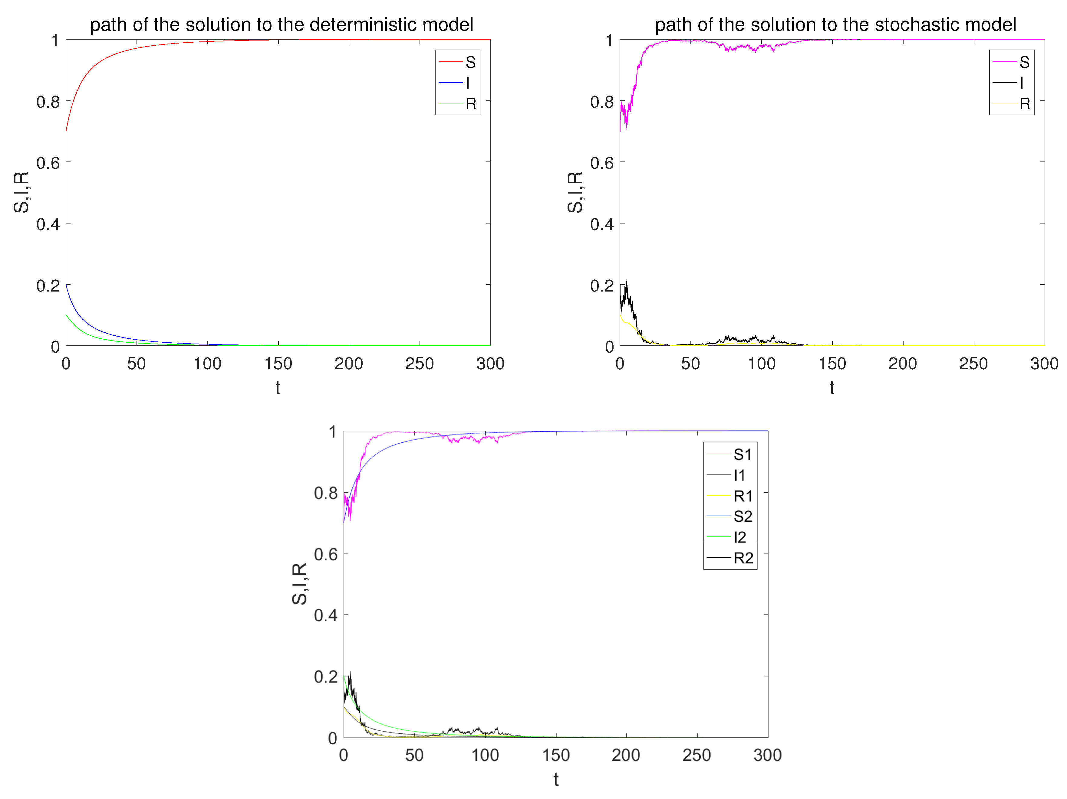
3. Extinction of the Disease

In this section, we consider the extinction of the disease of the system (4) under some sufficient assumptions.

Theorem 2.

Assume that

$${\mathcal{R}}_0<1,$$

(5)

$${\beta }_1>p{\sigma }_1^2,{\beta }_2>(1-p){\sigma }_2^2,$$

(6)

where ${\mathcal{R}}_0=\frac{{\beta }_{1}p+{\beta }_2(1-p)}{\mu +\eta +\frac{1}{2}{\sigma }_1^2{p}^2+\frac{1}{2}{\sigma }_2^2{(1-p)}^2-\frac{{\gamma }_1\eta }{\mu +{\gamma }_1+{\gamma }_2}}$, then for any initial value $\left(I\right(0),R(0\left)\right)$ in ${\mathsf{\Gamma }}_2$, the solution $\left(I\right(t),R(t\left)\right)$ of system (4) converges to $(0,0)$ a.s.

Proof. 

Let ${\mathcal{R}}_0<1$ and $\theta >1$, such that

$$-k_{\theta }\triangleq p{\beta }_1+(1-p){\beta }_2-\left(\mu +\eta +\frac{1}{2}{\sigma }_1^2{p}^2+\frac{1}{2}{\sigma }_2^2{(1-p)}^2\right)+\frac{\theta {\gamma }_1\eta }{\mu +{\gamma }_1+{\gamma }_2}<0.$$

Define the stop-time

$${\tau }_1=inf\left\{t\ge 0,I\left(t\right)\le \frac{1}{\theta }\right\}.$$

We suppose that $\mathbb{E}\left({\tau }_1\right)<\infty$. Actually, we assume that $I\left(0\right)\in (\frac{1}{\theta },1)$ (if not ${\tau }_1=0$). Hence, for all $T>0$ and $t\le T\wedge {\tau }_1$, one has

$$I\left(t\right)\ge \frac{1}{\theta }.$$

(7)

Now, employing Itô’s formula to $logI$, we have

$$\begin{array}{ll}\hfill dlogI=& \left[p{\beta }_1(1-I-R)+(1-p)\frac{{\beta }_2(1-I-R)}{1+m(1-I-R)+nI}-(\mu +\eta )+{\gamma }_1\frac{R}{I}\right.\hfill \\ \hfill & \left.-\frac{1}{2}{p}^2{\sigma }_1^2{(1-I-R)}^2-\frac{1}{2}{(1-p)}^2{\sigma }_2^2{\left(\frac{1-I-R}{1+m(1-I-R)+nI}\right)}^2\right]dt\hfill \\ \hfill & +p{\sigma }_1(1-I-R)d{B}_1\left(t\right)+(1-p)\frac{{\sigma }_2(1-I-R)}{1+m(1-I-R)+nI}d{B}_2\left(t\right)\hfill \\ \hfill \le & \left[-(\mu +\eta )+{\beta }_{1}p-\frac{1}{2}{p}^2{\sigma }_1^2+{\beta }_2(1-p)-\frac{1}{2}{(1-p)}^2{\sigma }_2^2+\theta {\gamma }_{1}R\right]dt\hfill \\ \hfill & +p{\sigma }_1(1-I-R)d{B}_1\left(t\right)+(1-p)\frac{{\sigma }_2(1-I-R)}{1+m(1-I-R)+nI}d{B}_2\left(t\right),\hfill \end{array}$$

(8)

where (6) and the monotony of the functions $x_1\mapsto -\left(\mu +{\gamma }_1+{\gamma }_2\right)+p{\beta }_1{x}_1-\frac{1}{2}{p}^2{\sigma }_1^2{x}_1^2,x_2\mapsto -\left(\mu +{\gamma }_1+{\gamma }_2\right)+(1-p)\frac{{\beta }_2{x}_2}{1+m{x}_2+nI}-\frac{1}{2}{(1-p)}^2{\sigma }_2^2{\left(\frac{x_2}{1+m{x}_2+nI}\right)}^2$ are used. Precisely, according to assumption (6), the functions $x_1$ and $x_2$ are both increasing on the interval $[0,1]$. Combining (8) and the R-equation, one has

$$\begin{array}{ll}\hfill d\left[logI+\frac{\theta {\gamma }_1}{\mu +{\gamma }_1+{\gamma }_2}R\right]\le & \left[-(\mu +\eta )+{\beta }_{1}p-\frac{1}{2}{p}^2{\sigma }_1^2+{\beta }_2(1-p)-\frac{1}{2}{(1-p)}^2{\sigma }_2^2+\frac{\theta {\gamma }_1\eta }{\mu +{\gamma }_1+{\gamma }_2}I\right]dt\hfill \\ & +p{\sigma }_1(1-I-R)d{B}_1\left(t\right)+(1-p)\frac{{\sigma }_2(1-I-R)}{1+m(1-I-R)+nI}d{B}_2\left(t\right)\hfill \\ \hfill \le & -k_{\theta }dt+p{\sigma }_1(1-I-R)d{B}_1\left(t\right)+(1-p)\frac{{\sigma }_2(1-I-R)}{1+m(1-I-R)+nI}d{B}_2\left(t\right).\hfill \end{array}$$

Further,

$$\mathbb{E}\left[logI(T\wedge {\tau }_1)+\frac{\theta {\gamma }_1}{\mu +{\gamma }_1+{\gamma }_2}R(T\wedge {\tau }_1)\right]\le logI\left(0\right)+\frac{\theta {\gamma }_1}{\mu +{\gamma }_1+{\gamma }_2}R\left(0\right)-k_{\theta }\mathbb{E}\left(T\wedge {\tau }_1\right),$$

which leads to

$$\mathbb{E}\left(T\wedge {\tau }_1\right)\le \frac{\theta {\gamma }_1}{\left(\mu +{\gamma }_1+{\gamma }_2\right)k_{\theta }}-\frac{\mathbb{E}\left[logI\left(T\wedge {\tau }_1\right)\right]}{k_{\theta }}.$$

Then, letting $T\to \infty$ and using Fatou’s lemma, we have

$$\mathbb{E}\left({\tau }_1\right)\le \frac{\theta {\gamma }_1}{\left(\mu +{\gamma }_1+{\gamma }_2\right)k_{\theta }}+\frac{log\theta }{k_{\theta }}<\infty .$$

Therefore, our claim is true. In the next step, we shall show that $I\left(t\right)$ goes by $\frac{1}{{\theta }^2}$ in a finite mean time. Therefore, we set

$$\begin{array}{c}{\tau }_1^{\prime }=inf\left\{t\ge {\tau }_1,I\left(t\right)>\frac{1}{\theta }\right\},\hfill \\ {\tau }_2=inf\left\{t<{\tau }_1^{\prime },I\left(t\right)<\frac{1}{{\theta }^2}\right\}.\hfill \end{array}$$

Hence, for all $T>0$ and any $t\in [{\tau }_1,T\wedge {\tau }_2]$ we obtain

$$\frac{1}{{\theta }^2}\le I\left(t\right)\le \frac{1}{\theta }.$$

(9)

By using (9), we can also have

$$\begin{array}{ll}\hfill d\left[logI+\frac{{\theta }^2{\gamma }_1}{\mu +{\gamma }_1+{\gamma }_2}R\right]=& \left[{\beta }_{1}p+{\beta }_2(1-p)-\left(\mu +\eta +\frac{1}{2}{p}^2{\sigma }_1^2+\frac{1}{2}{(1-p)}^2{\sigma }_2^2\right)+\frac{{\theta }^2{\gamma }_1\eta }{\mu +{\gamma }_1+{\gamma }_2}I\right]dt\hfill \\ & +p{\sigma }_1(1-I-R)d{B}_1\left(t\right)+(1-p)\frac{{\sigma }_2(1-I-R)}{1+m(1-I-R)+nI}d{B}_2\left(t\right)\hfill \\ \hfill \le & -k_{\theta }dt+p{\sigma }_1(1-I-R)d{B}_1\left(t\right)+(1-p)\frac{{\sigma }_2(1-I-R)}{1+m(1-I-R)+nI}d{B}_2\left(t\right).\hfill \end{array}$$

Integrating over $[{\tau }_1,T\wedge {\tau }_2]$, one can find

$$\mathbb{E}\left[logI\left(T\wedge {\tau }_2\right)\right]\le logI\left({\tau }_1\right)+\frac{{\theta }^2{\gamma }_1}{\mu +{\gamma }_1+{\gamma }_2}R\left({\tau }_1\right)-k_{\theta }\mathbb{E}\left(T\wedge {\tau }_2-{\tau }_1\right).$$

Thus we have

$$\mathbb{E}\left({\tau }_2\right)\le \mathbb{E}\left({\tau }_1\right)+\frac{{\theta }^2{\gamma }_1}{\left(\mu +{\gamma }_1+{\gamma }_2\right)k_{\theta }}+\frac{2log\theta }{k_{\theta }}<\infty .$$

By induction, we have the following definitions

$$\begin{array}{c}{\tau }_n^{\prime }=inf\left\{t\ge {\tau }_{n-1},I\left(t\right)>\frac{1}{{\theta }^{n-1}}\right\},\hfill \\ {\tau }_n=inf\left\{t<{\tau }_n^{\prime },I\left(t\right)<\frac{1}{{\theta }^n}\right\}.\hfill \end{array}$$

We obtain

$$\mathbb{E}\left({\tau }_n\right)\le \mathbb{E}\left({\tau }_{n-1}\right)+\frac{{\theta }^n{\gamma }_1}{\left(\mu +{\gamma }_1+{\gamma }_2\right)k_{\theta }}+\frac{nlog\theta }{k_{\theta }}<\infty .$$

(10)

Clearly, (${\tau }_n$) is an increasing sequence. Therefore, ${\tau }_n\to {\tau }_{\infty }$ a.s. We denote ${\mathsf{\Omega }}^{\prime }={\bigcap }_{n=1}^{\infty }\left({\tau }_n<\infty \right)$, by (10) and we obtain

$$\mathbb{P}\left({\mathsf{\Omega }}^{\prime }\right)=\mathbb{P}\left(\bigcap _{n=1}^{\infty }\left({\tau }_n<\infty \right)\right)=\underset{n\to \infty }{lim}\mathbb{P}\left({\tau }_n<\infty \right)=1.$$

(11)

We write ${\mathsf{\Omega }}^{\prime }$ in the following form

$${\mathsf{\Omega }}^{\prime }=\left(\left({\tau }_{\infty }<\infty \right)\cap {\mathsf{\Omega }}^{\prime }\right)\cup \left(\left({\tau }_{\infty }=\infty \right)\cap {\mathsf{\Omega }}^{\prime }\right)=\left({\tau }_{\infty }<\infty \right)\cup \left(\left({\tau }_{\infty }=\infty \right)\cap {\mathsf{\Omega }}^{\prime }\right).$$

We show that $\mathbb{P}({\tau }_{\infty }<\infty )=0$. We assume that $\mathbb{P}({\tau }_{\infty }<\infty )>0$. Let $\omega \in ({\tau }_{\infty }<\infty )$. We obtain for all $n\in {\mathbb{N}}^{*}$

$$I\left({\tau }_n\left(\omega \right)\right)=\frac{1}{a^n}.$$

By extending n to ∞, we obtain $I\left({\tau }_{\infty }\left(\omega \right)\right)=0$. Hence, ${\tau }_0\left(\omega \right)\le {\tau }_{\infty }\left(\omega \right)<\infty$, where ${\tau }_0=inf\left\{t>0,I\left(t\right)=0\right\}$. Then

$$\mathbb{P}({\tau }_0<\infty )\ge \mathbb{P}({\tau }_{\infty }<\infty )>0,$$

which is a contradiction with $\mathbb{P}({\tau }_0=\infty )=1$. Then, $\mathbb{P}({\tau }_{\infty }<\infty )=0$, furthermore

$$\mathbb{P}(({\tau }_{\infty }=\infty )\cap {\mathsf{\Omega }}^{\prime })=1.$$

Finally, we set $\omega \in ({\tau }_{\infty }=\infty )\cap {\mathsf{\Omega }}^{\prime }$, $ϵ>0$, $t>0$ and $n_0=[-logϵ{(log\theta )}^{-1}]$. For $t>{\tau }_{n_0}$, there is n such that $n\ge n_0$ and ${\tau }_n\le t\le {\tau }_{n+1}.$ Then

$$\frac{1}{{\theta }^{n+1}}\le I\left(t\right)\le \frac{1}{{\theta }^n}\le \frac{1}{{\theta }^{n_0+1}}\le ϵ,$$

which suggests

$$\underset{t\to \infty }{lim}I\left(t\right)=0.$$

(12)

This indicates that $I\left(t\right)$ converges to 0 with probability 1. Using Fatou’s lemma and the last equation of system (4), we obtain

$$\underset{t\to \infty }{lim\; sup}R\left(t\right)\le \eta {\int }_0^{\infty }\underset{t\to \infty }{lim\; sup}{e}^{-\left(\mu +{\gamma }_1+{\gamma }_2\right)u}I(t-u)du\le \frac{\eta }{\mu +{\gamma }_1+{\gamma }_2}\underset{t\to \infty }{lim\; sup}I\left(t\right),$$

which implies with (12) that ${lim}_{t\to \infty }R\left(t\right)=0.$ a.s. This proof is therefore complete.  □

4. Persistence in the Mean

Theorem 3.

Let $(S\left(0\right),I\left(0\right),R\left(0\right))\in {\mathsf{\Gamma }}_1)$ be an initial value. Assume that

$${\mathcal{R}}_s^0>1$$

holds, where ${\mathcal{R}}_s^0=\frac{p{\beta }_1+\frac{(1-p){\beta }_2}{1+m+n}}{\mu +\eta -\frac{{\gamma }_1\eta }{\mu +{\gamma }_1+{\gamma }_2}+\frac{1}{2}{p}^2{\sigma }_1^2+\frac{1}{2}{(1-p)}^2{\sigma }_2^2}$. Then, the epidemic of (3) is permanent in the mean. Precisely, we obtain

$$\underset{t\to \infty }{lim\; inf}\frac{1}{t}{\int }_0^{t}S\left(u\right)du\ge \frac{\mu }{\mu +p{\beta }_1+(1-p){\beta }_{2}C}a.s.,$$

$$\underset{t\to \infty }{lim\; inf}\frac{1}{t}{\int }_0^{t}I\left(u\right)du\ge \frac{\mu }{p{\beta }_1+\frac{(1-p){\beta }_2}{1+m+n}}\left(1-\frac{1}{{\mathcal{R}}_s^0}\right)a.s.,$$

$$\underset{t\to \infty }{lim\; inf}\frac{1}{t}{\int }_0^{t}R\left(u\right)du\ge \frac{\mu \eta }{\left(\mu +{\gamma }_1+{\gamma }_2\right)\left(p{\beta }_1+\frac{(1-p){\beta }_2}{1+m+n}\right)}\left(1-\frac{1}{{\mathcal{R}}_s^0}\right)a.s.$$

Proof. 

Integrating the first equation of (3) between 0 and t, we obtain

$$\begin{array}{ll}\hfill \mu t-\left(S\right(t)-S(0\left)\right)=& {\int }_0^t\left(\mu S+p{\beta }_{1}SI+\frac{(1-p){\beta }_{2}SI}{1+mS+nI}-{\gamma }_{2}R\right)ds\hfill \\ & +{\int }_0^{t}p{\sigma }_{1}SId{B}_1\left(s\right)+{\int }_0^t\frac{(1-p){\sigma }_{2}SI}{1+mS+nI}d{B}_2\left(s\right)\hfill \\ \hfill \le & {\int }_0^t\left(\mu +p{\beta }_{1}I+\frac{(1-p){\beta }_{2}I}{1+mS+nI}\right)Sds\hfill \\ & +{\int }_0^{t}p{\sigma }_{1}SId{B}_1\left(s\right)+{\int }_0^t\frac{(1-p){\sigma }_{2}SI}{1+mS+nI}d{B}_2\left(s\right).\hfill \end{array}$$

It is obvious that $p{\beta }_{1}SI<p{\beta }_1$, $\frac{SI}{1+mS+nI}<C$, where C is a positive constant. Thus, we have

$$\begin{array}{ll}\hfill \mu t-\left(S\right(t)-S(0\left)\right)\le & \left(\mu +p{\beta }_1+(1-p){\beta }_{2}C\right){\int }_0^{t}Sds\hfill \\ & +{\int }_0^{t}p{\sigma }_{1}SId{B}_1\left(s\right)+{\int }_0^t\frac{(1-p){\sigma }_{2}SI}{1+mS+nI}d{B}_2\left(s\right).\hfill \end{array}$$

Multiplying both sides by $\frac{1}{t}$, we obtain

$$\begin{array}{ll}\hfill \frac{1}{t}{\int }_0^{t}Sds\ge & \frac{1}{\mu +p{\beta }_1+(1-p){\beta }_{2}C}\left(\mu -\frac{S\left(t\right)-S\left(0\right)}{t}\right)\hfill \\ & -\frac{1}{\mu +p{\beta }_1+(1-p){\beta }_{2}C}\left(\frac{1}{t}{\int }_0^{t}p{\sigma }_{1}SId{B}_1\left(s\right)+\frac{1}{t}{\int }_0^t\frac{(1-p){\sigma }_{2}SI}{1+mS+nI}d{B}_2\left(s\right)\right).\hfill \end{array}$$

Note that ${\int }_0^{t}p{\sigma }_{1}SId{B}_1\left(s\right)$, ${\int }_0^t\frac{(1-p){\sigma }_{2}SI}{1+mS+nI}d{B}_2\left(s\right)$ are continuous martingales with finite quadratic variation. By employing the strong law of large numbers for local martingales, we have

$$\underset{t\to \infty }{lim}\frac{S\left(t\right)-S\left(0\right)}{t}+\frac{1}{t}{\int }_0^{t}p{\sigma }_{1}SId{B}_1\left(s\right)+\frac{1}{t}{\int }_0^t(1-p)\frac{{\sigma }_{2}SI}{1+mS+nI}d{B}_2\left(s\right)=0a.s.$$

Hence,

$$\underset{t\to \infty }{lim}\frac{1}{t}{\int }_0^{t}Sds\ge \frac{\mu }{\mu +p{\beta }_1+(1-p){\beta }_{2}C}a.s.$$

Then, we define a function F on ${\mathsf{\Gamma }}_1$

$$F(S,I,R)=logI+\frac{p{\beta }_1+\frac{(1-p){\beta }_2}{1+m+n}}{\mu }S+BlogR,$$

(13)

where B is the unique solution to the equation

$$-\left(\mu +{\gamma }_1+{\gamma }_2\right)B+2\sqrt{{\gamma }_1\eta }\sqrt{B}-\frac{{\gamma }_1\eta }{\mu +{\gamma }_1+{\gamma }_2}=0,$$

(14)

given by $B=\frac{{\gamma }_1\eta }{{\left(\mu +{\gamma }_1+{\gamma }_2\right)}^2}$. Using ${(1-I-R)}^2\le 1$ and (8) we infer that

$$\begin{array}{ll}\hfill dlogI\ge & \left[p{\beta }_{1}S+(1-p)\frac{{\beta }_{2}S}{1+mS+nI}-\left(\mu +\eta +\frac{1}{2}{p}^2{\sigma }_1^2+\frac{1}{2}{(1-p)}^2{\sigma }_2^2\right)+{\gamma }_1\frac{R}{I}\right]dt\hfill \\ & +p{\sigma }_{1}Sd{B}_1\left(t\right)+\frac{(1-p){\sigma }_{2}S}{1+mS+nI}d{B}_2\left(t\right).\hfill \end{array}$$

(15)

Additionally, we also have

$$\begin{array}{rr}\hfill d\left(\frac{p{\beta }_1+\frac{(1-p){\beta }_2}{1+m+n}}{\mu }S\right)=& [p{\beta }_1+\frac{(1-p){\beta }_2}{1+m+n}-p{\beta }_{1}S-\frac{(1-p){\beta }_{2}S}{1+m+n}-\frac{p^2{\beta }_1^{2}SI}{\mu }-\frac{p(1-p){\beta }_1{\beta }_{2}SI\frac{SI}{1+m+n}}{\mu }\hfill \\ & -\frac{p(1-p){\beta }_1{\beta }_{2}SI\frac{SI}{1+mS+nI}}{\mu }-\frac{\frac{{\beta }_2^2{(1-p)}^{2}SI}{(1+m+n)(1+mS+nI)}}{\mu }+\frac{{\gamma }_2(p{\beta }_1+\frac{(1-p){\beta }_2}{1+m+n})R}{\mu }]dt\hfill \\ & -\frac{p{\beta }_1+\frac{(1-p){\beta }_2}{1+m+n}}{\mu }p{\sigma }_{1}SId{B}_1\left(t\right)-\frac{p{\beta }_1+\frac{(1-p){\beta }_2}{1+m+n}}{\mu }\frac{(1-p){\sigma }_{2}SI}{1+mS+nI}d{B}_2\left(t\right)\hfill \\ \hfill \ge & \left[p{\beta }_1+\frac{(1-p){\beta }_2}{1+m+n}-p{\beta }_{1}S-\frac{(1-p){\beta }_{2}S}{1+m+n}-\frac{{(p{\beta }_1+(1-p){\beta }_2)}^2}{\mu }I\right]dt\hfill \\ & -\frac{p{\beta }_1+\frac{(1-p){\beta }_2}{1+m+n}}{\mu }p{\sigma }_{1}SId{B}_1\left(t\right)-\frac{p{\beta }_1+\frac{(1-p){\beta }_2}{1+m+n}}{\mu }\frac{(1-p){\sigma }_{2}SI}{1+mS+nI}d{B}_2\left(t\right).\hfill \end{array}$$

(16)

Moreover,

$$dBlogR=\left[\eta B\frac{I}{R}-(\mu +{\gamma }_1+{\gamma }_2)B\right]dt.$$

(17)

Combining (15)–(17), we have

$$\begin{array}{ll}\hfill dF(S,I,R)\ge & \left[p{\beta }_1+\frac{(1-p){\beta }_2}{1+m+n}-\left(\mu +\eta +\frac{1}{2}{p}^2{\sigma }_1^2+\frac{1}{2}{(1-p)}^2{\sigma }_2^2\right)-\left(\mu +{\gamma }_1+{\gamma }_2\right)B\right.\hfill \\ & +{(\sqrt{\frac{{\gamma }_{1}R}{I}}-\sqrt{\frac{B\eta I}{R}})}^2\left.+2\sqrt{{\gamma }_1\eta B}-\frac{{\left(p{\beta }_1+(1-p){\beta }_2\right)}^2}{\mu }I\right]dt\hfill \\ & +\left(1-\frac{p{\beta }_1+\frac{(1-p){\beta }_2}{1+m+n}}{\mu }I\right)p{\sigma }_{1}Sd{B}_1\left(t\right)+\left(1-\frac{p{\beta }_1+\frac{(1-p){\beta }_2}{1+m+n}}{\mu }I\right)\frac{(1-p){\sigma }_{2}S}{1+mS+nI}d{B}_2\left(t\right)\hfill \\ \hfill \ge & \left[p{\beta }_1+\frac{(1-p){\beta }_2}{1+m+n}-\left(\mu +\eta +\frac{1}{2}{p}^2{\sigma }_1^2+\frac{1}{2}{(1-p)}^2{\sigma }_2^2\right)-\left(\mu +{\gamma }_1+{\gamma }_2\right)B\right.\hfill \\ & \left.+2\sqrt{{\gamma }_1\eta B}-\frac{{\left(p{\beta }_1+(1-p){\beta }_2\right)}^2}{\mu }I\right]dt\hfill \\ & +\left(1-\frac{p{\beta }_1+\frac{(1-p){\beta }_2}{1+m+n}}{\mu }I\right)p{\sigma }_{1}Sd{B}_1\left(t\right)+\left(1-\frac{p{\beta }_1+\frac{(1-p){\beta }_2}{1+m+n}}{\mu }I\right)\frac{(1-p){\sigma }_{2}S}{1+mS+nI}d{B}_2\left(t\right).\hfill \end{array}$$

By using (14), we have

$$\begin{array}{ll}\hfill dF(S,I,R)\ge & \left[\left(p{\beta }_1+\frac{(1-p){\beta }_2}{1+m+n}\right)\left(1-\frac{1}{{\mathcal{R}}_s^0}\right)\left.-\frac{{\left(p{\beta }_1+(1-p){\beta }_2\right)}^2}{\mu }I\right]dt\right.\hfill \\ & +\left(1-\frac{p{\beta }_1+\frac{(1-p){\beta }_2}{1+m+n}}{\mu }I\right)p{\sigma }_{1}Sd{B}_1\left(t\right)+\left(1-\frac{p{\beta }_1+\frac{(1-p){\beta }_2}{1+m+n}}{\mu }I\right)\frac{(1-p){\sigma }_{2}S}{1+mS+nI}d{B}_2\left(t\right).\hfill \end{array}$$

(18)

Integrating the last inequality from 0 to t and multiplying by $\frac{1}{t}$, it yields that

$$\begin{array}{ll}\hfill \frac{F\left(S\right(t),I(t),R(t\left)\right)-F\left(S\right(0),I(0),R(0\left)\right)}{t}\ge & \left(p{\beta }_1+\frac{(1-p){\beta }_2}{1+m+n}\right)\left(1-\frac{1}{{\mathcal{R}}_s^0}\right)\hfill \\ & -\frac{{(p{\beta }_1+(1-p){\beta }_2)}^2}{\mu t}{\int }_0^{t}I\left(u\right)du+\frac{M_1\left(t\right)}{t}+\frac{M_2\left(t\right)}{t},\hfill \end{array}$$

where

$$M_1\left(t\right)=p{\sigma }_1{\int }_0^{t}S\left(u\right)\left(1-\frac{p{\beta }_1+\frac{(1-p){\beta }_2}{1+m+n}}{\mu }I\left(u\right)\right)d{B}_1\left(u\right),$$

and

$$M_2\left(t\right)=(1-p){\sigma }_2{\int }_0^t\frac{{\sigma }_{2}S\left(u\right)}{1+mS\left(u\right)+nI\left(u\right)}\left(1-\frac{p{\beta }_1+\frac{(1-p){\beta }_2}{1+m+n}}{\mu }I\left(u\right)\right)d{B}_2\left(u\right).$$

Therefore

$$\begin{array}{ll}\hfill \frac{1}{t}{\int }_0^{t}I\left(u\right)du\ge & \frac{\mu (p{\beta }_1+\frac{(1-p){\beta }_2}{1+m+n})}{{(p{\beta }_1+(1-p){\beta }_2)}^2}\left(1-\frac{1}{{\mathcal{R}}_s^0}\right)-\frac{\mu }{{(p{\beta }_1+(1-p){\beta }_2)}^2}\frac{F\left(S\right(t),I(t),R(t\left)\right)}{t}\hfill \\ & +\frac{\mu }{{(p{\beta }_1+(1-p){\beta }_2)}^2}\frac{F\left(S\right(0),I(0),R(0\left)\right)}{t}\hfill \\ & +\frac{\mu }{{(p{\beta }_1+(1-p){\beta }_2)}^2}\frac{M_{1}t}{t}+\frac{\mu }{{(p{\beta }_1+(1-p){\beta }_2)}^2}\frac{M_{2}t}{t}.\hfill \end{array}$$

Clearly, $M_1\left(t\right)$,$M_2\left(t\right)$ are continuous martingales and $M_1\left(0\right)=0$, $M_2\left(0\right)=0$ with their quadratic variation

$$\left[M_1\right]\left(t\right)=p^2{{\sigma }_1}^2{\int }_0^t{\left[S^2\left(u\right)\left(1-\frac{p{\beta }_1+\frac{(1-p){\beta }_2}{1+m+n}}{\mu }I\left(u\right)\right)\right]}^{2}du<p^2{{\sigma }_1}^2(1+\frac{p{\beta }_1+\frac{(1-p){\beta }_2}{1+m+n}}{\mu }{)}^{2}t,$$

$$\begin{array}{ll}\hfill \left[M_2\right]\left(t\right)=& {(1-p)}^2{{\sigma }_2}^2{\int }_0^t(1-\frac{p{\beta }_1+\frac{(1-p){\beta }_2}{1+m+n}}{\mu }I\left(u\right){)}^2{\left(\frac{S\left(u\right)}{1+mS\left(u\right)+nI\left(u\right)}\right)}^{2}du\hfill \\ \hfill <& {(1-p)}^2{{\sigma }_2}^2(1+\frac{p{\beta }_1+\frac{(1-p){\beta }_2}{1+m+n}}{\mu }{)}^{2}t.\hfill \end{array}$$

Hence, by the strong law of large numbers for local martingales, we have

$$\underset{t\to \infty }{lim}\frac{1}{t}\frac{M_1\left(t\right)}{t}=0a.s.,$$

$$\underset{t\to \infty }{lim}\frac{1}{t}\frac{M_2\left(t\right)}{t}=0a.s.$$

Consequently, we have

$$\underset{t\to \infty }{lim}inf\frac{1}{t}{\int }_0^{t}I\left(u\right)du\ge \frac{\mu \left(p{\beta }_1+\frac{(1-p){\beta }_2}{1+m+n}\right)}{{(p{\beta }_1+(1-p){\beta }_2)}^2}\left(1-\frac{1}{{\mathcal{R}}_s^0}\right)-\frac{\mu }{{(p{\beta }_1+(1-p){\beta }_2)}^2}\underset{t\to \infty }{lim}sup\frac{F\left(S\right(t),I(t),R(t\left)\right)}{t}a.s.$$

(19)

Clearly,

$$\underset{t\to \infty }{lim}sup\frac{F\left(S\right(t),I(t),R(t\left)\right)}{t}\le \underset{t\to \infty }{lim}sup\frac{p{\beta }_1+\frac{(1-p){\beta }_2}{1+m+n}}{\mu t}=0.$$

Combining (19), we find the desired result.

$$\underset{t\to \infty }{lim}inf\frac{1}{t}{\int }_0^{t}I\left(u\right)du\ge \frac{\mu \left[p{\beta }_1+\frac{(1-p){\beta }_2}{1+m+n}\right]}{{(p{\beta }_1+(1-p){\beta }_2)}^2}\left(1-\frac{1}{{\mathcal{R}}_s^0}\right)a.s.$$

(20)

Integrating the last equation of (3) and multiplying by $\frac{1}{t}$, we obtain

$$\frac{\mu +{\gamma }_1+{\gamma }_2}{t}{\int }_0^{t}R\left(s\right)ds=\frac{\eta }{t}{\int }_0^{t}I\left(s\right)ds+\frac{R\left(0\right)-R\left(t\right)}{t}.$$

As $\underset{t\to \infty }{lim}\frac{R\left(0\right)-R\left(t\right)}{t}=0$, using (20), we deduce that

$$\underset{t\to \infty }{lim}inf\frac{1}{t}{\int }_0^{t}R\left(s\right)ds\ge \frac{\eta \mu \left(p{\beta }_1+\frac{(1-p){\beta }_2}{1+m+n}\right)}{(\mu +{\gamma }_1+{\gamma }_2){(p{\beta }_1+(1-p){\beta }_2)}^2}\left(1-\frac{1}{{\mathcal{R}}_s^0}\right).$$

Hence, we complete the proof. □

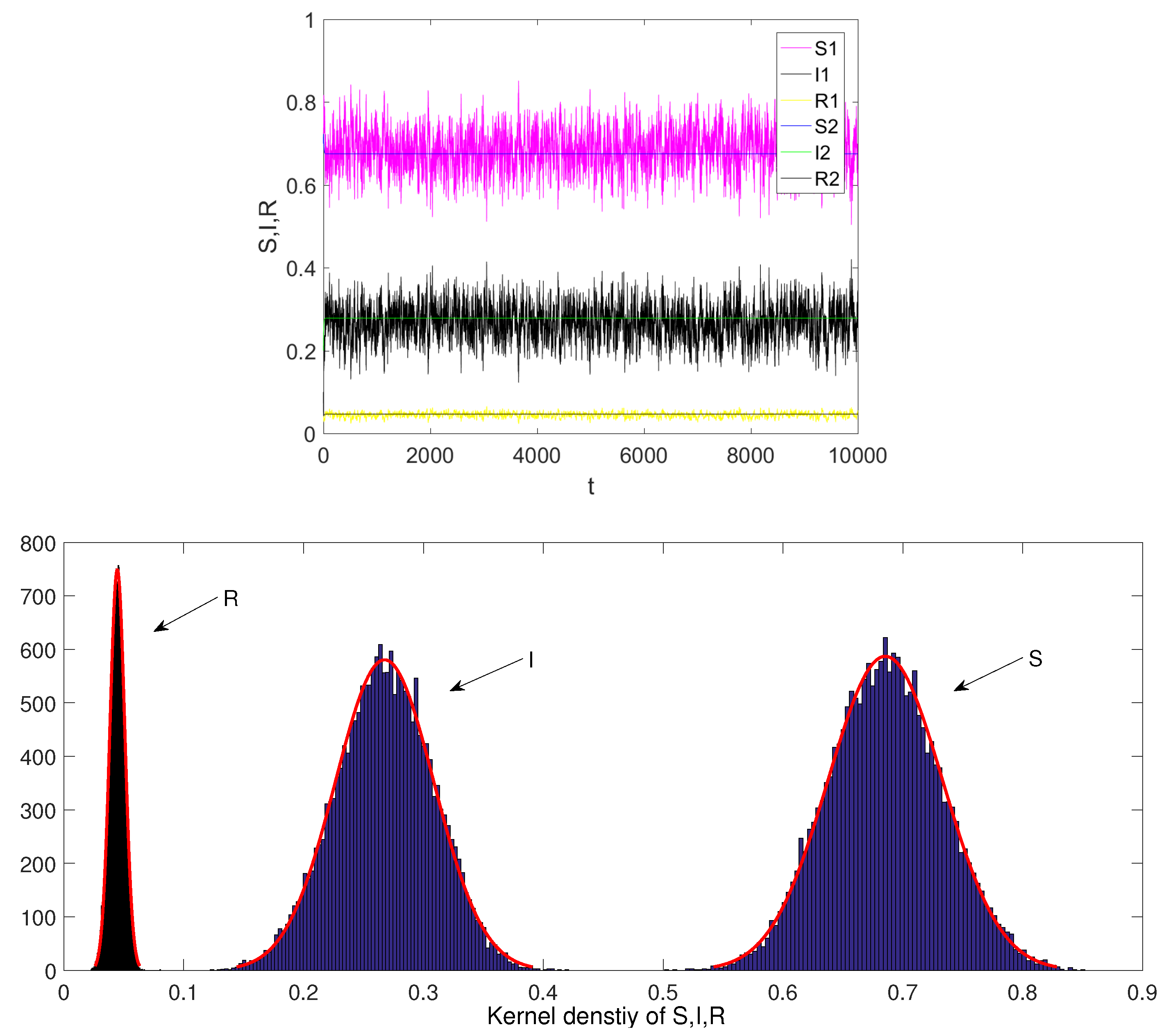
5. Existence of a Stationary Distribution

In Section 4, we obtain that the persistence in the mean of the system starts from any initial condition of the invariant region ${\mathsf{\Gamma }}_1$ on certain conditions. In this section, to better understand the asymptotic behavior of the diseases shown in the SDE system (4), in the case of ${\mathcal{R}}_s^0>1$, we present that there exists a stationary distribution of the process $\left(I\right(t),R(t\left)\right)$. The diffusion matrix of system (4) is shown as

$$\sum (i,r)=\left(\begin{array}{c}{\left(p{\sigma }_1(1-i-r)i+(1-p)\frac{{\sigma }_2(1-i-r)i}{1+m(1-i-r)+ni}\right)}^2\\ 0\end{array}\right.\left.\begin{array}{c}0\hfill \\ 0\hfill \end{array}\right).$$

As the diffusion matrix is degenerate and dissatisfies the uniform ellipticity condition, we can not directly prove the asymptotic stability using Khasminskii’s theorem [23]. To handle this situation, we apply the integral Markov semigroup theory, presented in [14,24,25].

Now, we consider the space $({\mathsf{\Gamma }}_2,\mathcal{B}\left({\mathsf{\Gamma }}_2\right),m)$, where $\mathcal{B}\left({\mathsf{\Gamma }}_2\right)$ is the $\sigma$-algebra of Borel subsets of ${\mathsf{\Gamma }}_2$ and m is the Lebesgue measure on $({\mathsf{\Gamma }}_2,\mathcal{B}\left({\mathsf{\Gamma }}_2\right))$. Throughout this section, we denote the transition probability function for the diffusion process $\left(I\right(t),R(t\left)\right)$, i.e.,

$$P(t,i_0,r_0,B)=\mathbb{P}((I\left(t\right),R\left(t\right))\in B|I\left(0\right)=i_0,R\left(0\right)=r_0).$$

In Theorem 4, we show the absolute continuity of the transition function of the degenerate diffusion processes, as described by the Stratonovich equation, using the Hörmander condition, given in [26]. Let $\mathcal{K}(t,i,r,i_0,r_0)$ be the density of $P(t,i_0,r_0,.)$. For any $t\ge 0$, the operator $P\left(t\right)$ can be defined as follows

$$P\left(t\right)g(i,r)={\int }_{{\mathsf{\Gamma }}_2}\mathcal{K}(t,i,r,i_0,r_0)g(i,r)m(di,dr),g\in \mathcal{D}.$$

Hence, according to system (4), we define the integral Markov semigroup ${\left\{P\left(t\right)\right\}}_{t\ge 0}$.

Theorem 4.

The transition probability function $P(t,i_0,r_0,.)$ of the solution $\left(I\right(t),R(t\left)\right)$ of system (4), has a density $\mathcal{K}(t,i,r,i_0,r_0)\in {\mathcal{C}}^{\infty }(\mathbb{R},{\mathsf{\Gamma }}_2,{\mathsf{\Gamma }}_2)$.

Proof. 

Denote $a\left(x\right)$ and $b\left(x\right)$ two vectors fields defined on ${\mathbb{R}}^n$, then the Lie bracket $[a,b]\left(x\right)$ is presented as

$${[a,b]}_j\left(x\right)=\sum _{k=1}^n[a_k\frac{\partial b_j}{\partial x_k}\left(x\right)-b_k\frac{\partial a_j}{\partial x_k}\left(x\right)],$$

$j=1,\dots ,n.$ We write the Itô system (4) as the Stratonovitch SDE

$$\left(\begin{array}{c}dI\hfill \\ dR\hfill \end{array}\right)=\left(\begin{array}{c}{a}_1(I,R)\hfill \\ a_2(I,R)\hfill \end{array}\right)dt+\left(\begin{array}{c}p{\sigma }_1(1-I-R)I+(1-p)\frac{{\sigma }_2(1-I-R)I}{1+m(1-I-R)+nI}\\ 0\end{array}\right)\circ dB\left(t\right),$$

(21)

where

$$\begin{array}{c}{a}_1(I,R)=p{\beta }_1(1-I-R)I+(1-p)\frac{{\beta }_2(1-I-R)I}{1+m(1-I-R)+nI}-(\mu +\eta )I+{\gamma }_{1}R,\hfill \\ a_2(I,R)=\eta I-(\mu +{\gamma }_1+{\gamma }_2)R.\hfill \end{array}$$

Let $a(I,R)={(a_1(I,R),a_2(I,R))}^{\prime }$ and $b(I,R)={(p{\sigma }_1(1-I-R)I+(1-p)\frac{{\sigma }_2(1-I-R)I}{1+m(1-I-R)+nI},0)}^{\prime }$. By direct calculation, we obtain $det([a,b](I,R),b(I,R))=\eta {(p{\sigma }_1(1-I-R)I+(1-p)\frac{{\sigma }_2(1-I-R)I}{1+m(1-I-R)+nI})}^2>0$ for any $[I,R]\in {\mathsf{\Gamma }}_2$. Accordingly, the vectors $[a,b](I,R)$ and $b(I,R)$ span the space $\mathsf{\Gamma }{2}_{}$. By employing the Hörmander theorem, the probability function $P(t,i_0,r_0,.)$ has a density $\mathcal{K}(t,i,r,i_0,r_0)\in {\mathcal{C}}^{\infty }(\mathbb{R},{\mathsf{\Gamma }}_2,{\mathsf{\Gamma }}_2)$. □

Now we use the approach given in [24,25] to verify that $\mathcal{K}$ is positive. We fix a function $\varphi \in C\left(\right[0,T],R)$. Consider the system of differential equations below

$$\left\{\begin{array}{c}{\dot{I}}_{\varphi }\left(t\right)=a_1(I_{\varphi }\left(t\right),R_{\varphi }\left(t\right))+(p{\sigma }_1(1-I_{\varphi }\left(t\right)-R_{\varphi }\left(t\right))I_{\varphi }\left(t\right)+(1-p)\frac{{\sigma }_2(1-I_{\varphi }\left(t\right)-R_{\varphi }\left(t\right))I_{\varphi }\left(t\right)}{1+m(1-I_{\phi }\left(t\right)-R_{\phi }\left(t\right))+n{I}_{\phi }\left(t\right)}\phi \left(t\right),\hfill \\ {\dot{R}}_{\varphi }\left(t\right)=a_2(I_{\varphi }\left(t\right),R_{\varphi }\left(t\right)),\hfill \end{array}\right.$$

(22)

with the initial condition $I_{\varphi }\left(0\right)=i_0$, $R_{\varphi }\left(0\right)=r_0$ and let $D_{i_0,r_0,\varphi }$ be the Frechét derivative of the function $h\to \left(\begin{array}{c}{I}_{\varphi +h}\left(T\right)\hfill \\ R_{\varphi +h}\left(T\right)\hfill \end{array}\right)$ from $\mathcal{C}\left(\right[0,T],R)$ to ${\mathbb{R}}^2$. The derivative $D_{i_0,r_0,\varphi }$ could be found as follows. Let $E\left(t\right)=a^{\prime }(I_{\varphi }\left(t\right),R_{\varphi }\left(t\right))+\varphi \left(t\right)b^{\prime }(I_{\varphi }\left(t\right),R_{\varphi }\left(t\right))$, where $a^{\prime }$ and $b^{\prime }$ are the Jacobian of $a(I,R)$ and $b(I,R)$, respectively. Denote $Q(t,t_0)$, for $0\le t_0\le t\le T$, as the function satisfying $Q(t_0,t_0)=I$, $\frac{\partial Q}{\partial t}(t,t_0)=E\left(t\right)Q(t,t_0)$. Then

$$D_{i_0,r_0,\varphi }h={\int }_0^{T}Q(T,s)b(I_{\varphi }\left(s\right),R_{\varphi }\left(s\right))h\left(s\right)ds.$$

If, for some $\varphi \in \mathcal{C}\left(\right[0,T],R)$, the derivative $D_{i_0,r_0,\varphi }$ has rank 2, then $\mathcal{K}(t,i,r,i_0,r_0)>0$ for $i=I_{\varphi }\left(T\right)$ and $r=R_{\varphi }\left(T\right)$.

Theorem 5.

For each $(i_0,r_0)\in {\mathsf{\Gamma }}_2$ and $\varphi \in \mathcal{C}\left(\right[0,T],\mathbb{R})$, the derivative $D_{i_0,r_0,\varphi }$ has rank 2.

Proof. 

Let $ϵ\in (0,T)$ and $h=1_{[T-ϵ,T]}$. By a first-order Taylor series approximation, we obtain $Q(T,s)=1-E\left(T\right)(T-s)+o(T-s)$. Then $D_{i_0,r_0,\varphi }h=ϵe-\frac{1}{2}{ϵ}^{2}E\left(T\right)e+o\left({ϵ}^2\right)$ where $e=\left(\begin{array}{c}1\hfill \\ 0\hfill \end{array}\right)$. By computation we have

$$E\left(T\right)e=\left(\begin{array}{c}p({\beta }_1+\varphi {\sigma }_1){\phi }_{\varphi }\left(t\right)+(1-p)({\beta }_2+\varphi {\sigma }_2)(\frac{{\phi }_{\varphi }\left(t\right)}{1+m{\rho }_{\varphi }\left(t\right))+n{I}_{\varphi }\left(t\right)}-\frac{(n-m){\rho }_{\varphi }\left(t\right)I_{\varphi }\left(t\right)}{{(1+m{\rho }_{\varphi }\left(t\right))+n{I}_{\varphi }\left(t\right))}^2}-(\mu +\eta )\\ \eta \end{array}\right).$$

where ${\phi }_{\varphi }\left(t\right)=1-2I_{\varphi }\left(t\right)-R_{\varphi }\left(t\right)$ and ${\rho }_{\varphi }\left(t\right)=1-I_{\varphi }\left(t\right)-R_{\varphi }\left(t\right)$. Therefore, e and $E\left(t\right)e$ are linearly independent and the derivative $D_{i_0,r_0,\varphi }$ has rank 2. □

Now we verify the positivity of $\mathcal{K}$. Hence, we investigate the controllability of the region ${\mathsf{\Gamma }}_2$.

Theorem 6.

For each $(I_0,R_0)\in {\mathsf{\Gamma }}_2$ and for almost every $(I_1,R_1)\in {\mathsf{\Gamma }}_2$, there exists $T>0$, such that $\mathcal{K}(T,I_1,R_1,I_0,R_0)>0$.

Proof. 

Fixed $(i_0,r_0)$, $(i_1,r_1)\in {\mathsf{\Gamma }}_2$. Without a loss of generality, we assume that $r_1<r_0$. Now we show that there is a control function $\varphi$ and $T>0$ such that $I_{\varphi }\left(0\right)=i_0$, $R_{\varphi }\left(0\right)=r_0$, $I_{\varphi }\left(T\right)=i_1$, $R_{\varphi }\left(T\right)=r_1$. We first consider the following ODEs

$$\left\{\begin{array}{c}{\dot{X}}_1=-(\mu +{\gamma }_1+{\gamma }_2)X_1,\hfill \\ {\dot{Y}}_1=\eta -(\mu +{\gamma }_1+{\gamma }_2+\eta )Y_1,\hfill \\ X_1\left(0\right)=Y_1\left(0\right)=r_0,\hfill \end{array}\right.$$

(23)

with positive solutions $X_1$ and $Y_1$. We define the function $R_1\left(t\right)$, as follows

$$R_1\left(t\right)=X_1\left(t\right)+\frac{i_0}{1-r_0}(Y_1\left(t\right)-X_1\left(t\right)).$$

Thus, we have

$$R_1\left(0\right)=r_0,{\dot{R}}_1\left(0\right)=\eta i_0-(\mu +{\gamma }_1+{\gamma }_2).$$

(24)

Furthermore

$$\begin{array}{ll}\hfill {\dot{R}}_1\left(t\right)& =-(\mu +{\gamma }_1+{\gamma }_2)R_1\left(t\right)+\frac{\lambda i_0}{1-r_0}(1-Y_1\left(t\right)),\hfill \\ & =\eta -(\mu +{\gamma }_1+{\gamma }_2+\eta )R_1\left(t\right)+\frac{\eta (1-i_0-r_0)}{1-r_0}(X_1\left(t\right)-1).\hfill \end{array}$$

As $X_1\left(t\right),Y_1\left(t\right)\in (0,1)$ for all $t\ge 0$. Then

$$-(\mu +{\gamma }_1+{\gamma }_2)R_1\left(t\right)<{\dot{R}}_1\left(t\right)<\eta -(\mu +{\gamma }_1+{\gamma }_2+\eta )R_1\left(t\right).$$

(25)

Similarly, we consider $X_2$ and $Y_2$ the solutions of the ODEs

$$\left\{\begin{array}{c}{\dot{X}}_2=-(\mu +{\gamma }_1+{\gamma }_2)X_2,\hfill \\ {\dot{Y}}_2=\eta -(\mu +{\gamma }_1+{\gamma }_2+\eta )Y_2,\hfill \\ X_2\left(0\right)=Y_2\left(0\right)=r_1.\hfill \end{array}\right.$$

(26)

Then, the function

$$Z\left(t\right)=X_2\left(t\right)+\frac{i_1}{1-r_1}(Y_2\left(t\right)-X_2\left(t\right)),$$

verifies the following

$$Z\left(0\right)=r_1,\dot{Z}\left(0\right)=\eta i_1-(\mu +{\gamma }_1+{\gamma }_2)r_1.$$

(27)

Now, we choose a differentiable function, $R_3\left(t\right)=Z(t-T)$, where T is a sufficiently large number, such that

$$X_1\left(t\right)\le R_3\left(t\right)\le Y_1\left(t\right),\forall t\in [T-\epsilon ,\epsilon ],$$

(28)

where $\epsilon$ is a small enough positive number. Hence, from (27) and (28) we get that for all $t\in [T-\epsilon ,T]$, $R_3\left(t\right)$ verifies

$$-(\mu +{\gamma }_1+{\gamma }_2)R_3\left(t\right)<{\dot{R}}_3\left(t\right)<\eta -(\mu +{\gamma }_1+{\gamma }_2+\eta )R_3\left(t\right),$$

(29)

$$R_2\left(T\right)=r_1,{\dot{R}}_2\left(T\right)=\eta i_1-(\mu +{\gamma }_1+{\gamma }_2)r_1.$$

(30)

Finally, we define a function $R_2\left(t\right)$ on $[\epsilon ,T-\epsilon ]$ such that $X_1\left(t\right)\le R_2\left(t\right)\le Y_1\left(t\right)$, then we have

$$-(\mu +{\gamma }_1+{\gamma }_2)R_2\left(t\right)<{\dot{R}}_2\left(t\right)<\eta -(\mu +{\gamma }_1+{\gamma }_2+\eta )R_2\left(t\right).$$

(31)

In addition, we choose $R_2\left(t\right)$ appropriate to define the ${\mathcal{C}}^1$-function $R_{\varphi }$ as follows

$$R_{\varphi }\left(t\right)=\left\{\begin{array}{c}{R}_1\left(t\right),0\le t\le \epsilon ,\hfill \\ R_2\left(t\right),\epsilon \le t\le T-\epsilon ,\hfill \\ R_3\left(t\right),T-\epsilon \le t\le T.\hfill \end{array}\right.$$

Hence the function $R_{\varphi }$, constructed above, possesses the properties below

$$\begin{array}{ll}\hfill & R_{\varphi }\left(0\right)=r_0,R_{\varphi }\left(t\right)=r_1,\hfill \\ \hfill & {\dot{R}}_{\varphi }\left(0\right)=\eta i_0-(\mu +{\gamma }_1+{\gamma }_2)r_0,{\dot{R}}_{\varphi }\left(T\right)=\eta i_1-(\mu +{\gamma }_1+{\gamma }_2)r_1,\hfill \\ \hfill & -(\mu +{\gamma }_1+{\gamma }_2)R_{\varphi }\left(t\right)<{\dot{R}}_{\varphi }\left(t\right)<\eta -(\mu +{\gamma }_1+{\gamma }_2+\eta )R_{\varphi }\left(t\right).\hfill \end{array}$$

(32)

Now, we define the function $I_{\varphi }\left(t\right)$ on the interval $[0,T]$ by

$$I_{\varphi }\left(t\right)=\frac{1}{\eta }({\dot{R}}_{\varphi }\left(t\right)+(\mu +{\gamma }_1+{\gamma }_2)R_{\varphi }\left(t\right)).$$

Thus, we can deduce from (32) that $0<I_{\varphi }\left(t\right)+R_{\varphi }\left(t\right)<1$ for all $t\in [0,T]$. After that, we choose the control function $\varphi \left(t\right)$ as follows

$$\varphi \left(t\right)=\frac{{\dot{I}}_{\varphi }\left(t\right)-a_1(I_{\varphi }\left(t\right),R_{\varphi }\left(t\right))}{[(p{\sigma }_1(1-I_{\varphi }\left(t\right)-R_{\varphi }\left(t\right))+(1-p)\frac{{\sigma }_2(1-I_{\varphi }\left(t\right)-R_{\varphi }\left(t\right))}{1+m(1-I_{\varphi }\left(t\right)-R_{\varphi }\left(t\right))+n{I}_{\varphi }\left(t\right)}]I_{\varphi }\left(t\right)}.$$

Therefore, with the above determinate continuous function $\varphi$, $(I_{\varphi }\left(t\right),R_{\varphi }\left(t\right))$ is the solution to system (22). Furthermore, from (32) and the chosen of $I_{\varphi }\left(t\right)$, we find that this solution satisfies

$$(I_{\varphi }\left(0\right),R_{\varphi }\left(0\right))=(i_0,r_0),(I_{\varphi }\left(T\right),R_{\varphi }\left(T\right))=(i_1,r_1).$$

This completes the proof. □

Theorem 7.

If ${\mathcal{R}}_s^0>1$, then the semigroup ${\left\{P\left(t\right)\right\}}_{t\ge 0}$ is asymptotically stable. This indicates that there exists a unique density ${\mathcal{K}}^{*}(i,r)$, such that

$$\int {\int }_{{\mathsf{\Gamma }}_2}|\mathcal{K}(t,i,r,i_0,r_0)-{\mathcal{K}}^{*}(i,r)|didr=0forall(i_0,r_0)\in {\mathsf{\Gamma }}_2.$$

Proof. 

First, we construct a positive ${\mathcal{C}}^2$-function ${\mathbf{V}}_2$ and a closed set $\Delta \subset {\mathsf{\Gamma }}_2$ such that

$$\underset{(I,R)\in {\mathsf{\Gamma }}_2\backslash \Delta }{sup}\mathcal{L}{\mathbf{V}}_2(I,R)<0,$$

where $\mathcal{L}$ is the differential operator related to the system (4) and $\Delta =({\alpha }_1,{\alpha }_2)\times ({\alpha }_3,{\alpha }_4)\subset {\mathsf{\Gamma }}_2$ in which $\alpha$, ${\alpha }_1$, ${\alpha }_2$, ${\alpha }_3$, and ${\alpha }_4$ are positive constants to be chosen later. Then the semigroup ${\left\{P\left(t\right)\right\}}_{t\ge 0}$ is not sweeping from the set $\Delta$. It is clear that the function $f_{u,v}\left(x\right)=ulogx-vx,u,v>0$ has its maximum at $\frac{u}{v}$. Using the definition of $F(S,I,R)$ in (13), we can easily deduce that

$$\begin{array}{ll}\hfill F(I,R)+alogR& =logI+\frac{p{\beta }_1+\frac{(1-p){\beta }_2}{1+m+n}}{\mu }(1-I-R)+BlogR+alogR\hfill \\ & =f_{1,\frac{p{\beta }_1+\frac{(1-p){\beta }_2}{1+m+n}}{\mu }}\left(I\right)+f_{B+a,\frac{p{\beta }_1+\frac{(1-p){\beta }_2}{1+m+n}}{\mu }}\left(R\right)+\frac{p{\beta }_1+\frac{(1-p){\beta }_2}{1+m+n}}{\mu }\hfill \\ & \le f_{1,\frac{p{\beta }_1+\frac{(1-p){\beta }_2}{1+m+n}}{\mu }}\left(\frac{\mu }{p{\beta }_1+\frac{(1-p){\beta }_2}{1+m+n}}\right)+f_{B+a,\frac{p{\beta }_1+\frac{(1-p){\beta }_2}{1+m+n}}{\mu }}\left(\frac{\mu (B+a)}{p{\beta }_1+\frac{(1-p){\beta }_2}{1+m+n}}\right)+\frac{p{\beta }_1+\frac{(1-p){\beta }_2}{1+m+n}}{\mu }.\hfill \end{array}$$

Hence,

$$\begin{array}{ll}\hfill {\mathbf{V}}_2(I,R)=& f_{1,\frac{p{\beta }_1+\frac{(1-p){\beta }_2}{1+m+n}}{\mu }}\left(\frac{\mu }{p{\beta }_1+\frac{(1-p){\beta }_2}{1+m+n}}\right)+f_{B+a,\frac{p{\beta }_1+\frac{(1-p){\beta }_2}{1+m+n}}{\mu }}\left(\frac{\mu (B+a)}{p{\beta }_1+\frac{(1-p){\beta }_2}{1+m+n}}\right)+\frac{p{\beta }_1+\frac{(1-p){\beta }_2}{1+m+n}}{\mu }+1\hfill \\ & -F(I,R)-alogR>0.\hfill \end{array}$$

Combining (18) and the differential operator $\mathcal{L}$, we have

$$L{\mathbf{V}}_2(I,R)\le -\left(p{\beta }_1+\frac{(1-p){\beta }_2}{1+m+n}\right)\left(1-\frac{1}{{\mathcal{R}}_s^0}\right)+\frac{{(p{\beta }_1+(1-p){\beta }_2)}^2}{\mu }I+a(\mu +{\gamma }_1+{\gamma }_2)-\frac{a\eta I}{R}.$$

(33)

Let $(I,R)\in {\mathsf{\Gamma }}_2\backslash \Delta$. We consider the following four cases:

• If $I<a_1$. In this case, we choose $a_1$ and a to be sufficiently small, such that

  $$L{\mathbf{V}}_2(I,R)\le -\left(p{\beta }_1+\frac{(1-p){\beta }_2}{1+m+n}\right)\left(1-\frac{1}{{\mathcal{R}}_s^0}\right)+\frac{{(p{\beta }_1+(1-p){\beta }_2)}^2}{\mu }{a}_1+a(\mu +{\gamma }_1+{\gamma }_2)<0.$$
• If $a_1\le I<1$ and $R<a_3$, we choose $a_3$ to be sufficiently small, such that

  $$L{\mathbf{V}}_2(I,R)\le \frac{{(p{\beta }_1+(1-p){\beta }_2)}^2}{\mu }{a}_1+a(\mu +{\gamma }_1+{\gamma }_2)-\frac{a\eta a_1}{a_3}<0.$$
• If $a_2\le I<1-a_3$ and $a_3\le R<1-a_2$, we choose $a_2<1$ to be sufficiently close to 1, such that

  $$L{\mathbf{V}}_2(I,R)\le \frac{{(p{\beta }_1+(1-p){\beta }_2)}^2}{\mu }{a}_1+a(\mu +{\gamma }_1+{\gamma }_2)-\frac{a\eta a_2}{1-a_2}<0.$$
• If $a_1\le I<1-a_4$ and $a_4\le R<1-a_1$, we choose $a_4<1$ to be sufficiently close to 1 and a to be sufficiently small, such that

  $$L{\mathbf{V}}_2(I,R)\le -\left(p{\beta }_1+\frac{(1-p){\beta }_2}{1+m+n}\right)(1-\frac{1}{{\mathcal{R}}_s^0})+\frac{{(p{\beta }_1+(1-p){\beta }_2)}^2}{\mu }{a}_1(1-a_4)+a(\mu +{\gamma }_1+{\gamma }_2)<0.$$

Then, with the above appropriate choice on the five parameters, we conclude that

$$\mathcal{L}{\mathbf{V}}_2(I,R)<0,\forall (I,R)\in {\mathsf{\Gamma }}_2\backslash \Delta ,$$

as intended. We complete the proof of this theorem. □

6. Numerical Simulations

We simulate the system (3) for various parameter sets to verify the main theoretical results raised in this paper. For simplicity, we choose the following parameters $\eta =0.1$, $p=0.3$.

Example 1.

Figure 1 presents a single path of the solution $\left(S\right(t),I(t),R(t\left)\right)$ to the stochastic system (3) with initial condition $(0.7,0.2,0.1)$ for the parameters ${\beta }_1={\beta }_2=0.3$, ${\sigma }_1={\sigma }_2=0.5$, ${\gamma }_1=0.04$, ${\gamma }_2=0.01$, $m=0.25$, $n=0.3$, where ${\mathcal{R}}_0=0.8415<1$. Then the disease of system (4) will die out.

Example 2.

Figure 2 presents the solution $\left(S\right(t),I(t),R(t\left)\right)$ to system (3) with an initial conditions $(0.7,0.2,0.1)$ for the parameters $\mu =0.3$, ${\beta }_1={\beta }_2=0.6$, ${\sigma }_1={\sigma }_2=0.2$, ${\gamma }_1=0.2$, ${\gamma }_2=0.1$, $m=0.15$, $n=0.2$, where ${\mathcal{R}}_s^0=1.2983>1$. Then from Theorem 4 the disease of system (3) is permanent in mean, and admits a stationary distribution.

Example 3.

Figure 3 presents the results of SDE (3) with initial conditions $(0.7,0.2,0.1)$ for ${\gamma }_1=0,0.5,1$, and the other parameters are the same as in Example 2. Then we have $1<{\mathcal{R}}_s^0\left(0\right)=1.1932<{\mathcal{R}}_s^0\left(0.5\right)=1.3794<{\mathcal{R}}_s^0\left(1\right)=1.4437$. Therefore, a relapse can increase the incidence of the disease.

7. Conclusions

In this paper, we focus on the principle properties of a stochastic epidemic model with relapse and temporary immunity. The highlight of this paper is that, considering that the incidence rate of diseases may change as the environment changes, we put forward a new version of the transmission function $\phi (S,I)={\sum }_{i=1}^n{p}_i{\phi }_i(S,I)$, ${\sum }_{i=1}^n{p}_i=1$. We assume $\phi (S,I)=p{\beta }_{1}SI+(1-p)\frac{{\beta }_{2}SI}{1+mS+nI}$$(0<p<1)$, and this transmission function indicates that, in different environments, the disease has two different incidence rates, which are the bilinear incidence rate and the Beddington–DeAngelis incidence rate. Moreover, if the incidence rate of this disease is only the bilinear incidence rate, then $p=1$. In contrast, if $p=0$, this implies that the disease has only one incidence, which is the Beddington–DeAngelis incidence rate. Therefore, our assumptions are both mathematically and biologically reasonable. The extinction result shows that the disease will die out almost surely when ${\mathcal{R}}_0<1$. Then we obtain that the disease persists in the mean when ${\mathcal{R}}_s^0>1$, and there exists a stationary distribution for the stochastic model in the meantime (see Figure 2). We also mention that a relapse can increase the risk of diseases, as ${\mathcal{R}}_0$ increases with the relapse rate ${\gamma }_1$ (see Figure 3).

There are also many related problems to be solved with further investigation. For example:

-

The long-time behavior of the system (3) when ${\mathcal{R}}_s^0=1$.

-

If there exists a threshold ${\mathcal{R}}^{*}$, when ${\mathcal{R}}_s^0<{\mathcal{R}}^{*}<{\mathcal{R}}_0$, for the behavior of the system (3).

In order to make this model more reasonable, we can also investigate delay stochastic differential equation models, control stochastic differential equation models, and impulsive stochastic differential equation models of system (2) for further work. The approaches are shown in [27,28,29,30,31,32,33,34,35,36,37,38,39,40,41].

References

1. Anderson, R.; May, R.; Medley, G. A preliminary study of the transmission dynamics of the human immunodeficiency virus (HIV), the causative agent of AIDS. IMA J. Math. Appl. Med. Biol. 1986, 3, 229–263. [Google Scholar] [CrossRef] [PubMed]
2. Ma, Z.E.; Zhou, Y.C.; Wu, J.H. Modeling and Dynamics of Infectious Diseases; Higher Education Press: Beijing, China, 2009. [Google Scholar]
3. Herbert, H.W. The mathematics of infectious diseases. SIAM Rev. 2000, 42, 599–653. [Google Scholar]
4. Brauer, F.; Chavez, C.C. Mathematical Models in Population Biology and Epidemiology; Springer: New York, NY, USA, 2001. [Google Scholar]
5. Liu, K.Y.; Zhang, T.Q.; Chen, L.S. State-dependent pulse vaccination and therapeutic strategy in an SI epidemic model with nonlinear incidence rate. Comput. Math. Methods Med. 2019, 2019, 3859815. [Google Scholar] [CrossRef] [PubMed]
6. Zhao, W.C.; Liu, J.L.; Chi, M.N.; Bian, F.F. Dynamics analysis of stochastic epidemic models with standard incidence. Adv. Differ. Equ. 2019, 2019, 22. [Google Scholar] [CrossRef] [Green Version]
7. Qi, H.K.; Leng, X.N.; Meng, X.Z.; Zhang, T.H. Periodic Solution and Ergodic Stationary Distribution of SEIS Dynamical Systems with Active and Latent Patients. Qual. Theory Dyn. Syst. 2019, 18, 347–369. [Google Scholar] [CrossRef]
8. Wang, X.H.; Wang, Z.; Shen, H. Dynamical analysis of a discrete-time SIS epidemic model on complex networks. Appl. Math. Lett. 2019, 94, 292–299. [Google Scholar] [CrossRef]
9. Korobeinikov, A. Lyapunov functions and global stability for SIR and SIRS epidemiological models with nonlinear transmission. Bull. Math. Biol. 2006, 30, 615–636. [Google Scholar] [CrossRef] [Green Version]
10. Liu, Q.; Jiang, D.Q.; Hayat, T.; Alsaedi, A. Threshold behavior in a stochastic delayed SIS epidemic model with vaccination and double diseases. J. Franklin Inst. 2019, 356, 7466–7485. [Google Scholar] [CrossRef]
11. Meng, X.Z.; Zhao, S.N.; Feng, T.; Zhang, T.H. Dynamics of a novel nonlinear atochastic SIS epidemic model with double epidemic hypothesis. J. Math. Anal. Appl. 2016, 433, 227–242. [Google Scholar] [CrossRef]
12. Chang, Z.B.; Meng, X.Z.; Zhang, T.H. A new way of investigating the asymptotic behaviour of a stochastic SIS system with multiplicative noise. Appl. Math. Lett. 2019, 87, 80–86. [Google Scholar] [CrossRef]
13. Gao, N.; Song, Y.; Wang, X.Z.; Liu, J.X. Dynamics of a stochastic SIS epidemic model with nonlinear incidence rates. Adv. Differ. Equ. 2019, 2019, 41. [Google Scholar] [CrossRef] [Green Version]
14. Fatini, M.E.; Khalifi, M.E.; Gerlach, R.; Laaribi, A.; Taki, R. Stationary distribution and threshold dynamics of a stochastic SIRS model with a general incidence. Phys. A 2019, 534, 120696. [Google Scholar] [CrossRef]
15. Song, Y.; Miao, A.Q.; Zhang, T.Q. Extinction and persistence of a stochastic SIRS epidemic model with saturated incidence rate and transfer from infectious to susceptible. Adv. Differ. Equ. 2018, 2018, 293. [Google Scholar] [CrossRef] [Green Version]
16. Liu, Q.; Jiang, D.Q.; Hayat, T.; Alsaedi, A. Threshold dynamics of a stochastic SIS epidemic model with nonlinear incidence rate. Phys. A 2019, 526, 120946. [Google Scholar] [CrossRef]
17. Tudor, D. A deterministic model for herpes infections in human and animal polulations. SIAM Rev. 1990, 32, 130–139. [Google Scholar] [CrossRef]
18. Zhang, W.W.; Meng, X.Z.; Dong, Y.L. Periodic Solution and Ergodic Stationary Distribution of Stochastic SIRI Epidemic Systems with Nonlinear Perturbations. J. Syst. Sci. Complex. 2019, 32, 1104–1124. [Google Scholar] [CrossRef]
19. Blower, S. Modeling the genital herpes epidemic. Herpes 2004, 11 (Suppl. 3), 138A. [Google Scholar]
20. Ding, S.S.; Wang, F.J. Sili epidemiological model with nonlinear incidence rates. J. Biomath. 1994, 9, 1–59. [Google Scholar]
21. Dorodnitsyn, V. Applications of Lie Groups to Difference Equations; Chapman and Hall/CRC: Boca Raton, FL, USA, 2010. [Google Scholar]
22. Stephani, H. Differential Equations: Their Solution Using Symmetries; Cambridge University Press: Cambridge, UK, 1989. [Google Scholar]
23. Khasminskii, R. Stochastic Stability of Differential Equations; Springer: Berlin/Heidelberg, Germany, 2012. [Google Scholar]
24. Rudnicki, R. Long-time behaviour of a stochastic prey-predator model. Stoch. Proc. Appl. 2003, 108, 93–107. [Google Scholar] [CrossRef] [Green Version]
25. Rudnicki, R.; Pichor, K. Influence of stochastic perturbation on prey-predator systems. Math. Biosci. 2007, 206, 108–119. [Google Scholar] [CrossRef]
26. Bell, D.R. The Malliavin Calculus; Dover Publications: New York, NY, USA, 2006. [Google Scholar]
27. Qi, H.K.; Meng, X.Z.; Chang, Z.B. Markov semigroup approach to the analysis of a nonlinear stochastic plant disease model. Electron. J. Differ. Equ. 2019, 2019, 1–19. [Google Scholar]
28. Yang, Y.; Xia, J.W.; Zhao, J.L.; Li, X.D.; Wang, Z. Multiobjective nonfragile fuzzy control for nonlinear stochastic financial systems with mixed time delays. Nonlinear Anal. Model. Control 2019, 24, 696–717. [Google Scholar] [CrossRef]
29. Hou, J.; Zhao, Y. Some remarks on a pair of seemingly unrelated regression models. Open Math. 2019, 17, 979–989. [Google Scholar] [CrossRef]
30. Wang, F.; Liu, Z.; Zhang, Y.; Chen, C.L.P. Adaptive finite-time control of stochastic nonlinear systems with actuator failures. Fuzzy Sets Syst. 2019, 374, 170–183. [Google Scholar] [CrossRef]
31. Wang, Y.F.; Cheng, H.D.; Li, Q.J. Dynamic analysis of wild and sterile mosquito release model with Poincare map. Math. Biosci. Eng. 2019, 16, 7688–7706. [Google Scholar] [CrossRef] [PubMed]
32. Liu, G.D.; Chang, Z.B.; Meng, X.Z. Asymptotic analysis of impulsive dispersal predator-prey systems with Markov switching on finite-state space. J. Funct. Spaces 2019, 2019, 8057153. [Google Scholar] [CrossRef] [Green Version]
33. Zhang, J.; Xia, J.W.; Sun, W.; Zhuang, G.M.; Wang, Z. Finite-time tracking control for stochastic nonlinear systems with full state constraints. Appl. Math. Comput. 2018, 338, 207–220. [Google Scholar] [CrossRef]
34. Zhao, Y.; Zhang, T.L.; Fu, Y.; Ma, L.M. Finite-Time Stochastic H Control for Singular Markovian Jump Systems With (x,v)-Dependent Noise and Generally Uncertain Transition Rates. IEEE Access 2019, 7, 64812–64826. [Google Scholar] [CrossRef]
35. Wang, F.; Chen, B.; Sun, Y.M.; Lin, C. Finite time control of switched stochastic nonlinear systems. Fuzzy Sets Syst. 2019, 365, 140–152. [Google Scholar] [CrossRef]
36. Shi, Z.Z.; Li, Y.N.; Cheng, H.D. Dynamic analysis of a pest management smith model with impulsive state feedback control and continuous delay. Mathematics 2019, 7, 591. [Google Scholar] [CrossRef] [Green Version]
37. Li, F.; Zhang, S.Q.; Meng, X.Z. Dynamics analysis and numerical simulations of a delayed stochastic epidemic model subject to a general response function. Comput. Appl. Math. 2019, 38, 95. [Google Scholar] [CrossRef]
38. Liu, Q.; Jiang, D.Q. The threshold of a stochastic delayed SIR epidemic model with vaccination. Phys. A 2016, 461, 140–147. [Google Scholar] [CrossRef]
39. Gao, S.J.; Chen, L.S.; Nieto, J.J.; Torres, A. Analysis of a delayed epidemic model with pulse vaccination and saturation incidence. Vaccine 2006, 24, 6037–6045. [Google Scholar] [CrossRef]
40. Li, Y.J.; Meng, X.Z. Dynamics of an impulsive stochastic nonautonomous chemostat model with two different growth rates in a polluted environment. Discret. Dyn. Nat. Soc. 2019, 2019, 15. [Google Scholar] [CrossRef] [PubMed]
41. Zhu, C.; Yin, G. Asymptotic properties of hybrid diffusion systems. SIAM J. Control Optim. 2007, 46, 1155–1179. [Google Scholar] [CrossRef]
Figure 1. Paths of the solution and the kernel density functions to the system (3) using the data of Example 2.
Symmetry 12 00331 g001
Figure 2. Paths of the solution to the system (3) using the data of Example (1).
Symmetry 12 00331 g002
Figure 3. Paths of the solution to the system (3) using the data of Example 3.
Symmetry 12 00331 g003