Article

Estimation for the Discretely Observed Cox–Ingersoll–Ross Model Driven by Small Symmetrical Stable Noises

School of Mathematics and Statistics, Anyang Normal University, Anyang 455000, China
Symmetry 2020, 12(3), 327; https://doi.org/10.3390/sym12030327
Submission received: 30 December 2019 / Revised: 25 January 2020 / Accepted: 6 February 2020 / Published: 25 February 2020
(This article belongs to the Special Issue Advances in Stochastic Differential Equations)

Abstract

:
This paper is concerned with the least squares estimation of drift parameters for the Cox–Ingersoll–Ross (CIR) model driven by small symmetrical α-stable noises from discrete observations. The contrast function is introduced to obtain the explicit formula of the estimators and the error of estimation is given. The consistency and the rate of convergence of the estimators are proved. The asymptotic distribution of the estimators is studied as well. Finally, some numerical calculus examples and simulations are given.

1. Introduction

Stochastic differential equations driven by Brownian motion are always used to model the phenomena influenced by stochastic factors such as molecular thermal motion and short-term interest rate [1,2]. When establishing a pricing formula, the parameters in stochastic models describe the relevant asset dynamics. Nevertheless, in most cases, parameters are always unknown. Over the past few decades, many authors have studied the parameter estimation problem by maximum likelihood estimation [3,4,5], least squares estimation [6,7,8], and Bayes estimation [9,10]. However, non-Gaussian noise such as α -stable noise can more accurately reflect the practical random perturbation. Therefore, stochastic differential equations driven by α -stable noise have been investigated by many authors in recent years. Particularly, the parameter estimation problem has been discussed as well [11,12].
The Cox–Ingersoll–Ross (CIR) model [13,14] introduced in 1985 is an extension of the Vasicek model [15]; it is mean-reverting and remains non-negative. As we all know, the parameter estimation problem for the CIR model has been well studied [16,17]. However, many financial processes exhibit discontinuous sample paths and heavy-tailed properties (e.g., certain moments are infinite). These features cannot be captured by the CIR model. Therefore, it is natural to replace the Brownian motion by an α -stable process. In recent years, parameter estimation problems for the Levy-type CIR model have been discussed in some literature studies. For example, Ma and Yang [18] used least squares methods to study the parameter estimation problem for the CIR model driven by α -stable noises. Li and Ma [19] derived the conditional least squares estimators for a stable CIR model. However, the asymptotic distribution of the estimators has not been discussed in the literature. Asymptotic properties of estimators such as consistency, asymptotic distribution of estimation errors, and hypothesis tests can reflect the effectiveness of estimators and estimation methods, which helps to obtain a more reasonable economic model structure and more accurately grasp the dynamics of related assets. Therefore, it is of great important to study these topics.
The parameter estimation problem for the discretely observed CIR model with small symmetrical α -stable noises is studied in this article. The contrast function is introduced to obtain the least squares estimators. The consistency and asymptotic distribution of the estimators are derived by Markov inequality, Cauchy–Schwarz inequality and Gronwall’s inequality. Some numerical calculus examples and simulations are given as well.
The structure of this paper is as follows. In Section 2, we introduce the CIR model driven by small symmetrical α -stable noises and obtain the explicit formula of the least squares estimators. In Section 3, the consistency and asymptotic distribution of the estimators are studied. In Section 4, some simulation results are made. The conclusions are given in Section 5.

2. Problem Formulation and Preliminaries

In this paper, notation “ P ” is used to denote “convergence in probability” and notation “⇒” is used to denote “convergence in distribution”. We write d _ _ for equality in distribution.
Let ( Ω , , ) be a basic probability space equipped with a right continuous and increasing family of σ -algebras { t } t 0 and Z = { Z t , t 0 } be a strictly symmetric α -stable Levy motion.
A random variable η is said to have a stable distribution with index of stability α ( 0 , 2 ] , scale parameter σ ( 0 , ) , skewness parameter β [ 1 , 1 ] , and location parameter μ ( , ) , if it has the following characteristic function:
ϕ η ( u ) = E exp { i u η } = { exp { σ α | u | α ( 1 i β s g n ( u ) tan α π 2 ) + i μ u } ,   i f α 1 exp { σ | u | ( 1 + i β 2 π s g n ( u ) log | u | ) + i μ u } ,   i f α = 1 .
We denote η ~ S α ( σ , β , μ ) . When μ = 0 , we say η is strictly α -stable, if in addition β = 0 , we call η symmetrical α -stable. Throughout this paper, it is assumed that α -stable motion is strictly symmetrical and α ( 1 , 2 ) .
In this paper, we study the parametric estimation problem for the Cox–Ingersoll–Ross Model driven by small α -stable noises described by the following stochastic differential equation:
{ d X t = ( θ 1 θ 2 X t ) d t + ε X t d Z t , t [ 0 , 1 ] X 0 = x 0 ,  
where θ 1 and θ 2 are unknown parameters. We assume that ε ( 0 , 1 ] .
To get the least squares estimators, we introduce the following contrast function:
ρ n , ε ( θ 1 , θ 2 ) = i = 1 n | X t i X t i 1 ( θ 1 θ 2 X t i 1 ) Δ t i 1 | 2 ε 2 X t i 1 Δ t i 1 ,
where Δ t i 1 = t i t i 1 = 1 n . Then, the least squares estimators θ 1 ^ n , ε and θ 2 ^ n , ε are defined as follows:
ρ n , ε ( θ ^ 1 , n , θ ^ 2 , n ) = min ρ n , ε ( θ 1 , θ 2 )
It is easy to obtain the least squares estimators:
{ θ 1 ^ n , ε = n 2 i = 1 n X t i 1 n i = 1 n X t i X t i 1 i = 1 n X t i 1 + n 2 i = 1 n ( X t i X t i 1 ) n 2 i = 1 n X t i 1 i = 1 n 1 X t i 1 θ 2 ^ n , ε = n 3 n 2 i = 1 n X t i X t i 1 + n i = 1 n ( X t i X t i 1 ) i = 1 n 1 X t i 1 n 2 i = 1 n X t i 1 i = 1 n 1 X t i 1 .

3. Main Results and Proofs

Let X 0 = ( X t 0 , t 0 ) be the solution to the underlying ordinary differential equation under the true value of the parameters:
d X t 0 = ( θ 1 θ 2 X t 0 ) d t ,   X 0 0 = x 0 .
Note that
X t i X t i 1 = 1 n θ 1 θ 2 t i 1 t i X s d s + ε t i 1 t i X s d Z s .
Then, we can give a more explicit decomposition for θ 1 ^ n , ε and θ 2 ^ n , ε as follows:
θ 1 ^ n , ε = θ 1 + n θ 2 i = 1 n t i 1 t i X s X t i 1 d s i = 1 n X t i 1 n 2 i = 1 n X t i 1 i = 1 n 1 X t i 1 n 2 θ 2 i = 1 n t i 1 t i X s d s n 2 i = 1 n X t i 1 i = 1 n 1 X t i 1 + n 2 ε i = 1 n t i 1 t i X s d Z s n 2 i = 1 n X t i 1 i = 1 n 1 X t i 1 n ε i = 1 n t i 1 t i X s X t i 1 d Z s i = 1 n X t i 1 n 2 i = 1 n X t i 1 i = 1 n 1 X t i 1 = θ 1 + θ 2 i = 1 n t i 1 t i X s X t i 1 d s 1 n i = 1 n X t i 1 1 1 n i = 1 n X t i 1 1 n i = 1 n 1 X t i 1 θ 2 i = 1 n t i 1 t i X s d s 1 1 n i = 1 n X t i 1 1 n i = 1 n 1 X t i 1 n + ε i = 1 n t i 1 t i X s d Z s 1 1 n i = 1 n X t i 1 1 n i = 1 n 1 X t i 1 ε i = 1 n t i 1 t i X s X t i 1 d Z s 1 n i = 1 n X t i 1 1 1 n i = 1 n X t i 1 1 n i = 1 n 1 X t i 1 . θ 2 ^ n , ε = n 2 θ 2 i = 1 n t i 1 t i X s X t i 1 d s n 2 i = 1 n X t i 1 i = 1 n 1 X t i 1 n θ 2 i = 1 n t i 1 t i X s d s i = 1 n 1 X t i 1 n 2 i = 1 n X t i 1 i = 1 n 1 X t i 1 + n ε i = 1 n t i 1 t i X s d Z s i = 1 n 1 X t i 1 n 2 i = 1 n X t i 1 i = 1 n 1 X t i 1 n 2 ε i = 1 n t i 1 t i X s X t i 1 d Z s n 2 i = 1 n X t i 1 i = 1 n 1 X t i 1 = θ 2 i = 1 n t i 1 t i X s X t i 1 d s 1 1 n i = 1 n X t i 1 1 n i = 1 n 1 X t i 1 θ 2 i = 1 n t i 1 t i X s d s 1 n i = 1 n 1 X t i 1 1 1 n i = 1 n X t i 1 1 n i = 1 n 1 X t i 1 + ε i = 1 n t i 1 t i X s d Z s 1 n i = 1 n 1 X t i 1 1 1 n i = 1 n X t i 1 1 n i = 1 n 1 X t i 1 ε i = 1 n t i 1 t i X s X t i 1 d Z s 1 1 n i = 1 n X t i 1 1 n i = 1 n 1 X t i 1 .
Before giving the theorems, we need to establish some preliminary results.
Lemma 1.
[20] Let Z be a strictly α -stable Levy process and ϕ L a . s . α , where L a . s . α is the family of all real-valued ( F t ) predictable processes ϕ on Ω × [ 0 , ) such that for every T > 0 , 0 t | ϕ ( s , ω ) | α d t < a . s . Then,
0 t ϕ ( s ) d Z s = Z ° 0 t ϕ + α ( s ) d s Z ° 0 t ϕ α ( s ) d s ,   a . s .
If Z is symmetric, that is, β = 0 , then there exists some α -stable Levy process Z = d Z , such that
0 t ϕ ( s ) d Z s = Z ° 0 t | ϕ ( s ) | α d s ,   a . s .
Lemma 2.
When ε 0 , n , we have
sup 0 t 1 | X t X t 0 | P 0 .
Proof. 
Observe that
X t X t 0 = θ 2 0 t ( X s X s 0 ) d s + ε 0 t X s d Z s .
By using the Cauchy–Schwarz inequality, we find
| X t X t 0 | 2 2 θ 2 2 | 0 t ( X s X s 0 ) d s | 2 + 2 ε 2 | 0 t X s d Z s | 2 2 θ 2 2 t 0 t | X s X s 0 | 2 d s + 2 ε 2 sup 0 t 1 | 0 t X s d Z s | 2 .
According to Gronwall’s inequality, we obtain
| X t X t 0 | 2 2 ε 2 e 2 θ 2 2 t 2 sup 0 t 1 | 0 t X s d Z s | 2 .
Then, it follows that
sup 0 t 1 | X t X t 0 | 2 ε e θ 2 2 sup 0 t 1 | 0 t X s d Z s | .
Assume that inf 0 t 1 X t = X N > 0 , sup 0 t 1 X t = X M < By the Markov inequality, for any given δ > 0 , when ε 0 , we have
( 2 ε e θ 2 2 sup 0 t 1 | 0 t X s d Z s | > δ ) δ 1 2 ε e θ 2 2 E [ sup 0 t 1 | 0 t X s d Z s | ] C δ 1 2 ε e θ 2 2 E [ ( 0 1 X s α 2 d s ) 1 α ] C δ 1 2 ε e θ 2 2 E [ X M 1 2 ] 0 ,
where C is a constant.
Therefore, it is easy to check that
sup 0 t 1 | X t X t 0 | P 0 .
The proof is complete.□
Remark 1.
In Lemma 2, the following moment inequalities for stable stochastic integrals has been used to obtain the results:
E [ sup t T | 0 t | ϕ ( s ) | d Z s | ] C E [ ( 0 T | ϕ ( t ) | α d t ) 1 α ] .
The above moment inequalities for stable stochastic integrals were established in Theorems 3.1 and 3.2 of [21].
Proposition 1.
When ε 0 , n , we have
1 n i = 1 n X t i 1 P 0 1 X t 0 d t .
Proof. 
Since
1 n i = 1 n X t i 1 = 1 n i = 1 n X t i 1 0 + 1 n i = 1 n ( X t i 1 X t i 1 0 ) .
it is clear that
1 n i = 1 n X t i 1 0 P 0 1 X t 0 d t .
According to Lemma 2, when ε 0 , n , we have
| 1 n i = 1 n ( X t i 1 X t i 1 0 ) | 1 n i = 1 n | X t i 1 X t i 1 0 | sup 0 t 1 | X t X t 0 | P 0
Therefore, we obtain
1 n i = 1 n X t i 1 P 0 1 X t 0 d t .
The proof is complete.□
Proposition 2.
When ε 0 , n , we have
1 n i = 1 n 1 X t i 1 P 0 1 1 X t 0 d t .
Proof. 
Since
1 n i = 1 n 1 X t i 1 = 1 n i = 1 n 1 X t i 1 0 + 1 n i = 1 n ( 1 X t i 1 1 X t i 1 0 ) .
it is clear that
1 n i = 1 n 1 X t i 1 0 P 0 1 1 X t 0 d t .
According to Lemma 2, when ε 0 , n , we have
| 1 n i = 1 n ( 1 X t i 1 1 X t i 1 0 ) | = | 1 n i = 1 n X t i 1 0 X t i 1 X t i 1 X t i 1 0 | 1 n i = 1 n | X t i 1 0 X t i 1 | | X t i 1 X t i 1 0 | sup 0 t 1 | X t X t 0 | | X t X t 0 | sup 0 t 1 | X t X t 0 | X N 2 P 0 .
Therefore, we obtain
1 n i = 1 n 1 X t i 1 P 0 1 1 X t 0 d t .
In the following theorem, the consistency of the least squares estimators is proved.
The proof is complete.
Theorem 1.
When ε 0 , n and ε n 1 1 α 0 , the least squares estimators θ 1 ^ n , ε and θ 2 ^ n , ε are consistent, namely
θ 1 ^ n , ε P θ 1 ,   θ 2 ^ n , ε P θ 2 .
Proof. 
According to Propositions 1 and 2, it is clear that
1 1 n i = 1 n X t i 1 1 n i = 1 n 1 X t i 1 P 1 0 1 X t 0 d t 0 1 1 X t 0 d t .
When ε 0 , n , it can be checked that
θ 2 i = 1 n t i 1 t i X s X t i 1 d s 1 n i = 1 n X t i 1 P θ 2 0 1 X t X t 0 d t 0 1 X t 0 d t ,
and
θ 2 i = 1 n t i 1 t i X s d s P θ 2 0 1 X t d t .
According to Lemma 2, we have
θ 2 i = 1 n t i 1 t i X s X t i 1 d s 1 n i = 1 n X t i 1 θ 2 i = 1 n t i 1 t i X s d s P 0 .
By the Markov inequality, we have
P ( | ε i = 1 n t i 1 t i X s d Z s | > δ ) δ 1 ε i = 1 n E | t i 1 t i X s d Z s | 2 c 2 δ 1 ε i = 1 n E [ t i 1 t i X s α 2 d s ] 1 α 2 c 2 δ 1 ε n 1 1 α E [ X M 1 2 ] 0 ,
where c 2 is constant and implies that ε i = 1 n t i 1 t i X s d Z s P 0 as ε 0 , n and ε n 1 1 α 0 .
With the results of Proposition 1 and (16), we have
ε i = 1 n t i 1 t i X s d Z s 1 1 n i = 1 n X t i 1 1 n i = 1 n 1 X t i 1 P 0 .
since
| ε i = 1 n 1 X t i 1 t i 1 t i X s d Z s | ε i = 1 n | 1 X t i 1 | | t i 1 t i X s d Z s | ε i = 1 n ( | 1 X t i 1 0 | + | 1 X t i 1 1 X t i 1 0 | ) | t i 1 t i X s d Z s | ε i = 1 n | 1 X t i 1 0 | | t i 1 t i X s d Z s | + ε sup 0 t 1 | 1 X t 1 X t 0 | | t i 1 t i X s d Z s | .
By the Markov inequality, we have
P ( | ε i = 1 n | 1 X t i 1 0 | | t i 1 t i X s d Z s | | > δ ) δ 1 ε i = 1 n | 1 X t i 1 0 | E | t i 1 t i X s d Z s | 2 c 2 δ 1 ε i = 1 n | 1 X t i 1 0 | E [ t i 1 t i X s α 2 d s ] 1 α 2 c 2 δ 1 ε n 1 1 α 1 n i = 1 n | 1 X t i 1 0 | E [ X M 1 2 ] ,
which implies that ε i = 1 n | 1 X t i 1 0 | | t i 1 t i X s d Z s | P 0 as ε 0 , n and ε n 1 1 α 0 . According to Lemma 2, when ε 0 , n , it is obvious that
ε sup 0 t 1 | 1 X t 1 X t 0 | | t i 1 t i X s d Z s | P 0 .
Then, we have
ε i = 1 n 1 X t i 1 t i 1 t i X s d Z s P 0 .
Therefore, by (16), (19), and (22), when ε 0 , n and ε n 1 1 α 0 , we have
θ 1 ^ n , ε P θ 1 .
Using the same methods in Theorem 1, it can be easily checked that
θ 2 i = 1 n t i 1 t i X s X t i 1 d s P θ 2 ,
θ 2 i = 1 n t i 1 t i X s d s 1 n i = 1 n 1 X t i 1 P θ 2 0 1 X t 0 d t 0 1 1 X t 0 d t .
Then, according to (16), we have
θ 2 i = 1 n t i 1 t i X s X t i 1 d s 1 1 n i = 1 n X t i 1 1 n i = 1 n 1 X t i 1 θ 2 i = 1 n t i 1 t i X s d s 1 n i = 1 n 1 X t i 1 1 1 n i = 1 n X t i 1 1 n i = 1 n 1 X t i 1 P θ 2 .
Together with the results that
ε i = 1 n t i 1 t i X s d Z s 1 n i = 1 n 1 X t i 1 1 1 n i = 1 n X t i 1 1 n i = 1 n 1 X t i 1 P 0 ,
ε i = 1 n t i 1 t i X s X t i 1 d Z s 1 1 n i = 1 n X t i 1 1 n i = 1 n 1 X t i 1 P 0 ,
when ε 0 , n and ε n 1 1 α 0 , we have
θ 2 ^ n , ε P θ 2 .
The proof is complete.□
Theorem 2.
When ε 0 , n and n ε ,
ε 1 ( θ 1 ^ n , ε θ 1 ) d ( 0 1 ( X t 0 ) α 2 d t ) 1 α 0 1 X t 0 d t ( 0 1 ( X t 0 ) α 4 d t ) 1 α 1 0 1 X t 0 d t 0 1 1 X t 0 d t S α ( 1 , 0 , 0 ) , ε 1 ( θ 2 ^ n , ε θ 2 ) d ( 0 1 ( X t 0 ) α d t ) 1 α 0 1 X t 0 d t ( 0 1 ( X t 0 ) α 4 d t ) 1 α 1 0 1 X t 0 d t 0 1 1 X t 0 d t S α ( 1 , 0 , 0 ) .
Proof. 
According to the explicit decomposition for θ 1 ^ n , ε , it is obvious that
ε 1 ( θ 1 ^ n , ε θ 1 ) = ε 1 θ 2 i = 1 n t i 1 t i X s X t i 1 d s 1 n i = 1 n X t i 1 1 1 n i = 1 n X t i 1 1 n i = 1 n 1 X t i 1 ε 1 θ 2 i = 1 n t i 1 t i X s d s 1 1 n i = 1 n X t i 1 1 n i = 1 n 1 X t i 1 + i = 1 n t i 1 t i X s d Z s 1 1 n i = 1 n X t i 1 1 n i = 1 n 1 X t i 1 i = 1 n t i 1 t i X s X t i 1 d Z s 1 n i = 1 n X t i 1 1 1 n i = 1 n X t i 1 1 n i = 1 n 1 X t i 1 .
From Lemma 2, when ε 0 , n and n ε ,
| ε 1 θ 2 i = 1 n 1 X t i 1 t i 1 t i X s d s | ε 1 θ 2 i = 1 n | 1 X t i 1 | | t i 1 t i X s d s | ε 1 n 1 θ 2 i = 1 n ( | 1 X t i 1 1 X t i 1 0 | + | 1 X t i 1 0 | ) sup t i 1 t t i | X t | P 0 .
then, it is easy to check that
ε 1 θ 2 i = 1 n t i 1 t i X s d s P 0 .
Together with (12) and (16), we have
ε 1 θ 2 i = 1 n t i 1 t i X s X t i 1 d s 1 n i = 1 n X t i 1 1 1 n i = 1 n X t i 1 1 n i = 1 n 1 X t i 1 P 0 ,
and
ε 1 θ 2 i = 1 n t i 1 t i X s d s 1 1 n i = 1 n X t i 1 1 n i = 1 n 1 X t i 1 P 0 .
since
i = 1 n t i 1 t i X s d Z s = i = 1 n t i 1 t i X s 0 d Z s + i = 1 n t i 1 t i ( X s X s 0 ) d Z s .
Using the Markov inequality and Holder’s inequality, for any given δ > 0 , we have
P ( | i = 1 n t i 1 t i ( X s X s 0 ) d Z s | > δ ) δ 1 i = 1 n E [ | t i 1 t i ( X s X s 0 ) d Z s | ] 2 c 2 δ 1 i = 1 n E [ ( t i 1 t i | X s X s 0 | α d Z s ) 1 α ] 2 c 2 δ 1 i = 1 n E [ ( t i 1 t i | X s X s 0 | α | X s + X s 0 | α d Z s ) 1 α ] 2 c 2 δ 1 i = 1 n E [ 1 2 X N ( t i 1 t i | X s X s 0 | α d s ) 1 α ] 2 c 2 δ 1 i = 1 n ( E [ 1 2 X N ] 2 ) 1 2 ( E [ t i 1 t i | X s X s 0 | α d s ] 2 α ) 1 2 2 c 2 δ 1 ( E [ 1 4 X N ] ) 1 2 i = 1 n ( E [ sup t i 1 t t i | X t X t 0 | n 2 α ] ) 1 2 2 c 2 δ 1 n 1 α ( E [ 1 4 X N ] ) 1 2 i = 1 n ( E [ 2 ε e θ 2 2 sup t i 1 t t i | 0 t X s d Z s | ] ) 1 2 2 5 4 c 2 δ 1 n 1 1 α ε 1 2 e θ 2 ( E [ 1 4 X N ] ) 1 2 ( E [ | 0 1 X s α 2 d s | 1 α ] ) 1 2 2 5 4 c 2 δ 1 n 1 1 α ε 1 2 e θ 2 ( E [ 1 4 X N ] ) 1 2 ( E [ X M ] 1 2 ) 1 2 0 ,
as ε 0 , n and n 1 1 α ε 1 2 0 . Moreover,
i = 1 n t i 1 t i X s 0 d Z s = 0 1 i = 1 n X s 0 1 ( t i 1 , t i ] ( s ) d Z s = Z ° 0 1 i = 1 n ( X s 0 1 ( t i 1 , t i ] ( s ) ) α d s ,
where Z = d Z . Since
0 1 i = 1 n ( X s 0 1 ( t i 1 , t i ] ( s ) ) α d s 0 1 ( X s 0 ) α 2 d s ,
it is clear that
Z ° 0 1 i = 1 n ( X s 0 1 ( t i 1 , t i ] ( s ) ) α d s a . s . Z ° 0 1 ( X s 0 ) α 2 d s .
It immediately follows that
i = 1 n t i 1 t i X s 0 d Z s d ( 0 1 ( X t 0 ) α 2 ) 1 α S α ( 1 , 0 , 0 ) .
Then, from (12), (16), and (33), we have
ε 1 ( θ 1 ^ n , ε θ 1 ) d ( 0 1 ( X t 0 ) α 2 d t ) 1 α 0 1 X t 0 d t ( 0 1 ( X t 0 ) α 4 d t ) 1 α 1 0 1 X t 0 d t 0 1 1 X t 0 d t S α ( 1 , 0 , 0 ) .
as
ε 1 ( θ 2 ^ n , ε θ 2 ) = ε 1 θ 2 i = 1 n t i 1 t i X s X t i 1 d s 1 1 n i = 1 n X t i 1 1 n i = 1 n 1 X t i 1 ε 1 θ 2 i = 1 n t i 1 t i X s d s 1 n i = 1 n 1 X t i 1 1 1 n i = 1 n X t i 1 1 n i = 1 n 1 X t i 1 ε 1 θ 2 + i = 1 n t i 1 t i X s d Z s 1 n i = 1 n 1 X t i 1 1 1 n i = 1 n X t i 1 1 n i = 1 n 1 X t i 1 i = 1 n t i 1 t i X s X t i 1 d Z s 1 1 n i = 1 n X t i 1 1 n i = 1 n 1 X t i 1 .
According to above results, it is obvious that
ε 1 θ 2 i = 1 n t i 1 t i X s X t i 1 d s 1 1 n i = 1 n X t i 1 1 n i = 1 n 1 X t i 1 ε 1 θ 2 i = 1 n t i 1 t i X s d s 1 n i = 1 n 1 X t i 1 1 1 n i = 1 n X t i 1 1 n i = 1 n 1 X t i 1 ε 1 θ 2 P 0 ,
and
i = 1 n t i 1 t i X s d Z s 1 n i = 1 n 1 X t i 1 1 1 n i = 1 n X t i 1 1 n i = 1 n 1 X t i 1 i = 1 n t i 1 t i X s X t i 1 d Z s 1 1 n i = 1 n X t i 1 1 n i = 1 n 1 X t i 1 d ( 0 1 ( X t 0 ) α d t ) 1 α 0 1 X t 0 d t ( 0 1 ( X t 0 ) α 4 d t ) 1 α 1 0 1 X t 0 d t 0 1 1 X t 0 d t S α ( 1 , 0 , 0 ) .
Then, we have
ε 1 ( θ 2 ^ n , ε θ 2 ) d ( 0 1 ( X t 0 ) α d t ) 1 α 0 1 X t 0 d t ( 0 1 ( X t 0 ) α 4 d t ) 1 α 1 0 1 X t 0 d t 0 1 1 X t 0 d t S α ( 1 , 0 , 0 ) .
The proof is complete.□

4. Simulation

In this experiment, we generate a discrete sample ( X t i 1 ) i = 1 , , n and compute θ 1 ^ n , ε and θ 2 ^ n , ε from the sample. We let x 0 = 0.05 and α = 1.8 . For every given true value of the parameters ( θ 1 , θ 2 ) , the size of the sample is represented as “Size n” and given in the first column of the table. In Table 1, ε = 0.1 , the size is increasing from 1000 to 5000. In Table 2, ε = 0.01 , the size is increasing from 10,000 to 50,000. Based on the ten-time average of the least squares estimation of the random number in the calculation model, the tables list the values of the least squares estimator (LSE) of θ 1 (“ θ 1 L S E ”) and θ 2 (“ θ 2 L S E ”), the absolute error (AE), and the relative error (RE) of the least squares estimator.
The two tables indicate that the absolute error between the estimator and the true value depends on the size of the true value samples for any given parameter. In Table 1, when n = 5000, the relative error of the estimators does not exceed 7%. In Table 2, when n = 50,000, the relative error of the estimators does not exceed 0.2%. The estimators are good.
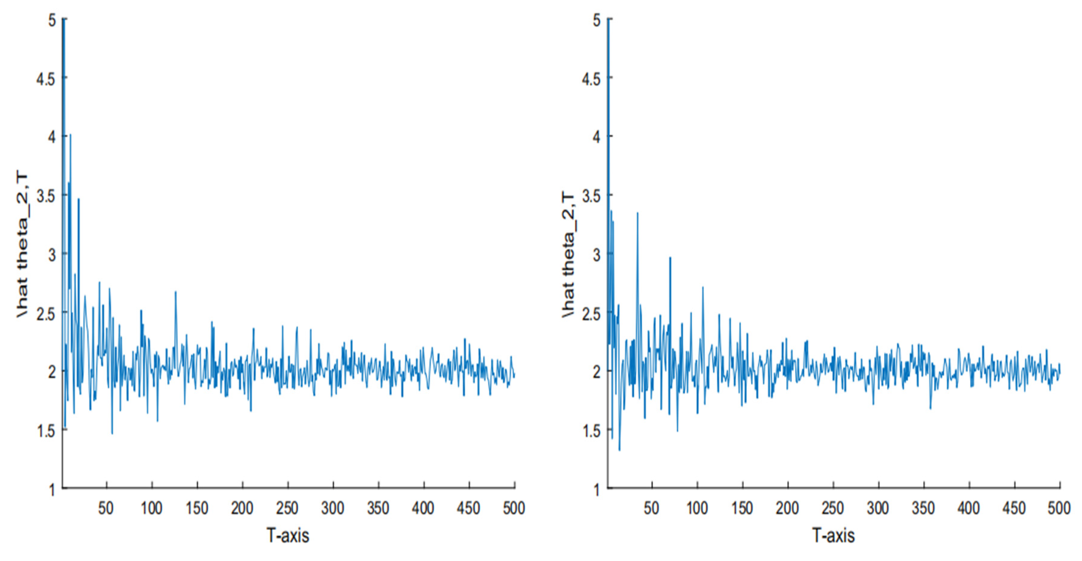
In Figure 1, we let θ 1 = 1 under T = 500, ε = 0.1 and ε = 0.01 ,respectively. In Figure 2, we let θ 2 = 2 under T = 500, ε = 0.1 and ε = 0.01 , respectively. The two figures indicate that when T is fixed and ε is small, the obtained estimators are closer to the true parameter value compared to that of the large ε . When T is large enough and ε is small enough, the obtained estimators are very close to the true parameter value. If we let T convergeto infinity and ε convergeto zero, the two estimators will converge to the true value.

5. Conclusions

The aim of this paper was to study the parameter estimation problem for the Cox–Ingersoll–Ross model driven by small symmetrical α -stable noises from discrete observations. The contrast function was introduced to obtain the explicit formula of the least squares estimators and the error of estimation was given. The consistency and the rate of convergence of the least squares estimators were proved by Markov inequality, Cauchy–Schwarz inequality, and Gronwall’s inequality. The asymptotic distribution of the estimators were discussed as well.

Funding

This research was funded by the National Natural Science Foundation of China under Grant Nos. 61403248 and U1604157.

Conflicts of Interest

The author declares no conflict of interest.The funders had no role in the design of the study; in the collection, analyses, or interpretation of data; in the writing of the manuscript; or in the decision to publish the results.

References

  1. Bishwal, J.P.N. Parameter Estimation in Stochastic Differential Equations; Springer: Berlin, Germany, 2008. [Google Scholar]
  2. Protter, P.E. Stochastic Integration and Differential Equations: Stochastic Modelling and Applied Probability, 2nd ed.; Applications of Mathematics (New York) 21; Springer: Berlin, Germany, 2004. [Google Scholar]
  3. Lauritzen, S.; Uhler, C.; Zwiernik, P. Maximum likelihood estimation in Gaussian models under total positivity. Ann. Stat. 2019, 47, 1835–1863. [Google Scholar]
  4. Wen, J.H.; Wang, X.J.; Mao, S.H.; Xiao, X.P. Maximum likelihood estimation of McKean–Vlasov stochastic differential equation and its application. Appl. Math. Comput. 2015, 274, 237–246. [Google Scholar]
  5. Wei, C.; Shu, H.S. Maximum likelihood estimation for the drift parameter in diffusion processes. Stoch. Int. J. Probab. Stoch. Process. 2016, 88, 699–710. [Google Scholar]
  6. Lu, W.; Ke, R. A generalized least squares estimation method for the autoregressive conditional duration model. Stat. Pap. 2019, 60, 123–146. [Google Scholar]
  7. Mendy, I. Parametric estimation for sub-fractional Ornstein-Uhlenbeck process. J. Stat. Plan. Inference 2013, 143, 663–674. [Google Scholar]
  8. Skouras, K. Strong consistency in nonlinear stochastic regression models. Ann. Stat. 2000, 28, 871–879. [Google Scholar]
  9. Deck, T. Asymptotic properties of Bayes estimators for Gaussian Ito processes with noisy observations. J. Multivar. Anal. 2006, 97, 563–573. [Google Scholar]
  10. Kan, X.; Shu, H.S.; Che, Y. Asymptotic parameter estimation for a class of linear stochastic systems using Kalman-Bucy filtering. Math. Probl. Eng. 2012, 2012, 1–12. [Google Scholar]
  11. Long, H.W. Least squares estimator for discretely observed Ornstein-Uhlenbeck processes with small Levy noises. Stat. Probab. Lett. 2009, 79, 2076–2085. [Google Scholar]
  12. Long, H.W.; Shimizu, Y.; Sun, W. Least squares estimators for discretely observed stochastic processes driven by small Levy noises. J. Multivar. Anal. 2013, 116, 422–439. [Google Scholar] [CrossRef]
  13. Cox, J.; Ingersoll, J.; Ross, S. An intertemporal general equilibrium model of asset prices. Econometrica 1985, 53, 363–384. [Google Scholar] [CrossRef] [Green Version]
  14. Cox, J.; Ingersoll, J.; Ross, S. A theory of the term structure of interest rates. Econometrica 1985, 53, 385–408. [Google Scholar] [CrossRef]
  15. Vasicek, O. An equilibrium characterization of the term structure. J. Financ. Econ. 1977, 5, 177–186. [Google Scholar] [CrossRef]
  16. Bibby, B.; Sqrensen, M. Martingale estimation functions for discretely observed diffusion processes. Bernoulli 1995, 1, 17–39. [Google Scholar] [CrossRef]
  17. Wei, C.; Shu, H.S.; Liu, Y.R. Gaussian estimation for discretely observed Cox-Ingersoll-Ross model. Int. J. Gen. Syst. 2016, 45, 561–574. [Google Scholar] [CrossRef]
  18. Ma, C.H.; Yang, X. Small noise fluctuations of the CIR model driven by α-stable noises. Stat. Probab. Lett. 2014, 94, 1–11. [Google Scholar] [CrossRef]
  19. Li, Z.H.; Ma, C.H. Asymptotic properties of estimators in a stable Cox-Ingersoll-Ross model. Stoch. Process. Appl. 2015, 125, 3196–3233. [Google Scholar] [CrossRef]
  20. Kallenberg, O. Some time change representations of stable integrals, via predictable transformations of local martingales. Stoch. Process. Appl. 1992, 40, 199–223. [Google Scholar] [CrossRef] [Green Version]
  21. Rosinski, J.; Woyczynski, W.A. Moment inequalities for real and vector p-stable stochastic integrals. In Probability in Banach Spaces V; Lecture Notes in Math; Springer: Berlin, Germany, 1985; Volume 1153, pp. 369–386. [Google Scholar]
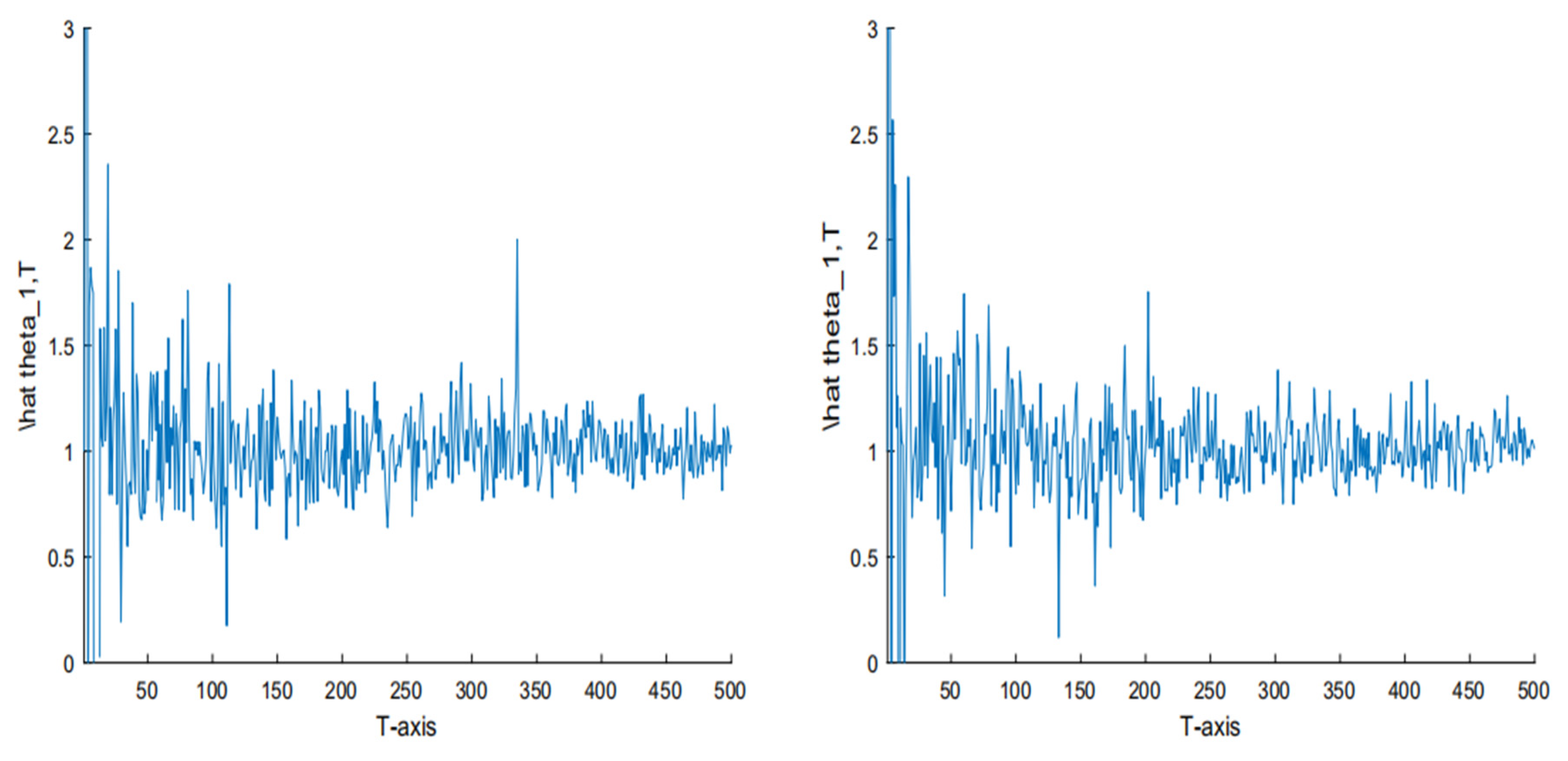
Figure 1. The simulation of the estimator θ 1 ^ , T with T = 500 and θ 1 = 1 under ε = 0.1 and ε = 0.01 , respectively.
Symmetry 12 00327 g001
Figure 2. The simulation of the estimator θ 2 ^ , T and θ 2 with T = 500 and θ 2 = 2 under ε = 0.1 and ε = 0.01 , respectively.
Symmetry 12 00327 g002
Table 1. Least squares estimator simulation results of θ 1 and θ 2 .
True Average AE RE
( θ 1 , θ 2 ) Size n θ 1 L S E θ 2 L S E θ 1 θ 2 θ 1 θ 2
(1,1)10001.26320.75680.26320.243226.32%24.32%
20001.14250.86730.14250.132714.25%13.27%
50001.06510.95860.06510.04146.51%4.14%
(2,3)10001.65733.25380.34270.253817.14%8.46%
20002.18363.12090.18360.12099.18%4.03%
50002.05283.06140.05280.06142.64%2.05%
Table 2. Least squares estimator simulation results of θ 1 and θ 2 .
True Average AE RE
( θ 1 , θ 2 ) Size n θ 1 L S E θ 2 L S E θ 1 θ 2 θ 1 θ 2
(1,1)10,0001.13460.87350.13460.126513.46%12.65%
20,0001.05380.93590.05380.06415.38%6.41%
50,0001.00100.99870.00100.00130.1%0.13%
(2,3)10,0001.86453.14520.13550.14526.78%4.84%
20,0002.06493.07220.06490.07223.25%2.41%
50,0002.00283.00170.00280.00170.14%0.06%