1. Introduction
In recent years, with the rapid development of the economy and society, unconventional oil and gas production, geothermal exploitation, and deep underground space development become major national strategic demands of China [
1,
2]. In these projects, drilling is one of the most basic and extensive operations. Under the influence of deep in-situ stress, the surrounding rock of the wellbore would be deformed and fractured, and three different zones (a damaged zone, a plastic zone, and an elastic zone) would be formed, which have a significant impact on the borehole wall stability [
3,
4]. On the other hand, in-situ stress and geomechanical properties of the surrounding rock mass can also be determined based on the information on rock deformation and failure at a borehole [
5,
6]. In addition, support stress also plays an important role in actual practice [
7,
8]. Therefore, the elastic-plastic-damage analysis of the surrounding rock has important engineering significance.
The elastoplastic analysis of the surrounding rock around a wellbore is a classic fundamental mechanics problem. There are a large number of theoretical, experimental and engineering investigations. In terms of theoretical analysis, in general, it is divided into two major areas:
(1) Considering that the in-situ stress field is a uniform stress field, Fenner simplified the underground circular wellbore into an isotropic plane strain model under uniform force in 1938 and analyzed the stress, strain, and displacement of the ideal elastoplastic rock mass around the wellbore. Based on this model and the rock mass volume constant assumption, Kastner obtained the distribution of the elastic and plastic zones in the surrounding rock, namely the famous Kastner’s Equation [
9], which was followed by many scholars [
10,
11,
12,
13,
14,
15,
16,
17]. The improvement is mainly considering the strain-softening and volume expansion effect of the rock mass. Yuan et al. [
10] considered the softening effect of rock and obtained the distribution of elastic zone, plastic zone and damaged zone in surrounding rock based on Mohr-Coulomb strength criterion. Jiang et al. [
11] simplified the constitutive relationship of the rock in the plastic zone and damaged zone into two horizontal straight lines and obtained the stress and strain of rock mass by non-associative elastoplastic analysis. Sharan [
12,
13,
14] and Park et al [
15] used the elastic-brittle-plastic constitutive model to carry out the elastic-brittle-plastic analysis of circular tunnels based on Hoek-Brown criterion and Mohr-Coulomb criterion, respectively. Zhang et al. [
16] proposed a multi-step brittle-plastic constitutive model to describe the parameter change behavior of the post-peak stage, which was used to carry out the round-hole elastoplastic analysis. Lv et al. [
17] used the elastic-softening-plastic constitutive model of borehole surrounding rock to analyze the stress-strain response around the borehole. The above are all studying the phenomenon of borehole compression, and Li et al. [
18] carried out the elastoplastic calculation of borehole expansion for the hydraulic fracturing problem based on these previous research.
(2) When the circular wellbore is subjected to non-uniform in-situ stress, that is, there is a certain proportional relationship between the vertical and horizontal stresses. In this case, the elastoplastic problem is very difficult to solve, and just approximate solutions were found. In 1946, Galin [
19] first obtained the plastic zone boundary equation and elastoplastic solution of circular holes under non-uniform loads, assuming that the plastic zone near the edge of the hole completely surrounds the hole. The Galin’s solution is widely recognized and used, but the results are only applicable to frictionless Tresca materials. Detournay et al. [
20,
21,
22] then extended the Galin’s solution to the material that accords with cohesive-frictional yield strength and solved the equation of the elastoplastic boundary line by using the complex variable function. The results show that the elastoplastic boundary equation is a Gaussian hypergeometric equation. Ostrosablin [
23] suggested a new method for finding coefficients of the transformation function and gave an example for an accurate solution of determining the plastic zone based on Galin’s solution. Tokar [
24] presented a correction to Galin’s error of omitting the explicit condition for the general balance of forces in bending by means of a modified analytical approach, applying Coulomb’s yield criterion in the plastic zone and assuming continuous or discontinuous stress distributions at the elastoplastic interface. Leitman et al. [
25] presupposed the elastic-plastic boundary is an ellipse and solved a case that Galin’s method cannot solve, in which the plastic domain does not completely surround the hole. Ochensberger et al. [
26] corrected a minor reshaping mistake at the Galin’s solution and provided an amendment to the analytical solution, which was verified by the finite element simulation. Lu et al. [
27,
28] employed the conformal transformation method of complex variable function to map the non-circular elastic regions in the physical plane to the outer regions of the unit circle in the image plane and presented analytical solutions for determination of the plastic zone in the vicinity of a circular tunnel based on the Mohr-Coulomb [
28] or Hoek-Brown failure criterion [
27]. Zhuang and Yu [
29,
30] used the complex variable theory in the elastic analysis to obtain two-dimensional solutions for elastoplastic stress analysis around a cylindrical cavity during both loading and unloading.
In addition, some scholars used approximation methods to solve the elastoplastic problem of circular holes under the non-uniform stress field [
31,
32,
33,
34,
35]. Wei [
31] used the perturbation method to solve the stress in the elastic region, and obtained the elastoplastic zone stress and elastoplastic boundary line equation of the surrounding rock based on Mohr-Coulomb criterion. The results show that the shape of the boundary line of the elastoplastic zone is similar to the ellipse. Hou et al [
32] also used the perturbation method to conduct a similar study on the Drucker-Prager criterion. Chen et al. [
33] substituted the stress analytical solution (Kirsh’s Solution) in the elastic area into the plastic yield condition to obtain the expression and geometry of the elastic-plastic boundary line. Sun et al. [
34] used the stress function obtained by the trial method to solve the elastic stress, and obtained the approximate solution of the plastic zone boundary based on the modified elastic solution. The analytical solutions are valid when the plastic zone is comparatively large and the lateral pressure coefficients 1 ≤
λ < 3. Ma et al. [
35] adopted the stress concentration solution of the circular hole in the elastic plate and the deviatoric stress method in plastic mechanics to solve the problem.
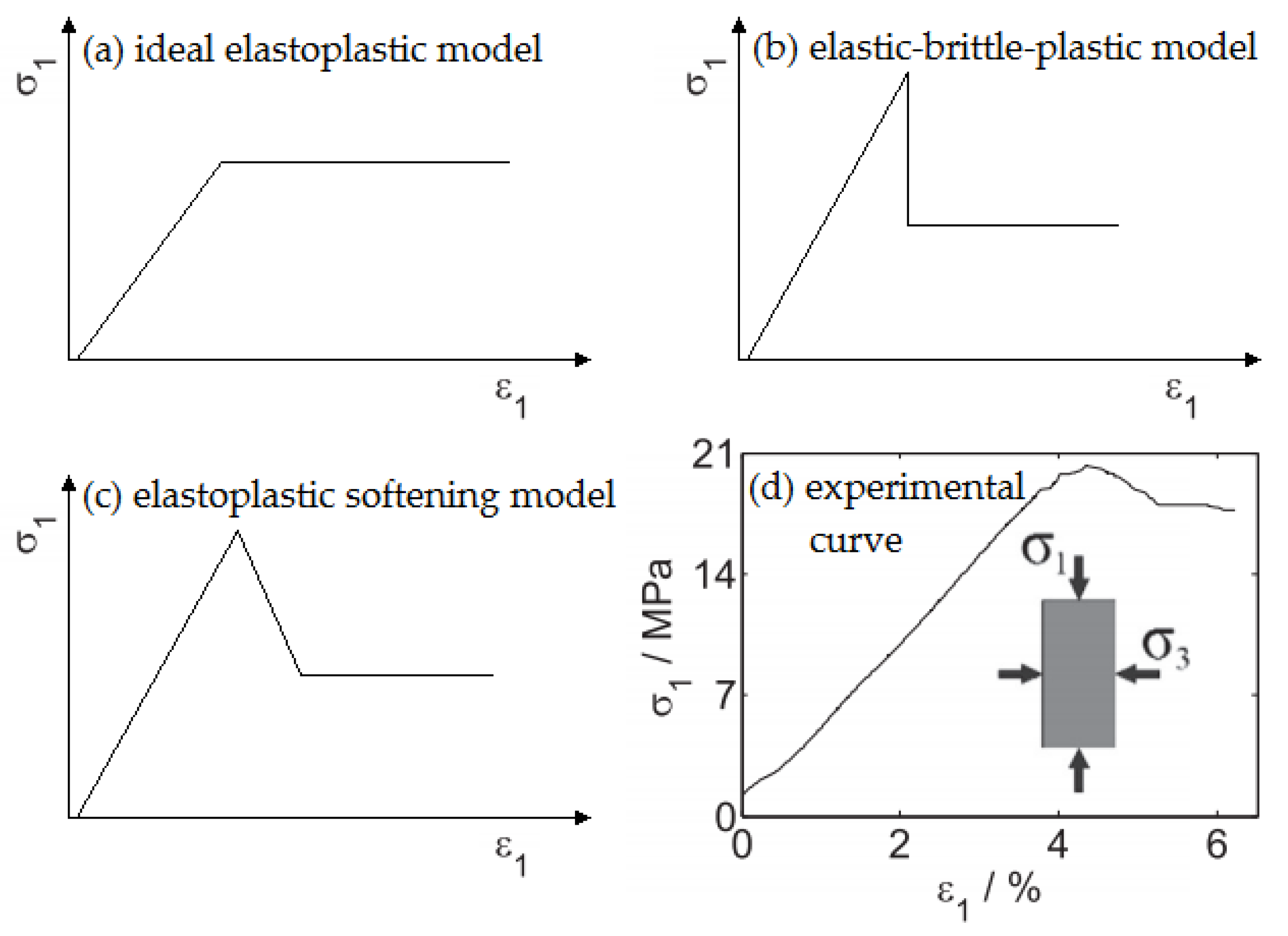
However, as shown in
Figure 1, most of the current research is based on the ideal elastoplastic constitutive model or the elastic-brittle-plastic model, while most of the rocks in engineering practice actually exhibit the strain-softening effect, which is not fully considered in the elastoplastic analysis. In addition, the in-situ stress field is often oversimplified to be uniform. In this paper, the theoretical model describing the elastic-plastic-damaged behavior of strain-softening rock mass around a circular wellbore under the non-uniform in-situ stress field is presented, and the analytical solutions of stress distribution and regional boundary line among elastic zone, plastic zone, and damaged zone are obtained. Then, the influence rules of non-uniform in-situ stress and mechanical parameters on the stress distribution and plastic zone size in surrounding rock mass are analyzed. Finally, comparative analyses are carried out with other solutions.
3. Analytical Solution of Stress and Boundary Line Equation
3.1. Elastic Zone
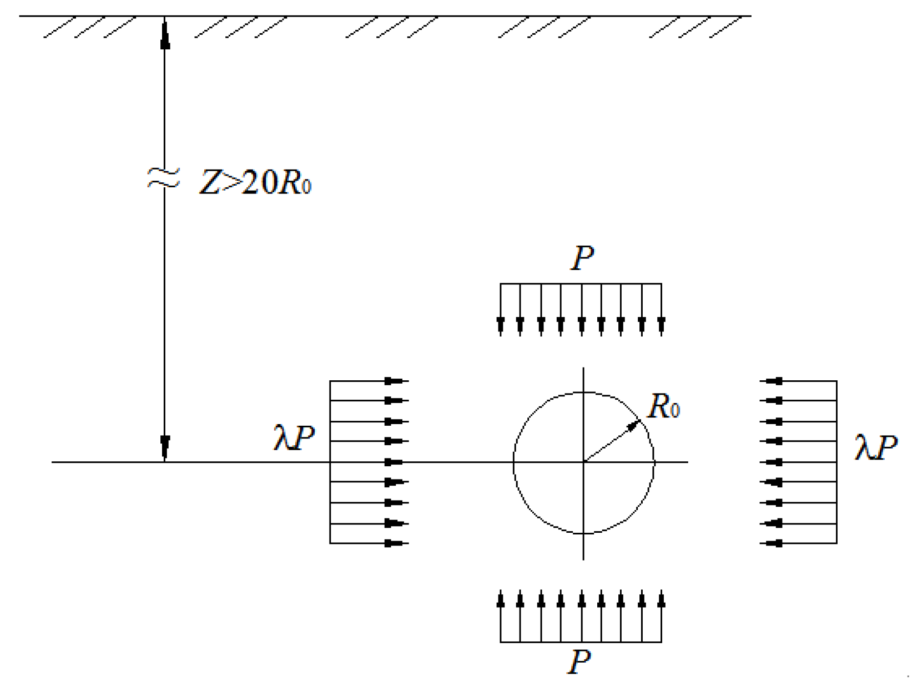
The non-uniform in-situ stress field can be decomposed into a uniform compressive stress field and a two-sided compressive and two-sided tensile stress field, as shown in
Figure 4, so the general form of the stress component of the rock mass in the non-uniform stress field is also the superposition of the two cases.
Figure 4a shows the in-situ stress field,
Figure 4b shows the uniform compressive stress field, and
Figure 4c shows the two-sided compressive and two-sided tensile stress field, and there are
and
.
The general form of the stress in the elastic zone under the uniform compressive stress field is [
10,
36]
where
and
are the radial stress and the hoop stress respectively,
and
are two constants to be determined.
The general form of the stress in the elastic zone under the two-sided compressive and two-sided tensile stress field is [
36]
where
is the shear stress,
and
are pending constants.
By superposing Equation (11) and Equation (12), the general form of the stress component in the elastic zone under the non-uniform in-situ stress field is obtained as
Substituting Equation (14) into Equation (13) and simplifying it, we can get
Applying the boundary condition
Solutions can be obtained that
Substituting Equation (17) into Equation (15), the stress in the elastic zone is obtained as
so at the junction of the elastic and plastic zone, there are
3.2. Plastic Zone
In the plastic softening stage, the Equation (9) is substituted into the equilibrium differential equation for integration and used the boundary condition of stress continuity, that is Equation (19), the stress distribution can be solved.
The equilibrium differential equation in the plastic zone is
Integrate the Equation (20), we can get
where
is a function of
,
is a constant.
Therefore, the hoop stress can be obtained as
Substituting
into Equation (21) and Equation (22), there are
And using the boundary condition, expressed by Equation (19), the radial and hoop stresses in the plastic zone can be solved, which are
3.3. Damaged Zone
The stress component in the damaged zone satisfies the Equation (10), so the equilibrium differential equation in the damaged zone is
There is a certain proportional relationship between the radius of the damaged zone and the plastic zone, which is denoted as
t (
t is not necessarily constant). Substituted this relationship into Equation (9) and used the boundary condition, that is
when
, we can get
Integrate Equation (25) and simplify, there are
where
is the function of
,
is a constant.
Using the boundary condition,
when
, the stress in the damaged zone is
3.4. Boundary Line Equation
There are two boundary lines, the boundary line between the elastic zone and the plastic zone, and the boundary line of the plastic zone and the damaged zone.
It is assumed that the plastic zone of the surrounding rock is completely formed, but the damaged zone is still not produced, which is a critical state. The radius of the plastic zone in this critical state is denoted by
. From Equation (24) and the inner boundary conditions,
and
when
, we can get
In the non-uniform in-situ stress field, the shape of the damaged zone is no longer circular, so it is necessary to classify the above formula to determine whether there is a damaged zone in the surrounding rock. There are four special locations in the damaged zone, that is, the points when
on the inner boundary of the wellbore in the polar coordinates, and the plastic zone ranges in several different cases are discussed below for these four locations.
(a) If , it shows that the surrounding rock is in a critical state that the damaged zone does not appear, there is ,
(b) If
, it is indicated that there is no damaged zone in the surrounding rock, and according to the Equation (9) and Equation (24), as well as the boundary condition,
when
, we can get
Solve the Equation (32) to get the expression of the radius of the plastic zone ,
(c) If , it shows that a local damaged zone is generated in the surrounding rock, that is, the fracture appears on the upper and lower sides of the wellbore, while the left and right sides have not yet broken, and the situation is the most complicated,
(d) If
, it shows that a complete damaged zone is generated in the surrounding rock, that is, the damaged zone completely surrounds the wellbore. Using Equation (28) and the boundary condition,
when
, the radius of the plastic zone can be solved as
The corresponding radius of the damaged zone is . This situation is the most common for deep-buried drilling.
4. Parameter Analysis
Based on the above analytical solutions, we know that the mechanical parameters of the surrounding rock, such as the internal friction angle, cohesion, brittleness coefficient, etc., the lateral stress coefficient, the support force, and other parameters affect the stress distribution and plastic zone size in the surrounding rock. These influence laws are then further analyzed.
4.1. Stress Distribution in Surrounding Rock Mass
Equation (18), Equation (24) and Equation (28) show that the common parameters affecting the stress distribution in the three zones are the internal friction angle, the cohesion, and the lateral stress coefficient. In order to make the results more intuitive, the stress at the line θ = 60° is representatively selected as the research object.
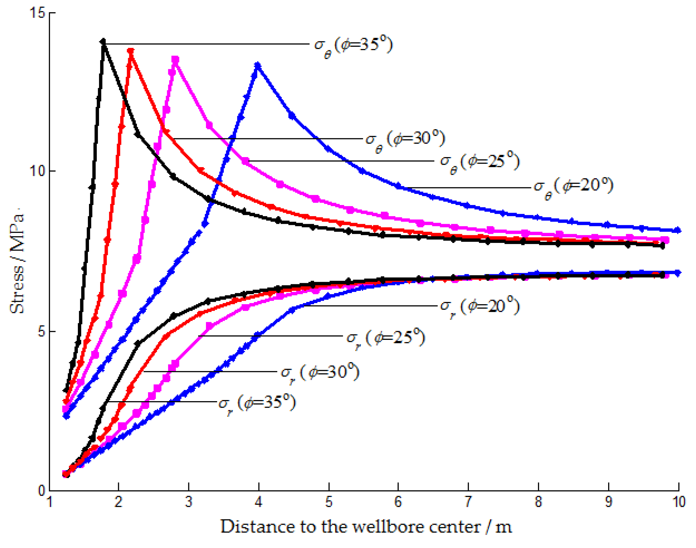
4.1.1. Effect of the Internal Friction Angle
The mechanical parameters of surrounding rock at Nantun mine in Shandong Province in
Table 1 are utilized, and the internal friction angles are taken as 20°, 25°, 30°, and 35°, respectively. Substituting these data into the Equation (18), Equation (24) and Equation (28), and the radial and hoop stresses in the surrounding rock mass can be calculated, shown in
Figure 5.
It can be seen from
Figure 5 that the hoop stress is always larger than the radial stress. The maximum hoop stress appears at the interface between the elastic and plastic zones, and the stress concentration factor is about 2. In the plastic and the damaged zones, the hoop stress gradually increases with increasing distance to the wellbore, while in the elastic zone, it decreases to approximately the in-situ stress with the distance trending to infinity. In sharp contrast, the radial stress keeps increasing smoothly with distance to the wellbore, which means that it is continuous in the surrounding rock mass, even passing through the interface between the different zones [
18]. As the internal friction angle increases, the maximum hoop stress increases slightly, and the location is closer to the wellbore. In addition, in the plastic and the damaged zones, both the hoop and radial stresses and their gradients become larger.
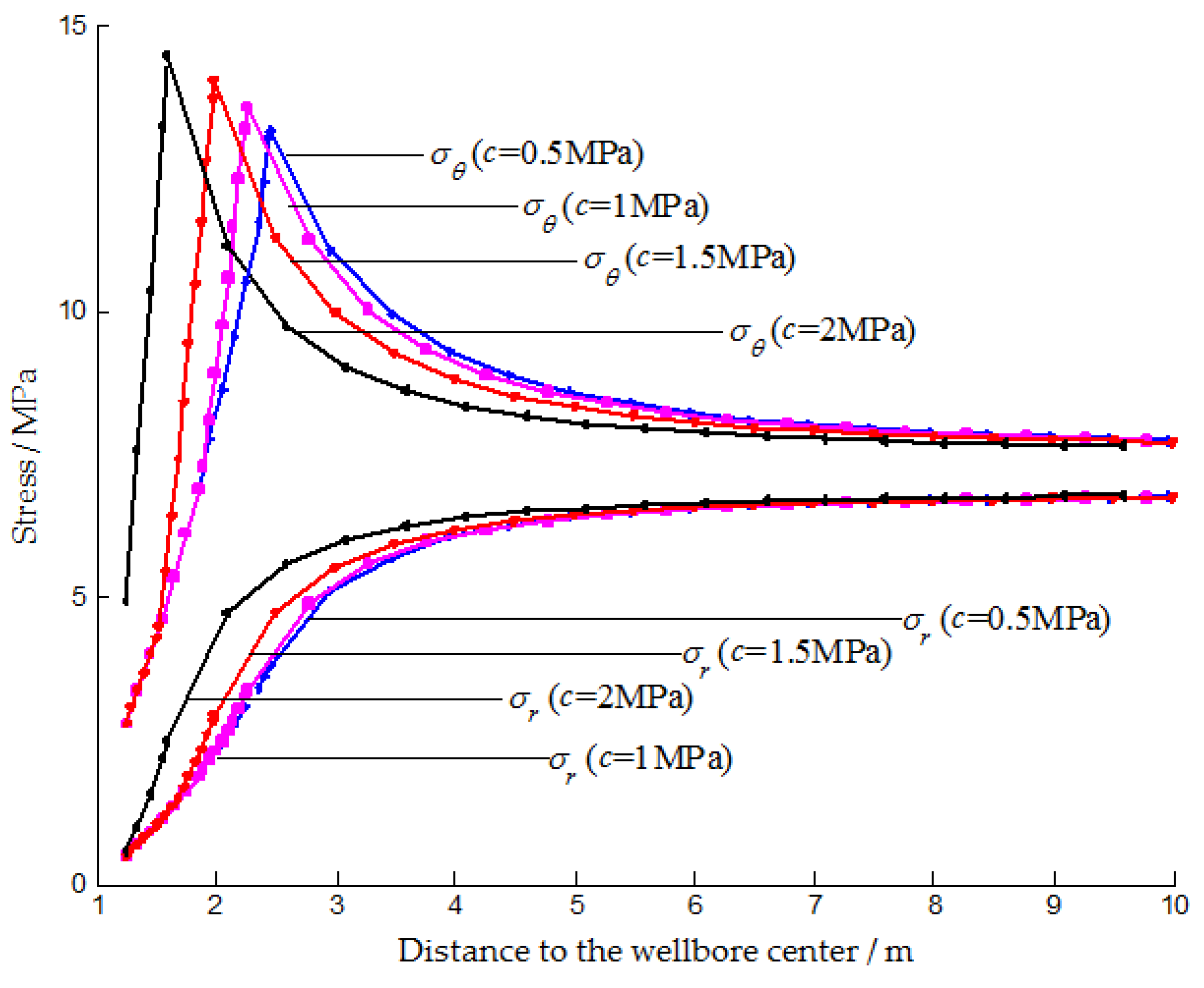
4.1.2. Effect of the Cohesion
The data in
Table 1 are also utilized, and the cohesion is taken as 0.5 MPa, 1 MPa, 1.5 MPa, and 2 MPa, respectively. Based on Equation (18), Equation (24) and Equation (28), the radial and hoop stresses can be also calculated, as seen in
Figure 6.
Figure 6 shows that when the cohesion is larger, the maximum hoop stress is larger and the distance between its location and the wellbore is smaller. The radial stress is always in the increasing trend. These laws are similar to those in
Figure 5, but the difference in stress values under different cohesion is not so large, which means the stress distribution is less sensitive to cohesion than the internal friction angle. At a distance greater than 5 m from the wellbore, the effect of cohesion on stress is very weak.
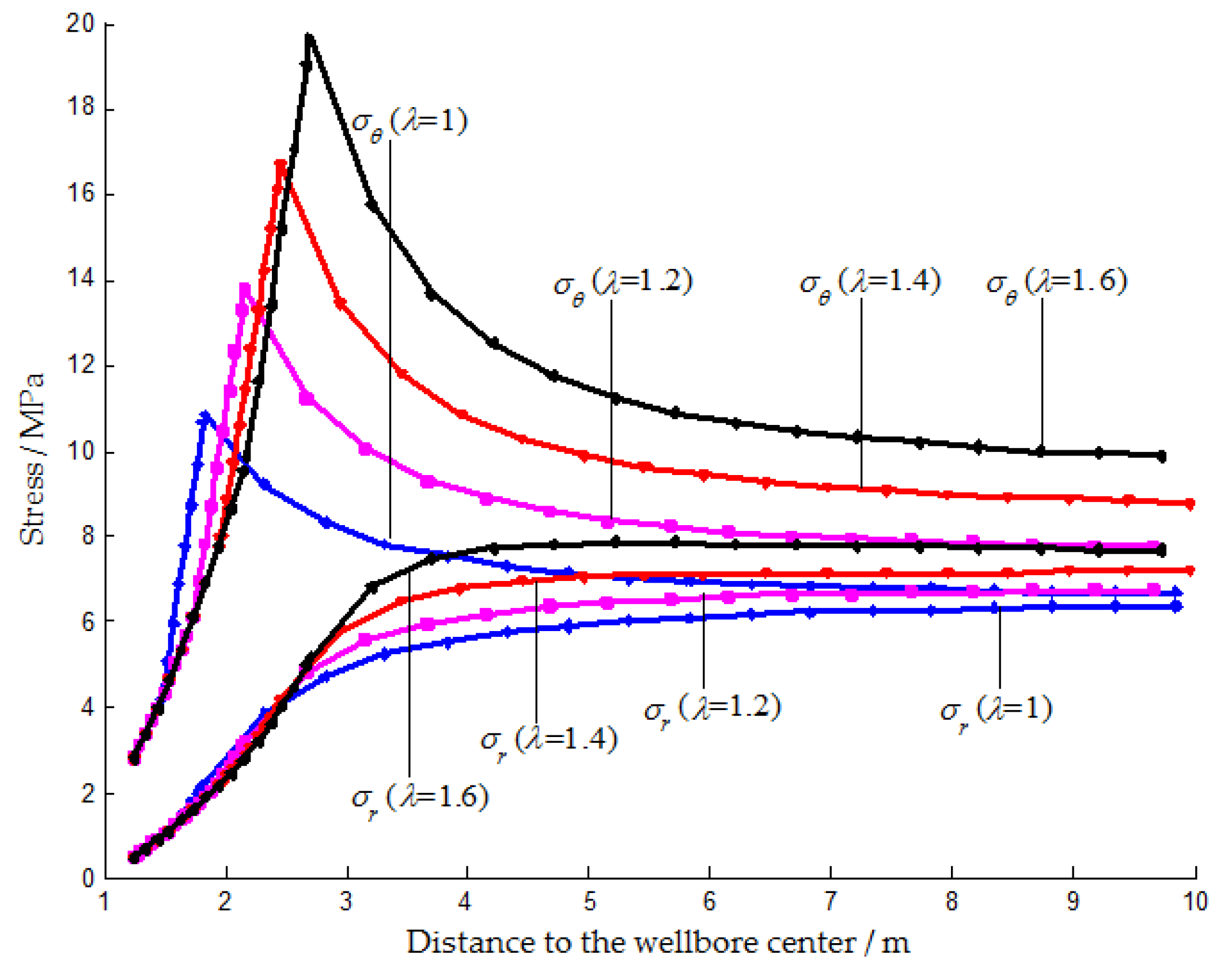
4.1.3. Effect of the Lateral Stress Coefficient
Similarly, the lateral stress coefficient is taken as 1, 1.2, 1.4, and 1.6, respectively. The calculation results can show the effect of the lateral pressure coefficient on the stress distribution in the surrounding rock mass, seen in
Figure 7.
The lateral pressure coefficient has a significant effect on the stress distribution in the three regions, as shown in
Figure 7. As it increases, the stress concentration becomes stronger, the maximum hoop stress and radial stress both increases significantly, and the boundary between the plastic and elastic zones moves farther away from the wellbore. It is also interesting to observe that the stress curves in the same area are close to parallel under different lateral stress coefficients, which seems to mean that the lateral stress coefficient only affects the stress value without affecting the stress gradient.
4.2. Size of the Plastic Zone
Determining the size of the plastic zone in the surrounding rock mass plays an important role in controlling the stability of the wellbore. According to Equation (33), we can know that multiple parameters collectively affect the size of the plastic zone, including internal friction angle, cohesion, residual strength, in-situ stress, support force, lateral stress coefficient, brittleness coefficient, well radius, etc. Here, we mainly analyze four factors as follows.
Taking the data listed in
Table 1 as reference parameters, when discussing the influence of a certain factor on the radius of the plastic zone, only change the value of this parameter, while other parameters are kept unchanged. Since the boundary of the plastic zone is symmetrical in all four quadrants, only a quarter of the curve is drawn from 0° to 90°, and the radius of the plastic zone at other angles can be obtained through the symmetry relationship.
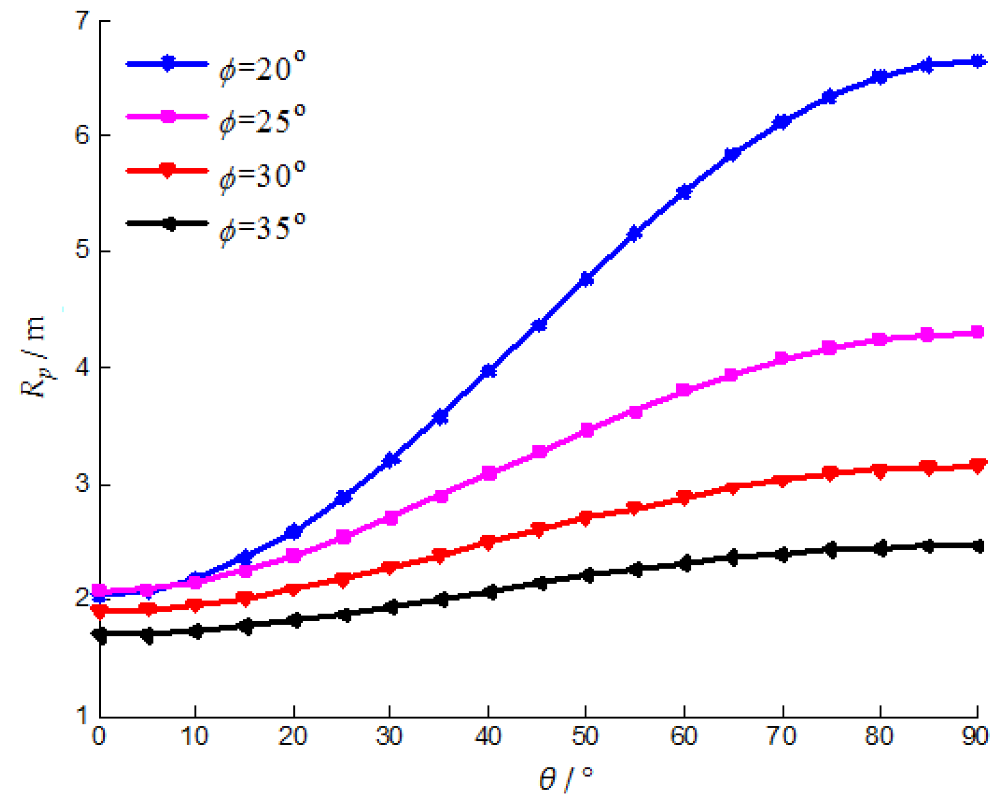
4.2.1. Effect of the Internal Friction Angle
Taking the internal friction angles as 20°, 25°, 30°, and 35°, and substituting them into the expression of the radius of the plastic zone shown in Equation (33), a series of values of the radius of the plastic zone changing with the angle
θ are obtained, which can be shown by the curves in
Figure 8.
As can be seen from
Figure 8, the effect of the internal friction angle on the radius of the plastic zone is quite significant. As the internal friction angle increases, the radius of the plastic zone decreases at all locations, but the magnitude of the reduction is different. The radius of the plastic zone decreases the least at
θ = 0°, and decreases most at
θ = 90°. The difference in the radius of the plastic zone at each location is gradually decreasing with the increasing internal friction angle, that is, the shape of the plastic zone is getting closer to a circle.
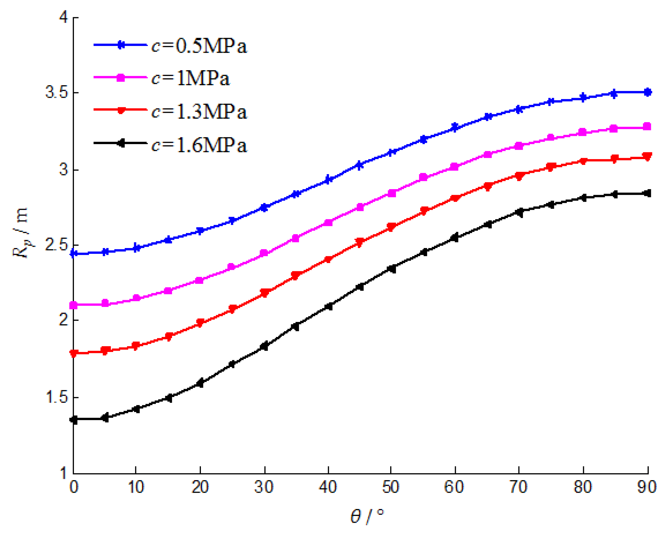
4.2.2. Effect of the Cohesion
Take the cohesion as 0.5 MPa, 1 MPa, 1.3 MPa, and 1.6 MPa respectively, and draw the calculated plastic zone radius value, then the curves of the radius of the plastic zone as a function of the cohesion can be obtained, shown in
Figure 9. Similar to the influence of the internal friction angle in
Figure 8, the radius of the plastic zone decreases with increasing cohesion. However the difference is that the amplitude of the reduction at the position of
θ = 0° is greater than that at
θ = 90°, which means that the plastic zone is becoming flattened.
4.2.3. Effect of the Brittleness Coefficient
The brittleness coefficient characterizes the degree of strain-softening of the rock mass and can be expressed by Equation (2). Take the brittleness coefficient as 0.3, 0.5, 0.8, 1.2, 5, 10, 15, 30 in order, and draw the curves of the plastic zone radius with the brittleness coefficient, as shown in
Figure 10.
The radius of the plastic zone increases with the increase of the brittleness coefficient, and the difference of the increased amplitude at each location is small, which means that the plastic zone is enlarged approximately in proportion. A very significant feature is that when the brittleness coefficient is small (
β < 5), as shown in
Figure 10a, as the brittleness coefficient increases, the gradient of the increase in the radius of the plastic zone becomes smaller and smaller. When it is large (
β > 5), the radius of the plastic zone hardly increases, and the plastic zones almost coincide, as shown in
Figure 10b.
4.2.4. Effect of the Lateral Stress Coefficient
Take the lateral pressure coefficient as 0.8, 1.1, 1.2, and 1.3 in order, and draw the curves of the plastic zone radius with the lateral pressure coefficient, as shown in
Figure 11.
The influence of the lateral pressure coefficient on the radius of the plastic zone is very significant. When λ < 1, that is, the vertical stress is higher than the horizontal stress, the radius of the plastic zone decreases with increasing angle, which means that the plastic zone is long in the horizontal direction and short in the vertical direction. The situation is reversed when λ > 1. There is a clear demarcation point, which is around θ = 37°. With the increase of the lateral stress coefficient, the changing trend is opposite on both sides of this demarcation point, the radius of the plastic zone becomes larger in the region of θ > 37°, but smaller in θ < 37° section. The difference between the radius of the plastic zone at θ = 0° and θ = 90° is getting bigger, which means that the plastic zone is getting flatter.
5. Comparison of Results
The deformation and fracture behavior of the rock mass around the borehole is mainly affected by the in-situ stress and the mechanical properties of the surrounding rock. The present model solves the stress and plastic zone distribution in the elastoplastic softening rock mass under the non-uniform in-situ stress, and it can degenerate into solutions under simple conditions after modifying some parameters. When
λ = 1, it becomes the case under uniform in-situ stress, and the obtained result is completely consistent with Yuan Wenbo’s Solution [
10], if
β = 0, the model becomes the Kastner’s Equation further [
9]. Next, the present model is compared with two special cases (using the elastoplastic softening model under a uniform stress field, using the ideal elastoplastic model under a non-uniform stress field) and an approximation method with high precision (the perturbation method) to highlight its characteristics.
5.1. Comparison with the Results Using the Elastoplastic Softening Model under Uniform Stress Field
It can be known from Equation (33) that if the mechanical parameters of the surrounding rock are determined, the radius of the plastic zone is only a function of the angle θ, so the shape of the boundary line between the elastic zone and plastic zone is no longer a circle. Furthermore, the radius of the plastic zone is a function of cos2θ, and it is related to the lateral stress coefficient λ.
According to the in-situ stress and mechanical parameters of the surrounding rock at Nantun mine in Shandong Province (seen in
Table 1), substituting them into the Equation (26) and Equation (33), the area and the shape of the plastic zone and the damaged zone around the wellbore under the non-uniform stress field and the uniform stress field can be calculated, shown in
Figure 12.
It can be seen from
Figure 12 that when the lateral stress coefficient
λ > 1, that is, the horizontal stress is greater than the vertical stress, the plastic zone and the damaged zone are both approximately elliptical, short in the horizontal direction and long in the vertical direction, and have concaves on the left and right sides. Compared with the case of uniform stress field (
λ = 1) [
10,
11,
16,
17,
18], the plastic and fracture area on the left and right sides of the wellbore become significantly smaller, while that on the upper and lower sides increase. It can be predicted that, when
λ < 1, that is, the horizontal stress is less than the vertical stress, the plastic area on the left and right sides of the well is larger than that on the upper and lower sides, and the damaged zone is also the same.
5.2. Comparison with the Results Using the Ideal Elastoplastic Model under Non-Uniform Stress Field
The selection of the constitutive model of the surrounding rock has a great influence on the results. In this part, the elastoplastic softening model and the ideal elastoplastic model are compared. Considering the Mohr-Coulomb criterion is adopted for the yield of the surrounding rock, so the comparison is performed under different values of internal friction angle and cohesion.
5.2.1. Effect of the Internal Friction Angle
Similarly, the surrounding rock parameters in
Table 1 are used, and the internal friction angles are taken as 20°, 25°, 30°, and 35°, respectively, and the different two models are substituted to solve the shape of the plastic zone, as shown in
Figure 13.
It can be seen from
Figure 13 that the plastic zone under the elastoplastic softening model is concave on the left and right sides, while it is approximately elliptical under the ideal elastoplastic model. The plastic zone size difference between the two models is significant. On the left and right sides of the well (the angle is 0° or 180°), the radiuses of the plastic zones calculated by the two models are close, and the gap increases with the angle. It is getting bigger and bigger until the upper and lower sides reach the maximum. In addition, with the increase of the internal friction angle, the radius of the plastic zone under the two models decrease to different extents, and the difference between them becomes smaller and smaller.
The reason is that the stress in the plastic deformation stage of the ideal elastoplastic model remains constant and is greater than the stress in the elastic stage. The rock mass in the plastic zone can still maintain a stable state under the in-situ stress so that the boundary of the plastic zone would not change suddenly, and thus the shape of the plastic zone is relatively regular [
26,
27,
28]. However, in the elastoplastic softening model, when the stress exceeds the compressive strength of the rock mass, the strain-softening effect will reduce the strength. The strength of the rock mass at different positions is different, and thus the deformation is different. Therefore, the boundary shape of the plastic zone is irregular. Specifically, the plastic zone on the left and right sides of the wellbore is concave, and this tendency tends to increase as the lateral stress coefficient increases.
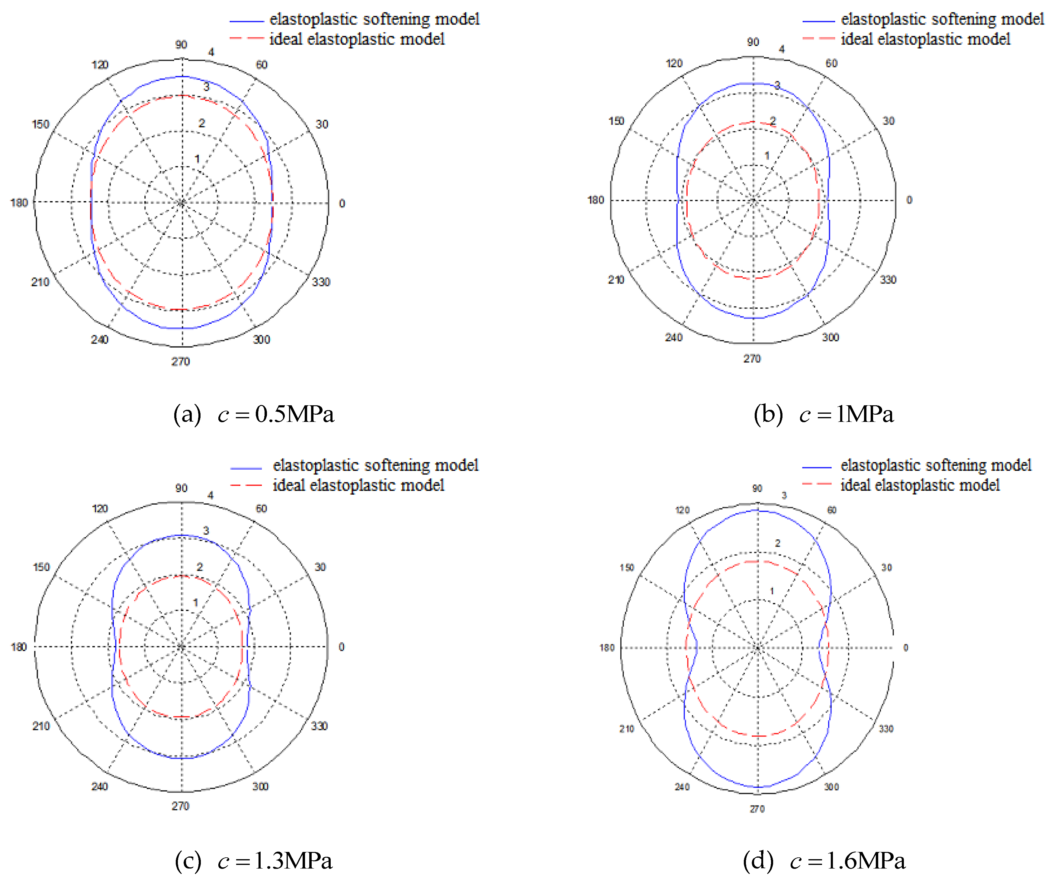
5.2.2. Effect of the Cohesion
The surrounding rock parameters in
Table 1 are still used, and the cohesive is taken as 0.5 MPa, 1 MPa, 1.3 MPa, and 1.6 MPa, respectively, and the different two models are substituted to solve the shape of the plastic zone, as shown in
Figure 14.
It can be seen from
Figure 14 that as the cohesion increases, the radius of the plastic zone under the two models decreases, and the difference between them increases. The plastic zone shape under the ideal elastoplastic model is always approximately elliptical, under the elastoplastic softening model it changes from approximately elliptical to concave on the left and right sides. In general, the area of the plastic zone calculated by the elastoplastic softening model is larger than that by the ideal elastoplasticity model.
As can be seen from
Figure 13 and
Figure 14, the internal friction angle and the cohesion significantly affect the difference between the calculation results of the two models. The internal friction angle of the rock mass characterizes the frictional effect, including the sliding friction caused by the surface roughness of the mineral particles when they mutually slip, and the occlusal friction caused by the movement of the mineral particles in the state of embedding, interlocking and detachment. The larger internal friction angle leads to the more significant friction effect of the rock mass, and the concave phenomenon in the plastic zone will be weakened. Cohesion is the mutual attraction between adjacent parts of a substance, which is the expression of molecular forces. In the case of effective stress, the cohesion is obtained by subtracting the total shear strength from the friction strength. Therefore, as the cohesion increases, the concave phenomenon in the plastic zone will be enhanced. In general, the increasing internal friction angle and cohesion will enhance the shear strength of the surrounding rock, so the plastic zone area around the wellbore will gradually decrease.
5.3. Comparison with the Results of the Perturbation Method
The perturbation method, also known as the small parameter expansion method, is a method for solving the mathematical physics problem with high precision [
31,
32]. Since the solution using the perturbation method in the existing literature is based on the ideal elastoplastic model of the rock mass, in order to facilitate the comparison, some parameters in the present model need to be changed to transform into a special one under the ideal elastoplastic model. Make the corresponding change to the Equation (33), that is, substituting
and
into the equation, the radius of the plastic zone becomes
The radius of the plastic zone obtained by the perturbation method is [
31]
According to the form of the above two equations, Equation (34) and Equation (35), it is difficult to visually see the difference in the shape of the resulting curves. Therefore, the specific parameters in
Table 1 are still used for calculation. Considering the influence of the mechanical properties of the surrounding rock, they are compared under different internal friction angles and cohesion, as shown in
Figure 15.
It can be seen from
Figure 15 that the area of the plastic zone obtained by the two methods is basically the same, and the relative error is within 5%. In terms of the shape of the plastic zone, the curve calculated by the perturbation method is more elliptical, while it is slightly slender by the proposed method, that is, the plastic zone size on the left and right sides of the wellbore is smaller than that obtained by the perturbation method, and it is bigger on the upper and lower sides.
From the principle of the perturbation method and the expression of the radius of the plastic zone, it is basically a correction to the Kastner’s equation [
9]. When
λ = 1 is taken in Equation (35), the Kastner’s equation can be obtained [
32]. Therefore, the shape of the plastic zone obtained by the perturbation method is theoretically approximately elliptical and will become closer to a circle when certain conditions are met. However, the proposed model is based on the premise of the non-uniform in-situ stress field, and the elastoplastic softening model is adopted, so it has certain advantages since the perturbation method cannot solve such problems.
It is worth noting that there is another approach to solve the stresses and the displacements around a borehole, that is, by assuming that Young’s modulus varies around a circular opening according to a given function, which arises from strain-induced damage or from confining stress effects in a material with stress-dependent stiffness, a radius-dependent modulus (RDM) model was proposed to quantify the concept of a variably damaged zone around an opening [
37]. Compared with the present model, the RDM model is mathematically simpler and easier to calculate, but the chosen Young’s modulus function would bring more uncertainty to the calculation result, and a closed-form solution cannot be obtained. In addition, the RDM model cannot distinguish between the plastic zone and the damaged area. From the calculation results of stress distribution, as shown in
Figure 5,
Figure 6 and
Figure 7, the two models are similar that the hoop stress reduces at the borehole wall and reaches a maximum at some distance from the wall, while the radial stress increases monotonically with distance to the borehole. More detailed comparative studies will be conducted in the future.
6. Conclusions
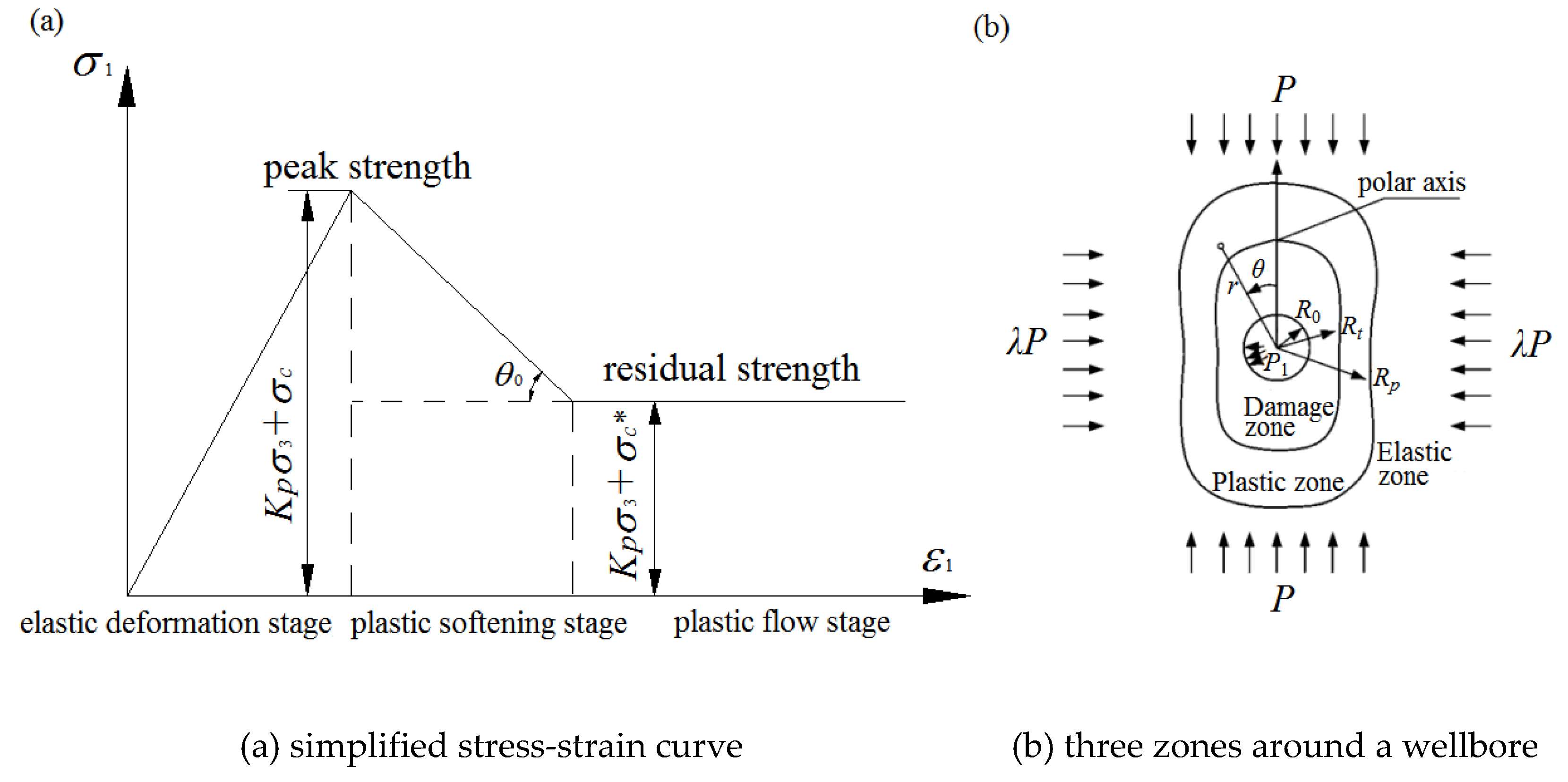
In this study, based on the elastoplastic softening model of rock and the Mohr-Coulomb strength criterion, the stress distribution of elastic zone, plastic zone and damaged zone in the surrounding rock of a circular wellbore is obtained by the in-situ stress field decomposition method, and the boundary line equations of the plastic and damaged zone are further obtained. Then, the influence rules of lateral stress coefficient and mechanical parameters on the stress distribution and plastic zone size in surrounding rock mass are analyzed. Finally, the proposed model is compared with the cases of the uniform in-situ stress field, the ideal elastoplastic model and the perturbation method. The main conclusions are as follows:
(1) The proposed model solves the stress and the plastic-damaged zone distribution in the elastoplastic softening rock mass in the non-uniform in-situ stress field. After modifying the model parameters, it can be degraded into solutions under simple conditions. When , it becomes the case of a uniform in-situ stress field, and the obtained result is completely consistent with Yuan Wenbo’s Solution. If , then the model is transformed into Kastner’s Equation.
(2) The effect of the non-uniform in-situ stress field: As the lateral stress coefficient increases, the stress concentration becomes stronger, the maximum hoop stress and radial stress both increase significantly. The shape of the plastic zone and the damaged zone under the uniform in-situ stress is circular, but under the non-uniform in-situ stress, it becomes an approximately elliptical shape and getting flatter with increasing lateral stress coefficient.
(3) The effect of the mechanical properties of the surrounding rock: As the internal friction angle and the cohesion increase, both the hoop and radial stresses and their gradients become larger, and the area of the plastic zone is significantly reduced. The plastic zone increases approximately proportionally with the increasing brittleness coefficient, and finally reaches a stable value. When the brittleness coefficient is greater than 5, it almost never increases.
(4) Comparison with the perturbation method: The plastic zones obtained by the present method and the perturbation method are basically the same when the ideal elastoplastic model is adopted. However, the perturbation method cannot solve the problem in the elastoplastic softening rock mass under the non-uniform in-situ stress field.


