1. Introduction
The presence of rotating objects in electromagnetic problems is of interest in several applications, ranging from the detection of helicopters to the tachometry of celestial bodies [
1,
2]. Unfortunately, as an immediate consequence of the presence of materials in motion, all these electromagnetic problems are difficult to solve. This is a consequence of the fact that all moving media are perceived as bianisotropic [
3,
4].
Independently of the motion, bianisotropic media have been considered in several recent investigations, in particular in the context of metamaterials, with frequencies belonging to the microwave band or to the photonic one [
5,
6,
7,
8], for their huge potentialities or for their practical applications.
The complexity of electromagnetic problems involving media in motion or bianisotropic materials prevents any chance of getting results without the use of numerical simulators. However, in order to rely on them, it is important to know a priori results of well posedness of the problems of interest and on their numerical approximability. A few papers addressing these topics have been recently published [
9,
10,
11,
12]. However, due to the difficulty of the problems considered, most of them present results under some restrictive hypotheses. For example, in [
9], the results of interest are deduced by exploiting in a crucial way the presence of losses, while in [
10] the authors study cylinders in axial motions. In [
11], a problem of evolution is studied inside a cavity, preventing the exploitation of the results in many applications and, finally, in [
12] the constitutive parameters are smooth so neglecting the possibility of considering radiation or scattering problems.
In this paper, we try to overcome most of these limitations by extending the theory developed in [
10] to three-dimensional time-harmonic electromagnetic boundary value problems involving lossy or lossless materials which can be bianisotropic or in motion. Only on the materials in motion will we consider some restrictions. In particular, in order to retain the possibility to perform the analysis of time-harmonic problems, we need that the boundaries of the moving objects are stationary [
3]. Thus, we will restrict ourselves to consider the rotation of axisymmetric objects. For the same reason, the velocity field will be considered independent of time. Moreover, the media in motion have to be non-conductive, in order to avoid the difficulties related to the convective currents, which could become surface electric currents [
13] and then determine a discontinuity of the tangential part of the magnetic field.
As for the media involved whose bianisotropy is not due to motion, we do not consider any restrictive hypothesis. In particular, the formulation we consider allows the solution of radiation [
14], scattering [
1,
5,
15], or guided wave problems [
16,
17], which are all of interest for applications.
The well posedness and finite element approximability guaranteed by our theory allow us to obtain reliable solutions from numerical simulations for rotating axisymmetric objects. With this, we can solve several problems. However, for the sake of conciseness, we selected just two representative examples. For one of them, we have approximate semi-analytic solutions [
1], and the range of validity of the approximation involved in those solutions can be verified using our approach. Our second example is representative of the majority of problems involving rotating objects, for which no result can be found in the open literature. For any problem of this class, the reliable solution obtained under the conditions required by our theory can serve as a benchmark for other numerical techniques.
The paper is organized as follows. In
Section 2, the problems of interest are defined.
Section 3 reports the main ideas which can be used to show that the problems of interest are well posed. The results of convergence of Galerkin and finite element approximations are presented in
Section 4. In
Section 5, we briefly present the main features of the finite element simulator exploited to compute the results presented in
Section 7. In these first sections, we heavily exploit the results presented in [
9,
10,
18]. We have included these sections in our manuscript in order to ease readers’ task and because the results we present are not trivially deduced from [
10,
18], since they deal with two-dimensional problems. The main novelties of the paper are presented in
Section 6 and
Section 7. In particular, in
Section 6, we present some useful suggestions on how our theory can be exploited to solve problems of practical interest and in
Section 7 the practical applications of our theory to rotating axisymmetric objects are presented. The conclusions are reported in
Section 8 and some technical details are provided in the appendix.
2. Problem Definition
In this section, we define the time-harmonic electromagnetic boundary value problem we will deal with in the rest of the paper. Most of the considerations of this section are taken from Sections 2 and 3 of [
9] and are here reported to ease the reader’s task and to introduce some specific considerations of interest for problems involving rotating axisymmetric objects.
To avoid restrictions on the applicability of our analysis, the problem will be formulated on a domain satisfying the following hypotheses ( denotes its boundary):
- HD1.
is open, bounded and connected,
- HD2.
is Lipschitz continuous and stationary.
Moreover, in order to be able to consider electromagnetic problems of practical interest, different inhomogeneous materials will be taken into account. This is the reason why we assume:
- HD3.
can be decomposed into m subdomains (non-empty, open and connected subsets of having Lipschitz continuous stationary boundaries) denoted , , satisfying ( is the closure of ) and for .
This hypothesis allows us to consider also the presence of rotating axisymmetric objects.
The specific target of the paper is to deal with electromagnetic problems involving very general materials. However, in order to give a sense to a time-harmonic analysis, we have at least to assume that:
- HM1.
Any material involved is linear and time-invariant and satisfies the following constitutive relations:
In the above equation,
,
,
,
, and
are, respectively, the electric field, the magnetic induction, the electric displacement, the magnetic field and the velocity of light in vacuum [
19].
L,
M,
P and
Q are four 3-by-3 matrix-valued complex functions defined almost everywhere in
. The vector fields
,
,
and
are complex valued too, as it is usually the case for electromagnetic field problems in which the real fields depend sinusoidally on time [
20] (pp. 13–16). Equation (
1) implicitly takes account of the electric current densities, as usual. Other equivalent forms of the above constitutive equations are possible [
21] (p. 49) [
22], and will also be used later on.
Different inhomogeneous bianisotropic materials will be modeled by assuming the following hypothesis.
- HM2.
The matrix valued complex functions representing the effective constitutive parameters satisfy [
23] (p. 3), [
24] (p. 36):
Such hypothesis is in no way restrictive for all applications of interest since the material properties are just piecewise but not globally continuous. In particular, as we will verify later on, hypotheses HM1 and HM2 do not exclude the presence of rotating axisymmetric objects [
2] either.
The following additional notations and hypotheses are necessary too.
is the usual Hilbert space of complex-valued square integrable vector fields on
and with scalar product given by
(
denotes the conjugate transpose).
[
24] (p. 55). The space where we will seek
and
is [
24] (p. 82; see also p. 69)
where [
24] (p. 48)
The scalar products in
and
U are respectively given by
and [
24] (p. 84, p. 69)
The induced norm is .
The symbol represents the angular frequency, as usual. Moreover, and are the electric and magnetic current densities, respectively, prescribed by the sources, Y is the scalar admittance involved in impedance boundary condition and is the corresponding inhomogeneous term. Finally, the admittance function Y with domain and range in is assumed to satisfy
- HB1.
Y is piecewise continuous and is bounded.
We are now in a position to state the electromagnetic boundary value problem we will address in this paper.
Problem 1. Under the hypotheses HD1-HD3, HM1-HM2, HB1, given , , and , find satisfying (1) and the following equations: As it was pointed out in [
9], such a model can be thought of as an approximation of a radiation or scattering problem, or as a realistic formulation of a cavity problem.
The following variational formulation of Problem 1 was derived in [
9]:
Problem 2. Under the hypotheses HD1–HD3, HM1–HM2, HB1, given , , and , find such that
where
and
It was shown in [
9] that the two formulations are equivalent, in the sense that, from the solution of Problem 1, one can deduce the solution of Problem 2 and vice versa; moreover, the well posedness of the former implies the well posedness of the latter and vice versa [
9].
3. Well Posedness of the Problem
Following the main ideas presented in Section 4 of [
10], in this section, we prove the well posedness of the three-dimensional problems of interest. The target will be achieved by showing that, under appropriate additional hypotheses, we can apply the generalized Lax-Milgram lemma [
24] (p. 21) to Problem 2.
The continuity of the sesquilinear and antilinear forms,
a and
l, are easily deduced under the hypotheses already introduced (HD1-HD3, HM1-HM2, HB1). Thus, it remains to introduce the additional hypotheses allowing us to prove that the sesquilinear form
a satisfies the following conditions:
We establish under which hypotheses these conditions hold true in the following subsections.
3.1. Hypotheses to Prove Condition (9)
Condition (
9) is easily proved once we know that the solution to Problem 2 is unique, as shown in [
10]. In turn, uniqueness for Problem 2 is achieved by proving uniqueness for the corresponding homogeneous problem (that is the one with
) [
25] (p. 20), [
24] (p. 92). Finally, uniqueness for the corresponding homogeneous problem can be deduced by a standard technique [
26] (pp. 187–203), [
10,
24,
27] (p. 92), in the presence of some losses and by unique continuation results.
In the following, we introduce the hypotheses which allow for getting the result of interest in this subsection. In order to let the reader understand the general picture, we observe that:
the first group of hypotheses (HM3 and HB2) requires that the media and the boundary do not provide active power,
the second group of assumptions (HM4–HM7 and HB3) asks for the presence of some losses in the media or on the boundary or the invertibility of the constitutive matrix P, ,
the first two groups of hypotheses are sufficient to prove that the solution of the homogeneous problem is zero on a subdomain of or that its tangential part on a subset of the boundary is zero,
the third group of assumptions (HM8–HM12) guarantee the applicability of a unique continuation result, allowing us to show that condition (
9) holds true.
In order to write our assumptions, we need to introduce some additional notation.
In [
9], it was shown that the sesquilinear form
a can be recast is the form
where
being [
9]
and
. For future use, the vector notation introduced in Equation (
11) is generalized as follows for the ordered pair
:
Moreover, by referring to the constitutive relation (
1) or the above definition of
A, we introduce a splitting of the subscript
of the subdomains
:
when
(the media are anisotropic), otherwise
. Finally, an alternative form of the constitutive relations will be used to state unique continuation results. Such an alternative form is
where the constitutive matrices
,
,
and
[
22] are all well defined where
is well defined (see hypothesis HM7 below).
The first group of hypotheses is the following:
- HM3.
,
- HB2.
on .
The assumptions of the second group (HM4–HM7 on the media and HB3 on the boundary) are all related to the presence of losses (apart from HM7) and read:
- HM4.
We can find and , , D open, non-empty such that in D,
- HM5.
We can find and , , D open, non-empty such that in D,
- HM6.
We can find and , , D open, non-empty such that in D,
- HM7.
P is invertible, for all , ,
- HB3.
We can find and a non-empty open part of such that almost everywhere on .
Appropriate combinations of these hypotheses are sufficient to prove (see Lemma A1 in the
Appendix A) that any solution of the homogeneous variational problem has a tangential part, which is trivial on
or is trivial in the subdomain
D.
Once this result has been obtained, in order to prove that the field is zero everywhere in
, one has to apply unique continuation results [
26] (pp. 187–203), [
10,
24,
27] (p. 92). To achieve this target in the presence of anisotropic and bianisotropic media, we refer to [
22], and introduce the following third set of hypotheses:
- HM8.
All entries of and are restrictions of analytic functions in , ,
- HM9.
,
- HM10.
,
- HM11.
,
- HM12.
:
and
,
,
and
satisfy
.
Remark 1. The constants and the constraints involved in hypotheses HM9, HM11 and HM12 could be defined in any single subdomain , , in order to deduce less restrictive conditions under which our theory holds true. This approach was exploited for example in [10]. Here, we use constants and constraints defined globally, in order to avoid longer and technically more complicated definitions. In particular, with hypotheses HM7, HM8, HM9 and HM10, by Theorem 6.4 of [
22], we can conclude that any solution of the homogeneous variational problem is analytic in all anisotropic media, i.e., for all
,
. Moreover, under hypotheses HM7, HM8, HM9, HM11 and HM12, by Theorem 7.3 of [
22], we get the same result for all
,
.
These preliminary outcomes allow us to state the following uniqueness result, which will be proved in
Appendix A:
Theorem 1. Under the hypotheses HD1–HD3, HM1–HM3, HM7–HM9, HB1–HB2, if HM10 is satisfied by the anisotropic media and HM11 and HM12 are satisfied by the bianisotropic materials involved, then Problem 2 admits a unique solution provided that at least one of HM4 or HM5 or HM6 or HB3 is satisfied.
Like in [
10,
28], it is now extremely simple to deduce (in
Appendix A, it is possible to find the proof;
denotes the complex conjugate)
Theorem 2. Under the hypotheses HD1–HD3, HM1–HM3, HM7–HM9, HB1–HB2, if HM10 is satisfied by the anisotropic media and HM11 and HM12 are satisfied by the bianisotropic materials involved, then the homogeneous variational problem, find such that , admits a unique solution provided that at least one of HM4 or HM5 or HM6 or HB3 is satisfied.
With this result, we can finally show that, under appropriate hypotheses, condition (
9) holds true.
Theorem 3. Under the hypotheses HD1–HD3, HM1–HM3, HM7–HM9, HB1–HB2, if HM10 is satisfied by the anisotropic media and HM11 and HM12 are satisfied by the bianisotropic materials involved, then condition (9) holds true provided that at least one of HM4 or HM5 or HM6 or HB3 is satisfied. Proof. Suppose that (
9) is not satisfied. Then, we can find
,
such that
. However,
. Then, for the indicated
,
. This is at odds with Theorem 2, since we have assumed the same hypotheses. □
3.2. Additional Hypotheses to Prove Condition (10)
Under hypothesis HM2 or HB1, by a direct application of the Cauchy–Schwarz inequality, we deduce that it is possible to define the following continuity constants:
: for all ,
: for all and ,
: for all and ,
: .
In order to prove condition (
10), we introduce the following additional hypotheses, which guarantee that it is possible to find some coercivity constants:
- HM13.
We can find such that for all .
- HM14.
We can find such that for all .
- HB3S.
We can find such that almost everywhere on .
Moreover, we assume:
- HM15.
, , and (i.e., all media involved) are such that .
As is shown in
Appendix A, it is now possible to get the following result:
Theorem 4. Under the hypotheses HD1–HD3, HM1–HM3, HM7–HM9, HB1, HB3S, HM13–HM15, if HM10 is satisfied by the anisotropic media and HM11 and HM12 are satisfied by the bianisotropic materials involved, then the sesquilinear form a satisfies condition (10). The following theorem, which is the main result of this section, is now a simple consequence:
Theorem 5. Under the hypotheses HD1–HD3, HM1–HM3, HM7–HM9, HB1, HB3S, HM13–HM15, if HM10 is satisfied by the anisotropic media and HM11 and HM12 are satisfied by the bianisotropic materials involved, then Problem 2 is well posed.
Proof. HB3S implies HB2 and HB3. It also implies that the logical or of HM4, HM5, HM6 and HB3, which is present as a condition in Theorem 3, is true. Thus, the hypotheses reported in the statement of the theorem guarantee the applicability of Theorems 3 and 4. □
4. Convergence of Galerkin and Finite Element Approximations
Once the result of well posedness of the problems of interest is established, we can proceed as in Sections 5 and 6 of [
10], to deduce the conditions under which the convergence of Galerkin [
29] and finite element [
24] approximations can be guaranteed.
Convergence of an approximation [
29] (p. 112) refers to the property of sequences of solutions of the approximate problem and requires that they converge to the unique solution of the problem of interest.
Any sequence of approximate solutions is built by considering a sequence
of finite dimensional subspaces
of
U.
h is a denumerable and bounded set of strictly positive indexes having zero as the only limit point [
29] (p. 112).
For any
, a set of approximate sources is considered:
and
. With these, we define the following approximate antilinear form:
and the following discrete version of Problem 2.
Problem 3. Under the hypotheses HD1–HD3, HM1–HM2, HB1, given , , and , find such that In order to state the results of interest, it is necessary to introduce the following subspaces of
:
On the sequence of approximating space [
24,
30], we need to consider
- HSAS1.
,
- HSAS2.
from any subsequence of elements which is bounded in U, one can extract a subsequence converging strongly in to an element of U,
- HSAS3.
.
To get meaningful approximations, the sequences of discrete sources have to satisfy:
- HSDS1.
,
- HSDS2.
,
- HSDS3.
.
The following is one of the main results of this section:
Theorem 6. Under the hypotheses HD1–HD3, HM1–HM3, HM7–HM9, HB1, HB3S, HM13–HM15, HSAS1–HSAS3, HSDS1–HSDS3, if HM10 is satisfied by the anisotropic media and HM11 and HM12 are satisfied by the bianisotropic materials involved, then the sequence of solutions of Problem 3 strongly converges to , being the unique solution of Problem 2.
Proof. The proof is only sketched being analogous to that of Theorem 5.3 of [
10]. The first part of the proof shows that, under the indicated hypotheses, for any sufficiently small
, we get a unique solution
of Problem 3.
Thus, since the hypotheses guarantee also the well posedness of Problem 2, we can deal, for sufficiently small , with and .
The last part of the proof verifies that the sequence strongly converges to zero. □
The sequence of finite dimensional subspaces for the Galerkin approximation is typically built using the finite element method [
29]. This involves the use of a sequence of triangulations
,
, of
and a specific finite element on each triangulation
[
29].
To avoid some technicalities arising with curved boundaries, we assume that [
29] (p. 65)
- HD4.
is a polyhedron (i.e., .
Edge elements defined on tetrahedra are very often employed for approximating fields belonging to
. For this reason, we assume [
29,
30,
31]:
- HFE1.
the family of triangulations is regular,
- HFE2.
is made up of tetrahedra, ,
- HFE3.
edge elements of a given order defined on tetrahedra are used to build , .
By classical results in finite element theory, we can now conclude that whenever HD1, HD2, HD4, HFE1–HFE3 are satisfied, the space sequence verifies conditions HSAS1, HSAS2 and HSAS3.
Thus, we obtain the second main results of this section:
Theorem 7. Under the hypotheses HD1–HD4, HM1–HM3, HM7–HM9, HB1, HB3S, HM13–HM15, HSDS1–HSDS3, HFE1–HFE3, if HM10 is satisfied by the anisotropic media and HM11 and HM12 are satisfied by the bianisotropic materials involved, then Problem 3 is a convergent approximation of Problem 2.
5. Some Information about the Exploited Finite Element Simulator
In this section, we provide some specific considerations related to the implementation of our finite element code that was used to obtain the numerical solutions to the problems. A first order edge element based Galerkin approach is adopted [
32], and most of the details are analogous to the two-dimensional implementation found in [
18]. For any mesh adopted, we get the finite dimensional space
. In it, we can find the test functions
,
, where
is the number of edges of the mesh. Then, denoting the vector of unknowns as
and using Equations (
7), (
18) and (
19), we can obtain the following matrix equation:
Here,
is the complex matrix whose entries are obtained from Equation (
7) and are given by:
The entries
are obtained trivially from (
18) by replacing
with
. In general,
is a non-Hermitian complex matrix and in our approach we made use of iterative methods for the solution of the algebraic system. In particular, we exploited the biconjugate gradient method with Jacobi preconditioner [
33]. The solution
obtained in the i-th iteration is accepted only when the Euclidean norm of error satisfies
. Here,
is a fixed value denoting the acceptable tolerance, which is set as
,
p being an integer (see Section 5 of [
18,
33]). For the test problems of
Section 7.3 and
Section 7.4, the value
p was set equal to 10 and 5, respectively. The solutions obtained were checked for convergence by refining the mesh until stable results were achieved.
6. Some Hints to Apply the Developed Theory
The developed theory required the introduction of 32 hypotheses: four on the domain (HD1–HD4), four on the boundary conditions (HB1–HB3 and HB3S), 15 on the media involved (and, as it will be shown in
Section 7, on the way, they rotate; HM1–HM15), three on the sequence of approximating space (HSAS1–HSAS3), three on the sequence of discrete sources (HSDS1–HSDS3) and three on the finite element discretization (HFE1–HFE3).
The main results of this manuscript, related to the well posedness of the problem of interest and to the convergence of its finite element approximation, make use, respectively, of 17 and 24 of these assumptions.
In order to ease the exploitation of the main outcomes, we observe that most of these hypotheses can be verified immediately for important practical problems. This is true, in particular, for conditions HD1–HD4, HB1–HB3 and HB3S, HM1–HM8, HSDS1–HSDS3, and HFE1–HFE3. Hypotheses HSAS1–HSAS3 are not involved in the indicated theorems. As for the other hypotheses to be verified, in the following, we provide some hints which can be of help to show that assumptions HM9–HM15 holds true.
Let us firstly focus on the additional hypotheses we have introduced to prove condition (
10) (that is, HM13 and HM14). In this section, we extensively use the notation introduced in Equation (
12) and the line following it.
One simpler way to find the constant involved in hypothesis HM13 is provided by the following Lemma.
Lemma 1. Suppose that is uniformly positive definite in that is such that Whenever , we can simply define .
Wheneveris not the whole Ω,
suppose that, in the complementary region, is uniformly positive or negative definite, that is, such that Whenever , we simply have and we can setwhere denotes the minimum of the magnitudes of the eigenvalues of the Hermitian symmetric matrix . Finally, whenever is neither the empty set nor the whole domain, under assumptions HM2 and HM3, condition HM13 is satisfied with given bywhere is defined byand α is such that . Lemma 1 is proved in the
Appendix A by using a technique developed in [
34].
In an analogous way, by replacing
P with
Q in Equations (
24), (
25) and (
28), we define, respectively,
and the constants
,
and
and deduce that condition HM14 is satisfied if we set
whenever
,
whenever
or
being
such that
, when
and
.
The above lemma will be heavily exploited to show the applicability of our theory to many practical problems of interest. However, it does not imply that it is not possible to find larger values of
. For example, whenever
is uniformly definite in
that is
such that
we can choose for
the largest between
and the value obtained by using Lemma 1.
This is of interest in order to reduce the restrictions due to inequality HM15. In order to check its validity, we also have to evaluate the continuity constants
and
. From their very definitions, one can estimate these values and set for example
and
where
denotes the maximum of the magnitudes of the eigenvalues of the Hermitian symmetric matrix to which it applies.
We now look for simple techniques to check the validity of hypotheses HM9–HM12. Our previous considerations assume that we know the constitutive matrices
P,
Q,
L and
M. The next ones, on the contrary, are based on
,
,
and
. In order to deduce this form of the constitutive parameters, one can use the equations reported below Equation (
14) under hypothesis HM7.
To check the validity of assumptions HM9–HM12, the constants
,
,
,
,
and
have to be evaluated (see Remark 1). For
,
,
and
one has simply to apply the definitions, for example by calculating
As for
and
the following consideration might be helpful. By definition
where
and
are the symmetric matrices obtained by the usual decomposition of
and similarly
and
are those corresponding to
. If both the symmetric matrices involved in the above expressions are semi-definite, then we can deduce the following lower bounds:
If we also define
the sufficient condition for the regularity used for proving uniqueness can be expressed as
7. Implications for Rotating Axisymmetric Objects
In this section, we show the implications of the developed theory for three-dimensional problems involving rotating axisymmetric objects.
The class of scattering problems of interest involves rotating axisymmetric objects illuminated by time-harmonic electromagnetic fields. Even though our theory does not limit the number of objects involved, in this section, we show the results computed in the presence of just one rotating rigid body (with angular velocity ) because, on the one hand, this is enough to get bianisotropic effects and, on the other hand, notwithstanding the limitation, it is still possible to define problems whose solutions, to the best of the authors’ knowledge, is not known. In these cases, our solutions may then be considered as benchmarks.
By the same token, it is not necessary to consider very complicated configurations of materials. This is the reason why in this subsection we analyze problems involving objects rotating in vacuum. In our notation, the empty space is characterized by
,
,
, being
the identity matrix. In order to avoid problems with convective currents, which can become surface currents [
35], we assume that all rotating media in their rest frames have the electric conductivity
and real-valued
and
. However, we need to know the constitutive parameters when the media are rotating. To get these results, we recall that for media in motion with a generic velocity field
we have [
19] (p. 958)
If
, from Equation (
46), one immediately gets
and, by substituting it in Equation (
45), one easily deduces
Cross multiplying (on the left) this equation by
, being
, one obtains
and, by substituting it in the expression of
, one gets [
36]
Finally, if one obtains
from Equation (
49) and substitutes the result in Equation (
48), the following expression is obtained:
The last two equations allow us to find the constitutive parameters of the rotating media as perceived in the laboratory frame. Without loss of generality, we can assume that
z is the axis of rotation of the rigid body. Then, the velocity field is along the azimuthal direction and has a magnitude given by the constant angular velocity
multiplied by the distance of the considered point from the
z axis. In the chosen Cartesian reference frame, one immediately gets
. Then, for a generic vector
, one deduces
and
. By using these expressions in Equations (
50) and (
51), after simple calculations, one finds the following explicit expressions of the constitutive matrices
P,
Q,
L and
M [
36]
where
,
,
is the field
,
and
Now, we may apply the theory developed in the previous sections to check when these problems are well posed.
7.1. Checking Condition
(9) for Problems
Involving Rotating Objects
Rotating objects are of particular interest for scattering problems. For this class of problems, it is usual to have absorbing boundary conditions, so that HB3S is satisfied in any case.
To verify conditions HM9–HM12, we calculate
,
,
and
of the scatterer by using the equations reported below Equation (
14). We get:
Now, we proceed as indicated in the second part of
Section 6 (the one relative to the check of conditions HM9–HM12). In particular, we start calculating the determinant of
and
in the scatterer
Since in vacuum
and
, the above determinants reduces respectively to
and
. In order to simplify the analysis and consider the most interesting cases, we restrict our analysis to scatterers made up of homogeneous non-magnetic materials (
) having
. Under this condition in the scatterer, we have
and then
, so that
and
. Thus, by using Equations (
34) and (
35), the constants
and
can be determined by finding the smallest values of the determinants in the scatterer, which is found when the field
gets its largest value. Since
is an increasing function of
, we finally get
and
where
R is the largest distance of the boundary of the scatterer from its axis of rotation and
is the value which the field
gets for this value of
:
For problems involving objects in motion, it is usual practice to introduce the maximum normalized velocity
. In terms of
, we get
and then
and
If now we look for the constants
and
, we observe that
everywhere while
in the scatterer and
in vacuum. Moreover,
P is a real symmetric positive definite matrix, both inside and outside the scatterer, and we can use Equations (
40) and (
41) with
and
. Finally, the eigenvalues of
P are
and
in the scatterer and
in vacuum. Thus, the minimum of the infimum of the
involved in those expressions is achieved in both cases in vacuum and we get
and
Moreover,
can be deduced by computing the suprema reported in Equation (
36), inside and outside the scatterer. After some calculation, one can find that inside the scatterer the supremum is equal to
and outside it is
, so that
In an analogous way, we get
Finally, by using Equations (
58) and (
59), we get that the suprema reported in Equations (
42) and (
43) are equal to zero outside of the scatterer and strictly positive inside it. After a few calculations, we get such strictly positive quantities
Now, to satisfy condition (
9), we can substitute the previous expressions of
,
,
,
,
,
,
and
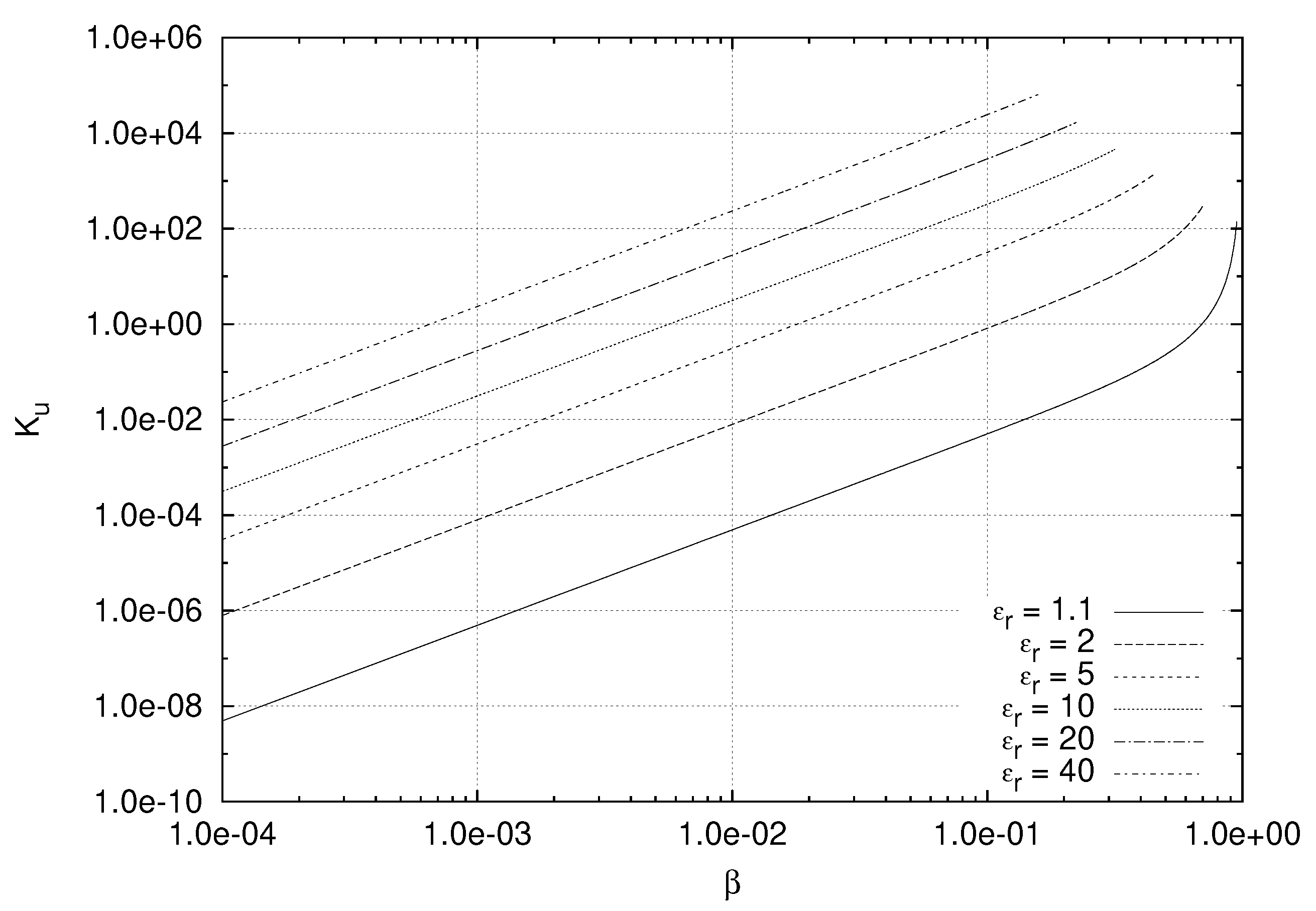
. We get
In
Figure 1,
is plotted with respect to
, with
as a parameter. It shows that the range
of
for which the validity of condition (
9) is guaranteed becomes larger and larger as
gets smaller and smaller, as expected. However, our analysis provides quantitative results on such a range. As it is easy to check, it is so large that no significant restriction on
emerges for practical applications.
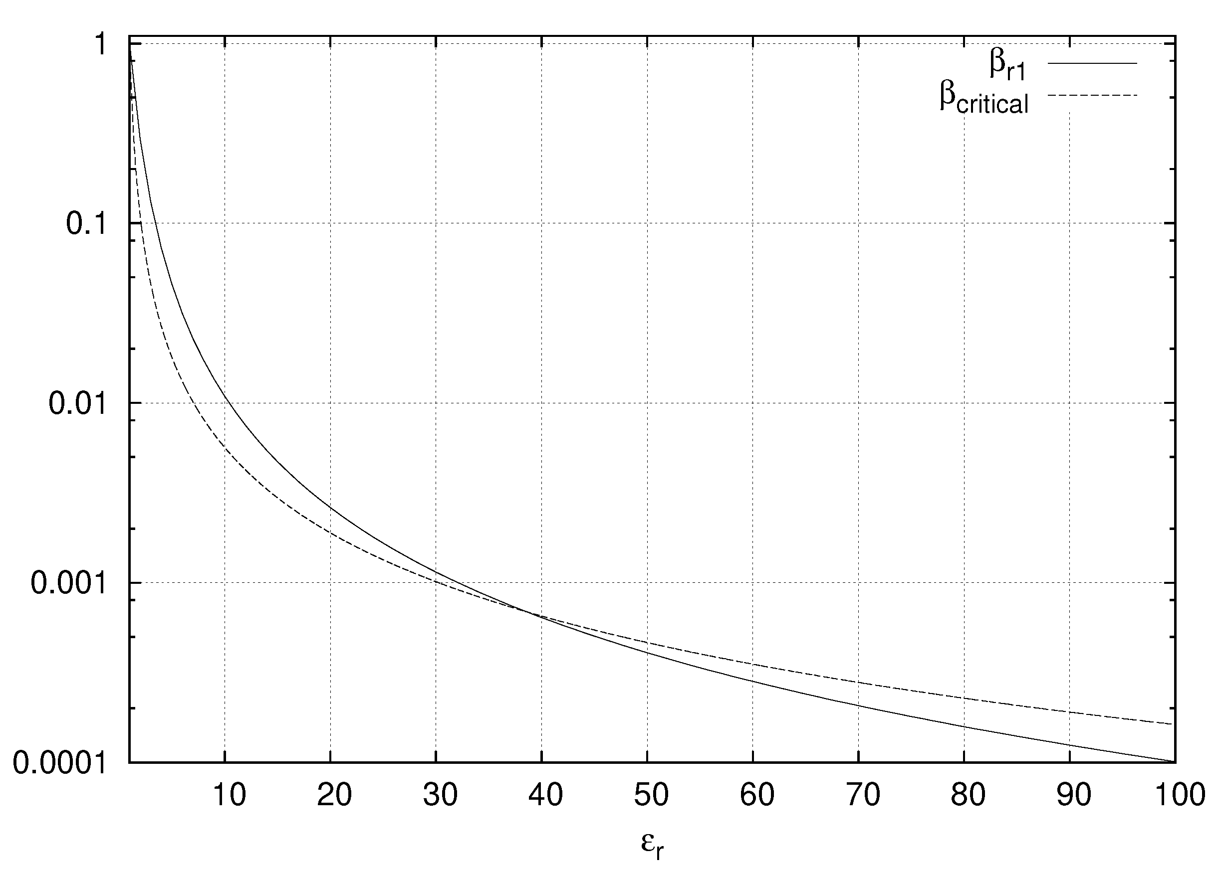
The plot of
is shown, together with another significant threshold value obtained in the next subsection, in
Figure 2.
7.2. Checking Conditions (10) for Problems Involving Rotating Objects
In this section, we examine the situations in which condition (
10) holds true for the class of problems considered. By definition, inside and outside the scatterer, we get
,
,
,
. In order to check the indicated condition, we need to find the constants
,
,
and
. As for
and
, by using Equations (
32) and (
33), we have to evaluate the suprema involved just inside the scatterer. Since
, we can focus just on one of the two constants. The eigenvalues of
are found to be 0 and
(with multiplicity 2). As already pointed out, in the following, in order to simplify the analysis, we assume that the scatterer medium is characterized by
and
in its rest frame. Under this hypothesis, the field
is strictly positive and then
We already know that inside the scatterer the eigenvalues of
are
and
while outside it we have
. Under the indicated hypotheses for the scatterer medium, since
, from Lemma 1 (see Equation (
26)), we trivially get that HM13 is satisfied with
Similarly, the eigenvalues of
inside the scatterer are
and
while outside the rotating object we have
. Since
by Equation (
29), we obtain
which is positive when
. Under this condition, HM14 is satisfied as well.
By using Equations (
74)–(
76), the crucial inequality which is present in assumption HM15 reads
After the substitution of
and
, it can be shown to be equivalent to the following:
The left-hand side in inequality (
78) is a parabola in terms of
. We can find two roots
,
given by
which are both real numbers. Such numbers are positive because the parabola becomes larger and larger for
and is equal to 1 and has a negative derivative (equal to
) when
.
In particular, we have that
since
and
because
.
Since a value greater than one is not possible for
, condition HM15 can only be satisfied for
in the range
. In the same range of
condition, HM14 is a priori satisfied (see Equation (
80) and the comment after Equation (
76)) and then (
10) does hold true.
The behaviours of
and
versus
are shown in
Figure 2. In order to satisfy conditions (
9) and (
10) and then to obtain the well posedness of the problem,
should be smaller than the smallest of
and
. The two plots in
Figure 2 cross at about
and for smaller (respectively, larger) values the stronger condition on
is given by condition (
9) (respectively, (
10)).
7.3. Application to Rotating Sphere
In this subsection, we apply the theory to a specific case: a rotating sphere of radius
is illuminated by a linearly polarized plane wave propagating along the
x-axis. A first order approximation of the solution of this problem is given by the semi-analytic procedure discussed by De Zutter in [
1].
Our formulation of the problem requires the definition of a bounded domain , which is taken as a sphere of radius . The boundary conditions we enforce on have Y equal to the admittance of vacuum and are inhomogeneous (), to take account of the incident field.
The parameters considered are , , m, m. The incident plane wave has a frequency of 50 MHz and an amplitude of the electric field of 1 V/m.
In order to analyze significant test cases for our theory and, at the same time, show its generality, we consider exceptionally large rotational speeds, without worrying about the mechanical stability of the rigid body. The rotating speed we consider is
rad/s, which corresponds to a maximum normalized velocity of
. This is within the limits of applicability of our theory since for
we get
and
. The above qualitative considerations, which apply also to the next test case (see
Section 7.4), justify the simplified approach we have adopted (see Remark 1).
A comparison of the first order edge element based Galerkin finite element solution against the De Zutter semi-analytic procedure is carried out when the incident field is polarized along the z-axis and the spherical domain is discretized rather uniformly with a mesh having 475,797 nodes and 2,496,192 tetrahedra.
All values of the significant quantities defining our model are reported in
Table 1. It includes also the parameters defining the model considered in the next subsection.
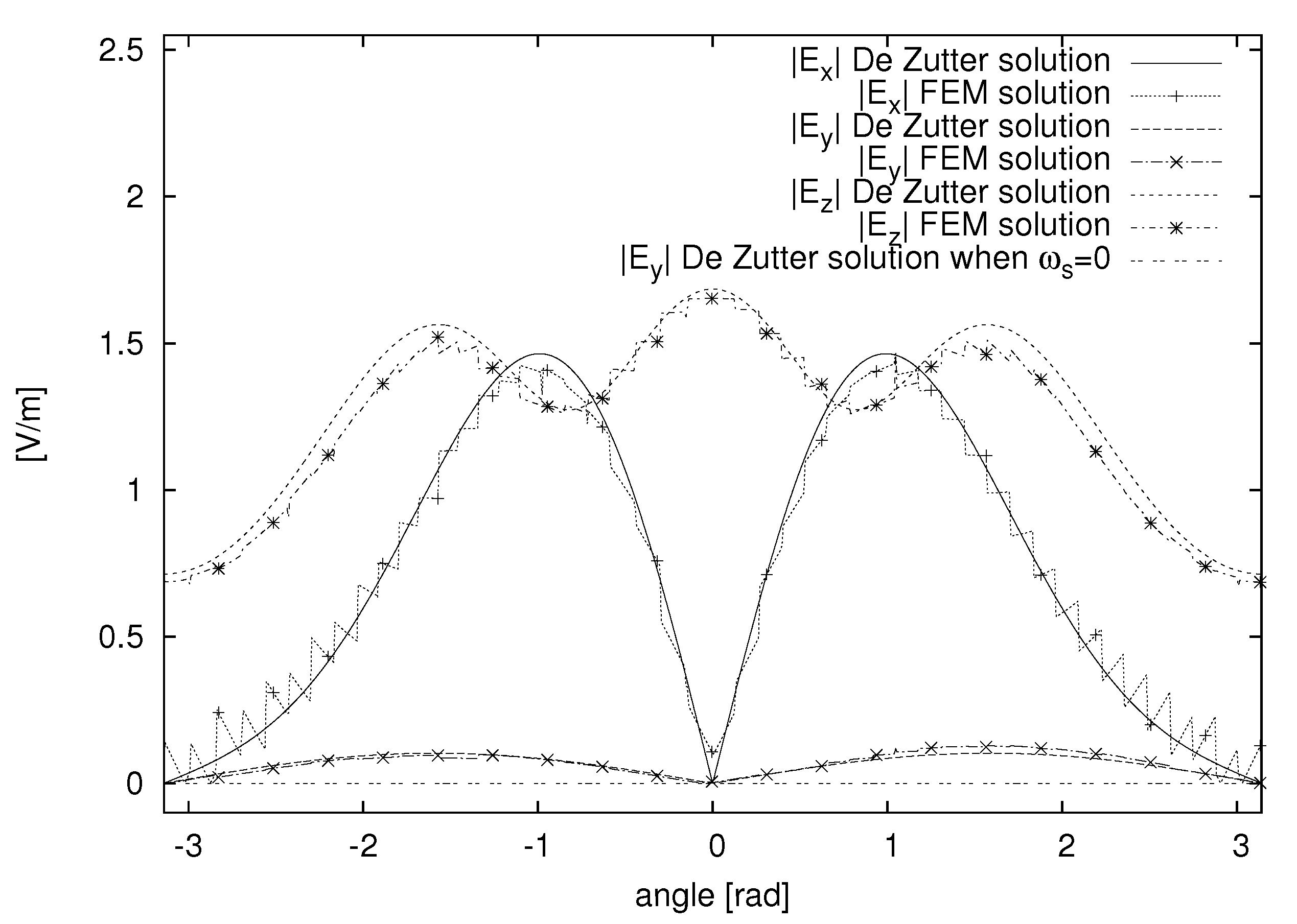
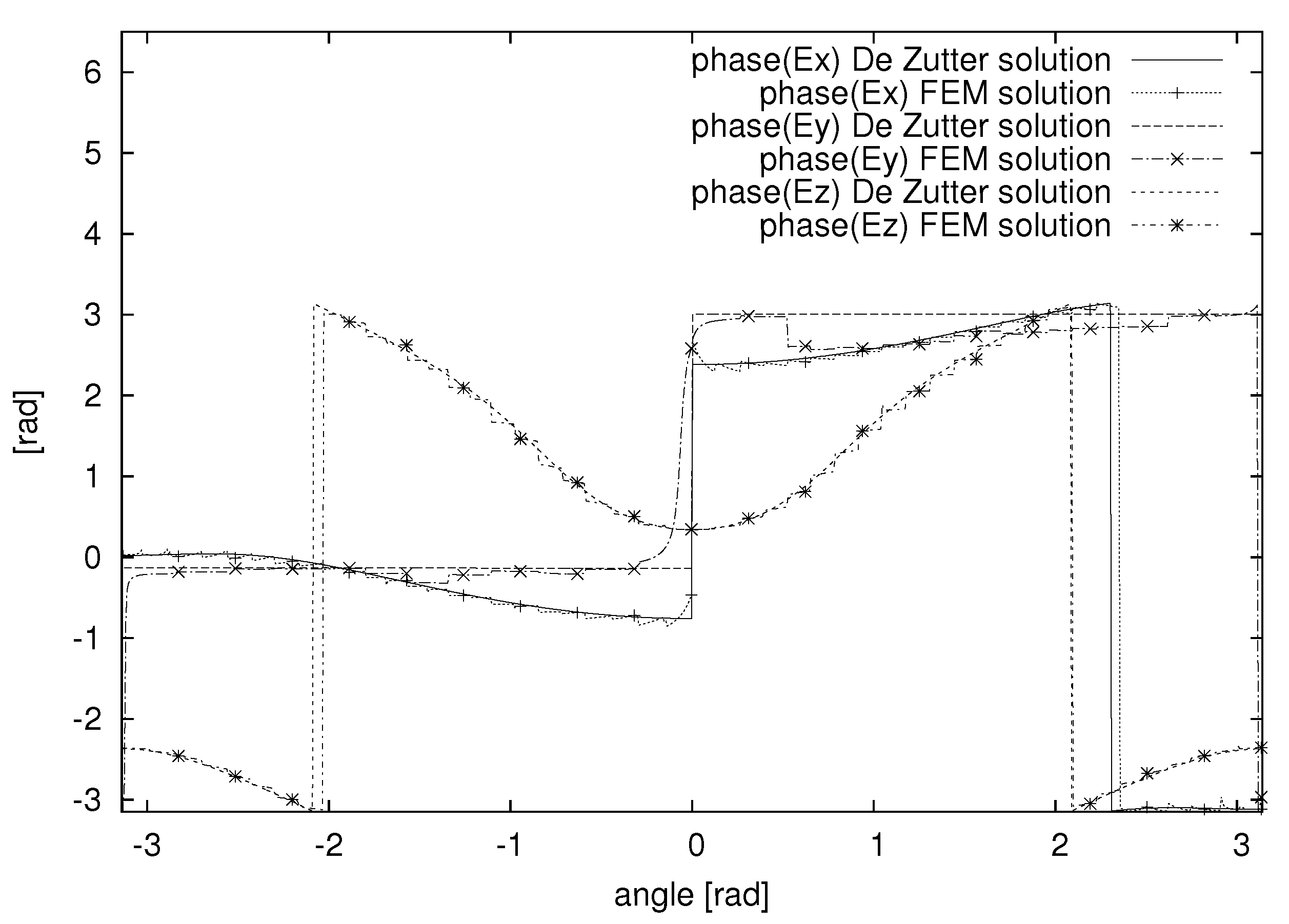
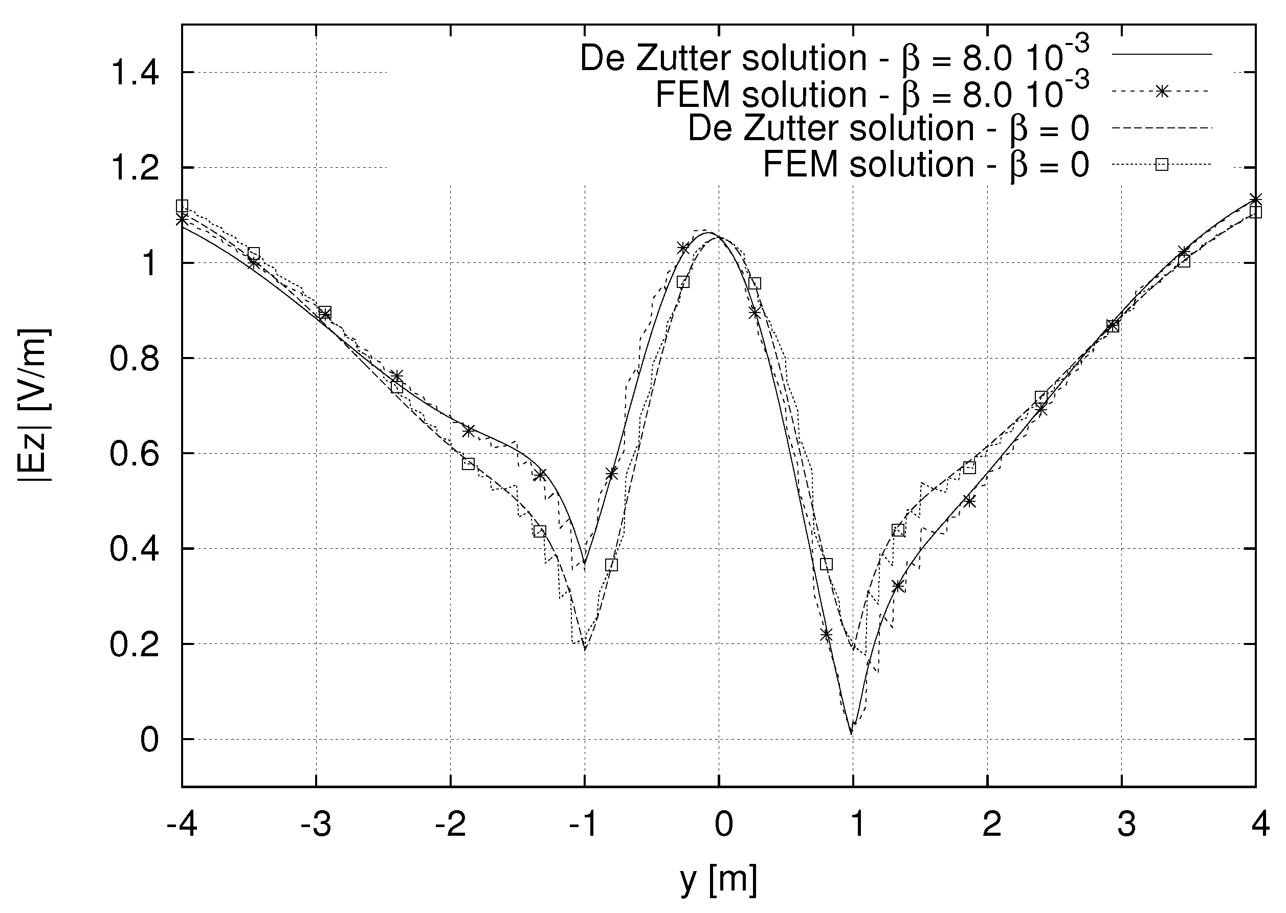
Figure 3 and
Figure 4 show, respectively, the magnitude and phase of the components of the electric field evaluated along a circle in the
plane, which is centered at the origin and has a radius of 1.5 m. The results obtained from the finite element solver are compared with the semi-analytical solution obtained using the De Zutter procedure [
1]. All three components are in very good agreement. Due to the well posedness and the finite element approximability of the problem, this shows that the De Zutter first order (in
) approximation provides reliable results even for very large rotational speeds.
In particular, we can observe that the
y-component of the field is purely a result of rotation. This component amounts to 10 percent of the incident field. These kinds of effects on the fields can be particularly important for inverse problems to figure out the rotational speeds, for example, by extending the algorithms discussed in [
37,
38].
The same sort of agreement between the two solutions is further confirmed by the fields along similar circles on other planes or along lines parallel to coordinate axes, for different polarizations and directions of propagation of the illuminating field.
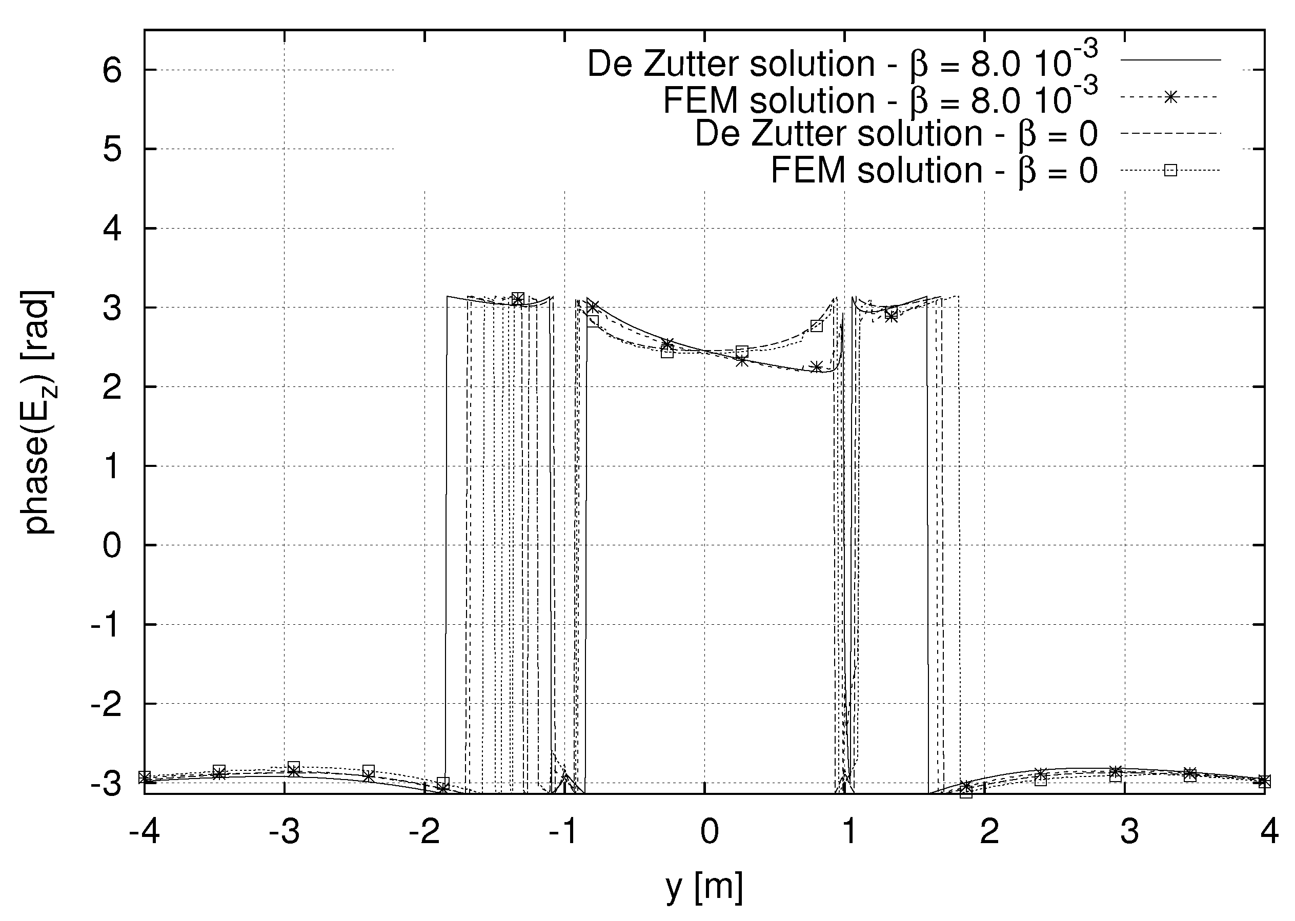
For example,
Figure 5 and
Figure 6 show the magnitude and phase of the z component of electric field along the
y-axis. Along this line, the motion of the sphere causes a difference in magnitude of up to 20 percent of the incident field.
7.4. Application to Rotating Torus
Thus far, we have considered problems for which a semi-analytic solution is available. In order to illustrate the full relevance of the new results, we now tackle problems for which no solution can be found in the open literature, to the best of the authors’ knowledge.
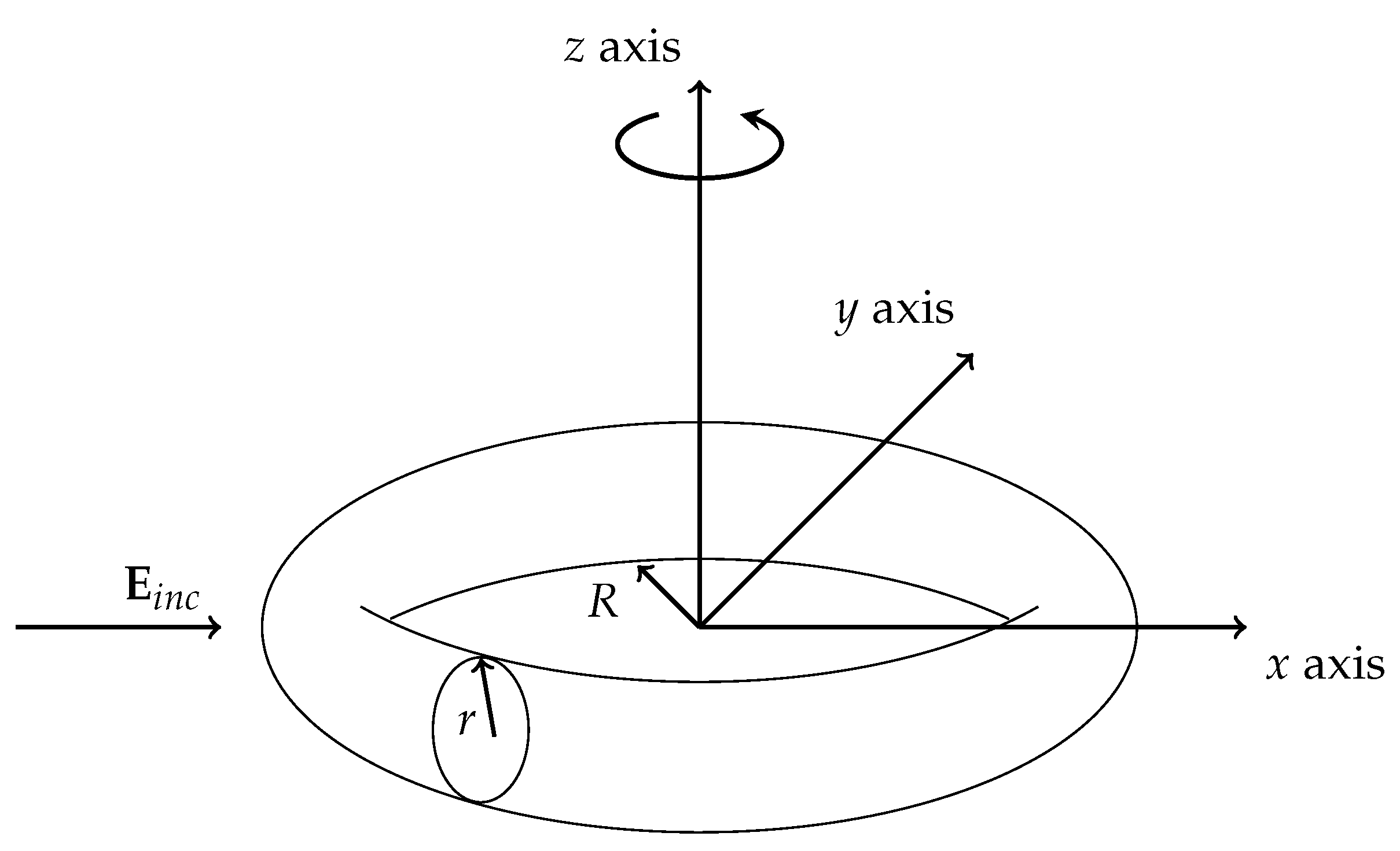
For this, let us consider a homogeneous torus rotating about its axis. The geometry of the problem is described in
Figure 7.
The value of both radii (R and r) is 0.15 m. The torus is made of a material with . The domain of numerical investigation is a sphere of radius 2 m. We consider a plane wave incident along the x-axis with the electric field polarized along the z-axis and with magnitude 1 V/m and frequency MHz. For , the upper bounds for allowing the application of our theory are given by and . Respecting these limits lets us consider values of rad/s, which corresponds to a maximum value of .
The first order edge element based Galerkin finite element solution we show in the following is obtained with a three-dimensional tetrahedral mesh having 2,192,940 elements and 36,993 nodes.
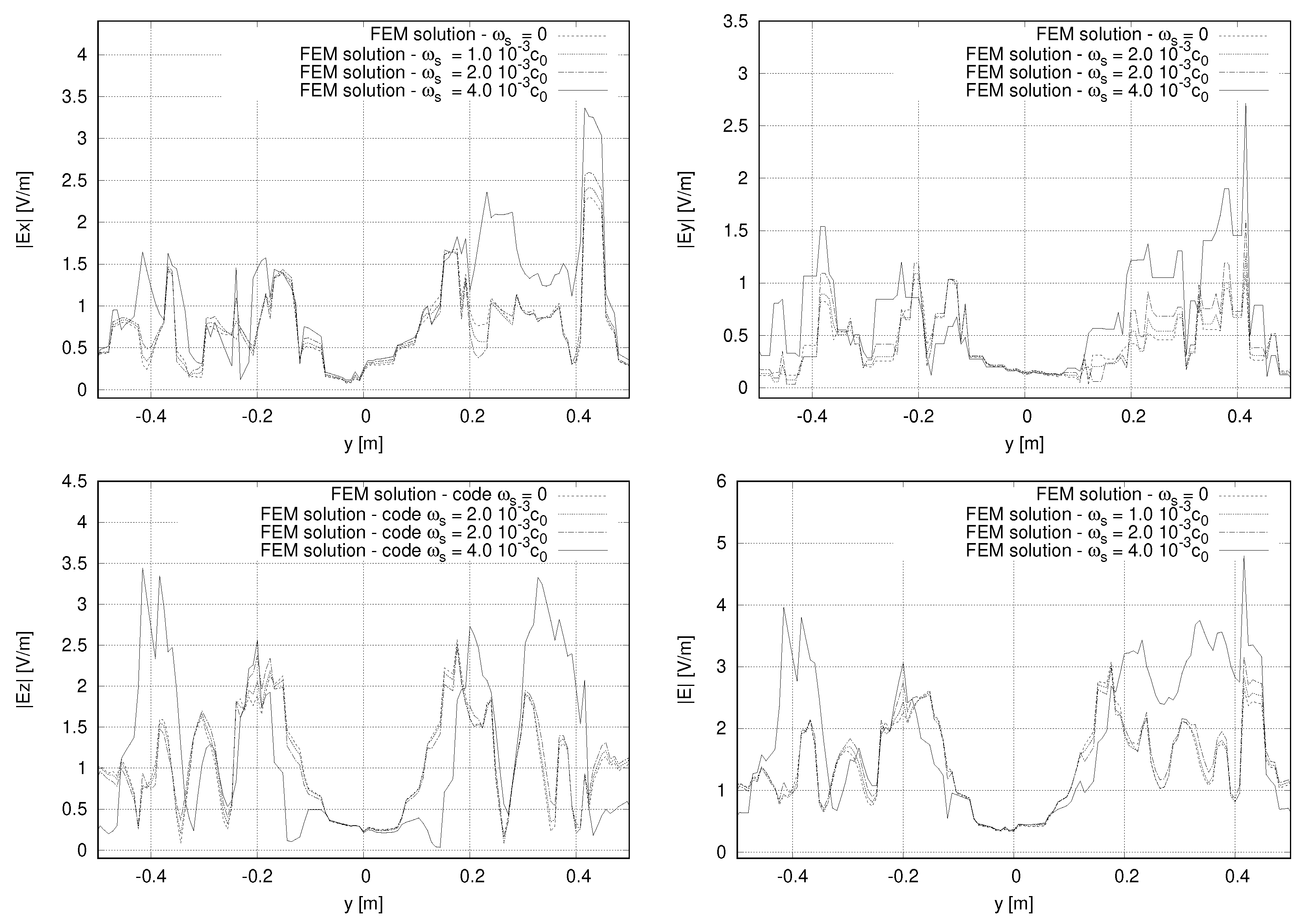
To gain an understanding of the solution, we may consider the behaviours of the field along the three coordinate directions for different rotating speed values. Here, we consider
in the set
. The electric field components along the
x-axis are shown in
Figure 8.
In this case, the largest effect due to motion occurs in the z component of the field, where a difference as large as twice the incident field can be observed between the cases with
and
. For the other two speeds considered, the effects are smaller but still discernible. There are effects also on the components
and
along the
x-axis, the maximum difference from the stationary solution being around twice the incident field in the former case and fifty percent of the incident field in the latter one. The norm of the total field
is dominated by the z-component and hence both of them carry roughly the same information when plotted along the
x-axis. Along the
y-axis for
, the differences from the stationary case are as large as twice the incident field for
, fifty percent of incident field for
and three times for
. This is shown in
Figure 9.
In this case, the total field is also largely similar to the z component and the difference from the stationary solution is about three times the incident field. For the other speeds considered, the rotational effects on the fields are quite small along this direction. Finally, we do not show the behaviour of the electric field along the z-axis because, in this case, the effects due to motion for all the components are quite small (less than 2 percent) for the speeds considered.
Hence, we can conclude that in this case the fields along x- and y -directions carry significant information about the rotating speed of the toroidal scatterer.
As previously mentioned, the changes in the fields induced by the motion are important because it may be useful for the reconstruction of the velocity profiles of rotating objects. This could be of interest, for example, for rotating celestial bodies. Moreover, since our theory guarantees the well posedness of the problems and the convergence of the numerical solutions, the presented results can be considered as benchmarks for other approaches or numerical techniques.


