A New Filter Nonmonotone Adaptive Trust Region Method for Unconstrained Optimization

Abstract

In this paper, a new filter nonmonotone adaptive trust region with fixed step length for unconstrained optimization is proposed. The trust region radius adopts a new adaptive strategy to overcome additional computational costs at each iteration. A new nonmonotone trust region ratio is introduced. When a trial step is not successful, a multidimensional filter is employed to increase the possibility of the trial step being accepted. If the trial step is still not accepted by the filter set, it is possible to find a new iteration point along the trial step and the step length is computed by a fixed formula. The positive definite symmetric matrix of the approximate Hessian matrix is updated using the MBFGS method. The global convergence and superlinear convergence of the proposed algorithm is proven by some classical assumptions. The efficiency of the algorithm is tested by numerical results.

1. Introduction

Consider the following unconstrained optimization problem:

$$\underset{x\in R^n}{\min }f(x),$$

(1)

where $f$:$R^n\to R$ is a twice continuously differentiable function. The trust region method is one of the prominent classes of iterative methods. At the iteration point $x_k$, the trial step $d_k$ is obtained by the following quadratic subproblem:

$$\underset{d\in R^n}{\min }{m}_k(d)=g_k^{T}d+\frac{1}{2}{d}^T{B}_{k}d,$$

(2)

$$\Vert d\Vert \le {\Delta }_k$$

where $\Vert .\Vert$ is the Euclidean norm, $f_k=f(x_k)$, $g_k=\nabla f(x_k)$, $G_k={\nabla }^{2}f(x_k)$, $B_k$ is a symmetric approximation of $G_k$, and ${\Delta }_k$ is a trust region radius. The most ordinary ratio is defined as follows:

$${\rho }_k=\frac{f_k-f(x_k+d)}{m_k(0)-m_k(d_k)},$$

(3)

Generally, the numerator is referred to as the actual reduction and the denominator is known as the predicted reduction.

The disadvantage of the traditional trust region method is that the subproblem needs to be solved many times to achieve an acceptable trial step in one iteration. To overcome this drawback, Mo et al. [1] first proposed a nonmonotone trust region algorithm with a fixed step length. When the trial step is not acceptable, we use a fixed step length to find a new iteration point instead of resolving the subproblem. Based on this advantage, Ou, Hang, and Wang have proposed a trust region algorithm with fixed step length in [2,3,4], respectively. The fixed step length is computed by

$${\alpha }_k=-\frac{\delta g_k^T{d}_k}{d_k^T{B}_k{d}_k},$$

(4)

It is well known that the strategy of selecting a trust region radius has a significant impact on the performance of the trust region methods. In 1997, Sartenaer [5] presented a strategy which can automatically determine an initial trust region radius. This fact leads to an increase in the number of subproblems to be solved in some problems, thereby reducing the efficiency of these methods. In 2002, Zhang et al. [6] provided another scheme to reduce the number of subproblems that need to be solved, where the trust region radius uses: ${\Delta }_k=c^p\Vert g_k\Vert \Vert {\widehat{B}}_k^{-1}\Vert$, ${\widehat{B}}_k=B_k+iI$, where $i\in N$. Zhang’s strategy requires an estimation of the inverse of the matrixes $B_k$ and ${\widehat{B}}_k^{-1}$ in each iteration; however, Li [4] has suggested another practically efficient adaptive trust region radius that uses ${\Delta }_k=\frac{\Vert d_{k-1}\Vert }{\Vert y_{k-1}\Vert }\Vert g_k\Vert$. The strategy requires not only the gradient value but also the function value. Inspired by these facts, some modified versions of adaptive trust region methods have been proposed in [7,8,9,10].

As we all know, monotone techniques may slow down the rate of convergence, especially in the presence of the narrow curved valley. The monotone techniques require the value of the function to be decreased at each iteration. In order to overcome these disadvantages, Deng et al. [11] proposed a nonmonotone trust region algorithm in 1993. The general nonmonotone term $f_{l(k)}$ is defined by

$$f_{l(k)}=f(x_{l(k)})=\underset{0\le j\le m(k)}{\max }\{f_{k-j}\}k=0,1,2,\dots ,$$

(5)

where $m(0)=0$, $0\le m(k)\le \min \{N,m(k-1)+1\}$, and $N\ge 0$ is an integer. Deng et al. [11] modified the ratio (3) which evaluates the consistency between the quadratic model and the objective function in trust region methods. The most common nonmonotone ratio is defined as follows:

$${\tilde{\rho }}_k=\frac{f_{l(k)}-f(x_k+d_k)}{m_k(0)-m_k(d_k)}$$

(6)

The general nonmonotone term $f_{l(k)}$ suffers from various drawbacks, such as the fact that numerical performance is highly dependent on the choice of $N$. In order to introduce a more suitable nonmonotone strategy, Ahookhosh et al. [12] proposed a new nonmonotone ratio as follows.

$${\widehat{\rho }}_k=\frac{R_k-f(x_k+d_k)}{m_k(0)-m_k(d_k)},$$

(7)

where

$$R_k={\eta }_k{f}_{l(k)}+(1-{\eta }_k)f_k,$$

(8)

in which ${\eta }_k\in [{\eta }_{\min },{\eta }_{\max }]$, with ${\eta }_{\min }\in [0,1)$, and ${\eta }_{\max }\in [{\eta }_{\min },1]$. We recommend that interested readers refer to [13,14] for more details and progress on the nonmonotone trust region algorithm.

In order to overcome the difficulties associated with using the penalty function, especially the adjustment of the penalty parameter. The filter methods were recently presented by Fletcher and Leyffer [15] for constrained nonlinear optimization. More recently, Gould et al. [16] explored a new nonmonotone trust region algorithm for the unconstrained optimization problems with the multidimensional filter technique in [17]. Compared with the standard nonmonotone algorithm, the new algorithm dynamically determines iterations based on filter elements and increases the possibility of the trial step being accepted. Therefore, this topic has received great attention in recent years (see [18,19,20,21]).

The remainder of this paper is organized as follows. In Section 2, we describe a new trust region method. The global convergence is investigated in Section 3. In Section 4, we prove the superlinear convergence of the algorithm. Numerical results are shown in Section 5. Finally, the paper ends with some conclusions in Section 6.

2. The New Algorithm

In this section, we propose a trust region method by combining a new trust region radius and the modified trust region ratio to effectively solve unconstrained optimization problems. In each iteration, a trial step $d_k$ is generated by solving an adaptive trust region subproblem,

$$\underset{d\in {ℝ}^n}{\min }{m}_k(d)=g_k^{T}d+\frac{1}{2}{d}^T{B}_{k}d,$$

(9)

$$\Vert d\Vert \le {\Delta }_k:=c_k{\Vert g_k\Vert }^{\gamma },$$

(10)

where $0<\gamma <1$ and $c_k$ is an adjustment parameter. Prompted by the adaptive technique, the proposed method has the following effective properties: it is not necessary to calculate the matrix of the inverse and the value of each iteration point, and the algorithm also reduces the related workload and calculation time.

In fact, the matrix $B_k$ is usually obtained by approximation, and the subproblems are only solved roughly. In this case, it may be more reasonable to adjust the next trust radius ${\Delta }_{k+1}$, not only according to ${\widehat{\rho }}_k$, but also by considering the use of $\left\{{\widehat{\rho }}_{k-m},\dots ,{\widehat{\rho }}_k\right\}$. To improve the efficiency of the nonmonotone trust region methods, we can define the modified ratio formula based on (7) as follows:

$${\widehat{\rho }}^{\prime }{}_k={\displaystyle \sum _{i=1}^{\min \{k,m\}}{w}_{ki}}{\widehat{\rho }}_{k-i+1},$$

(11)

where $m$ is a positive integer and $w_{ki}$ is the weight of ${\widehat{\rho }}_{k-i+1}$, such that ${\displaystyle \sum _{i=1}^{\min \{k,m\}}{w}_{ki}}=1$.

More exactly, ${\widehat{\rho }}_k$ can be used to determine whether the trial step is acceptable. Adjusting the next radius ${\Delta }_{k+1}$ depends on (11), thus $c_k$ is updated by

$$c_{k+1}=\{\begin{array}{ll}\min \{{\beta }_2{c}_k,c_{\max }\}& \mathrm{if}{\widehat{\rho }}_k{}^{\prime }\ge {\mu }_2\\ c_k& \mathrm{if}{\mu }_1\le {\widehat{\rho }}_k{}^{\prime }<{\mu }_2\\ {\beta }_1{c}_k& \mathrm{if}{\widehat{\rho }}_k{}^{\prime }<{\mu }_1\end{array},$$

(12)

In what follows, we refer to $\nabla f(x_k)$ by $g_k=g(x_k)$. When an $i-\mathrm{th}$ component of $g_k$ is needed, we denote it using $g_i(x_k)$. Based on this filter, we say that an iterate point $x_1$ dominates $x_2$ if, and only if

$$\left|g_i\left(x_1\right)\right|\le \left|g_i\left(x_2\right)\right|\hspace{1em}\forall i=1,2,\dots ,n.$$

(13)

A multidimensional filter $F$ is a list of $n$-tuples of the form $\left(g_1\left(x_k\right),g_2\left(x_k\right),\dots ,g_n\left(x_k\right)\right)$, such that

$$\left|g_j\left(x_k\right)\right|\le \left|g_j\left(x_l\right)\right|\hspace{1em}\hspace{1em}j\in \left\{1,2,3,\dots ,n\right\},$$

(14)

where $g_k$, $g_l$ belong to $F$.

For all $g\left(x_l\right)\in F$, a new trial point is acceptable if there exists $j\in \left\{1,2,3,\dots ,n\right\}$, such that

$$\left|g_j(x_k)\right|\le \left|g_j(x_l)\right|-{\gamma }_g\Vert g(x_l)\Vert \hspace{1em}\hspace{1em}{\gamma }_g\in (0,\frac{1}{\sqrt{n}}),$$

(15)

If the iterate point $x_k^{+}$ is acceptable, we add $g\left(x_k^{+}\right)$ to the filter. Meanwhile, we remove all the points which are dominated by $x_k^{+}$ from the filter. In the general filter trust region algorithm, for the trial point $x_k^{+}$ satisfying ${\widehat{\rho }}_k<{\mu }_1$, we verify whether it is accepted by filter $F$. In our algorithm, it is the trial point $x_k^{+}$ that satisfies $0<{\widehat{\rho }}_k<{\mu }_1$, and verifies whether or not it is accepted by the filter $F$.

Our discussion can be summarized as the following Algorithm 1.

Algorithm 1. A new filter nonmonotone adaptive trust region method.

Step 0. (Initialization) An initial point $x_0\in R^n$ and a symmetric matrix $B_0\in R^n\times R^n$ are given. The constants $0<{\mu }_1<{\mu }_2<1$, $0<{\eta }_{\min }\le {\eta }_{\max }<1$, $\tau >0$, $N>0$, $\epsilon >0$, ${\eta }_{\min }\in [0,1)$ and ${\eta }_{\max }\in [{\eta }_{\min },1)$ are also given. Step 1. If $\Vert g_k\Vert \le \epsilon$, then stop. Step 2. Solve the subproblem (2) to find the trial step $d_k$. Step 3. Choose $w_{ki}\in \left[0,1\right]$, which satisfies ${\displaystyle \sum _{i=1}^{\min \{k,m\}}{w}_{ki}}=1$. Compute $R_k$, ${\widehat{\rho }}_k$, and ${\widehat{\rho }}_k{}^{\prime }$, respectively. Step 4. Test the trial step. If ${\widehat{\rho }}_k\ge {\mu }_1$, then set $x_{k+1}=x_k^{+}$. Otherwise compute $g_k^{+}=\nabla f(x_k^{+})$;   if $x_k^{+}$ is acceptable by the filter $F$, then $x_{k+1}=x_k^{+}$, add $g_k^{+}=\nabla f(x_k^{+})$ into the filter $F$.   Otherwise, find the step length ${\alpha }_k$ satisfying (4), set $x_{k+1}=x_k+{\alpha }_k{d}_k$.   end(if) end(If) Step 5. Update the trust region radius by ${\Delta }_{k+1}=c_{k+1}{\Vert g_{k+1}\Vert }^{\gamma }$, where $c_{k+1}$ is updated by (12). Step 6. Compute the new Hessian approximation $B_{k+1}$ by a modified BFGS method formula. Set $k=k+1$, and return to Step 1.

In order to obtain convergence results, we use the following notation:

$D=\left\{k|{\widehat{\rho }}_k\ge {\mu }_1\right\}$, $A=\left\{k|0<{\widehat{\rho }}_k<{\mu }_1\mathrm{and}{x}_k^{+}\mathrm{is}\mathrm{accepted}\mathrm{by}\mathrm{the}\mathrm{filter}F\right\}$, $S=\left\{k|x_{k+1}=x_k+d_k\right\}$. Then, we have $S=\left\{k|{\widehat{\rho }}_k\ge {\mu }_1\mathrm{or}{x}_k^{+}\mathrm{is}\mathrm{accepted}\mathrm{by}\mathrm{the}\mathrm{filter}F\right\}$. When $k\notin S$, we have $x_{k+1}=x_k+{\alpha }_k{d}_k$.

3. Convergence Analysis

To establish the convergence of Algorithm 1, we make the following common assumption.

Assumption 1.

H1.The level set$L(x_0)=\{x\in R^n|f(x)\le f(x_0)\}\subset \mathsf{\Omega }$,where$\mathsf{\Omega }\in R^n$is bounded$f(x)$is continuously differentiable on the level set$L(x_0)$.

H2. The matrix$B_k$is uniformly bounded, i.e., there exists a constant$M_1>0$such that$\Vert B_k\Vert \le M_1$.

H3. There exists constant$v$such that$v{\Vert d\Vert }^2\le d^T{B}_{k}d$, for all$k\in N\cup \left\{0\right\}$.

Remark 1.

In order to analyze the convergence of the new algorithm, it should be seen to that the trial step$d_k$satisfies the following conditions:

$$m_k(0)-m_k(d_k)\ge \tau \Vert g_k\Vert \min \left\{{\Delta }_k,\frac{\Vert g_k\Vert }{\Vert B_k\Vert }\right\},$$

(16)

$$g_k^T{d}_k\le -\tau \Vert g_k\Vert \min \left\{{\Delta }_k,\frac{\Vert g_k\Vert }{\Vert B_k\Vert }\right\},$$

(17)

where the constant$\tau \in (0,1)$.

Remark 2.

If$f$is a twice continuously differentiable function, then H1 means that there is a positive constant$L$such that

$$\Vert \nabla f(x)-\nabla f(y)\Vert \le L\Vert x-y\Vert \forall x,y\in \mathsf{\Omega },$$

(18)

Lemma 1.

For all$k$, we can obtain that

$$\left|f_k-f\left(x_k+d_k\right)-\left(m_k\left(0\right)-m_k\left(d_k\right)\right)\right|\le O\left({\Vert d_k\Vert }^2\right),$$

(19)

Proof. 

The proof is given by using Taylor’s expansion and H3. □

Lemma 2.

Suppose that H1-H3 hold, the sequence$\left\{x_k\right\}$is generated by Algorithm 1. Moreover, assume that there exists a constant$0<\epsilon <1$such that$\Vert g_k\Vert >\epsilon$, for all$k$. Then, for every$k$, there exists a nonnegative integer$p$, so that$x_{k+p+1}$is a successful iteration point, i.e.,${\widehat{\rho }}_{k+p}\ge {\mu }_1$.

Proof. 

We are able to prove this by using contradiction; we assume that there exists an iteration $k$, and that $x_{k+p+1}$ is an unsuccessful iteration point for all nonnegative integer $p$, i.e.,

$${\widehat{\rho }}_{k+p}<{\mu }_{1}p=0,1,2,\dots .$$

(20)

It follows from (11) that ${\widehat{\rho }}_{k+p}{}^{\prime }<{\mu }_{1}p=0,1,2,\dots$. Thus, using (10) and (12), we show

$${\Delta }_{k+p+1}\le {\beta }_1^{p+1}{c}_k{\Vert {\mathrm{g}}_{k+p}\Vert }^{\gamma }\le {\beta }_1^{p+1}{c}_{\max }{\Vert {\mathrm{g}}_k\Vert }^{\gamma }.$$

(21)

As a matter of fact, in the unsuccessful iterations, we have $x_{k+p}=x_k$. Thus, according to $0<{\beta }_1<1$ and (21), we have

$$\underset{p\to \infty }{\lim }{\Delta }_{k+p+1}=0.$$

(22)

Now, using Lemma 1 and (16) we get

$$\begin{array}{ll}\left|\frac{f\left(x_{k+p}\right)-f\left(x_{k+p}+d_{k+p}\right)}{m_{k+p}(0)-m_{k+p}(d_{k+p})}-1\right|& =\left|\frac{f\left(x_{k+p}\right)-f\left(x_{k+p}+d_{k+p}\right)-\left(m_{k+p}(0)-m_{k+p}(d_{k+p})\right)}{m_{k+p}(0)-m_{k+p}(d_{k+p})}\right|\\ & \le \frac{O\left({\Vert d_{k+p}\Vert }^2\right)}{\tau \Vert g_{k+p}\Vert \min \left\{{\Delta }_{k+p},\frac{\Vert g_{k+p}\Vert }{\Vert B_{k+p}\Vert }\right\}}\\ & \le \frac{O\left({\Vert d_{k+p}\Vert }^2\right)}{\tau \epsilon \min \left\{{\Delta }_{k+p},\frac{\epsilon }{M_1}\right\}}\\ & \le \frac{O\left({\Delta }_{k+p}{}^2\right)}{O\left({\Delta }_{k+p}\right)}\to 0\left(p\to \infty \right)\end{array}$$

According to the definition of $R_k$, we get $R_k\ge {\eta }_k{f}_k+(1-{\eta }_k)f_k=f_k$. Thus, for sufficiently large $p$ we have,

$${\widehat{\rho }}_{k+p}=\frac{R_{k+p}-f(x_{k+p}+d_{k+p})}{m_{k+p}(0)-m_{k+p}(d_{k+p})}\ge \frac{f_{k+p}-f(x_{k+p}+d_{k+p})}{m_{k+p}(0)-m_{k+p}(d_{k+p})}\to 1,$$

(23)

which contradicts (20). This completes the proof of Lemma 2. □

Lemma 3.

Suppose that H1–H3 hold and the sequence$\left\{x_k\right\}$is generated by Algorithm 1. Set$\delta \in \left(0,\min \left\{1,\frac{v}{L}\right\}\right)$. For$k\notin S$, we have

$$f_{k+1}-R_k\le \frac{\delta }{2}\left(1-\frac{L\delta }{v}\right)g_k^T{d}_k\le 0,$$

(24)

Proof. 

According to the definition of $R_k$, for all $k$, we have $f_k\le R_k$. Using the differential mean value theorem, we get

$$f_{k+1}-R_k\le f_{k+1}-f_k=g{(\xi )}^T(x_{k+1}-x_k),$$

(25)

where $\xi \in [x_k,x_{k+1}]$. For $k\notin S$ and (18), we obtain

$$\begin{array}{ll}g{(\xi )}^T(x_{k+1}-x_k)& =g_k^T(x_{k+1}-x_k)+(g(\xi )-g_k{)}^T(x_{k+1}-x_k)\\ & \le g_k^T(x_{k+1}-x_k)+\Vert g(\xi )-g_k\Vert \Vert x_{k+1}-x_k\Vert \\ & \le g_k^T(x_{k+1}-x_k)+L{\Vert x_{k+1}-x_k\Vert }^2\\ & =g_k^T{\alpha }_k{d}_k+L{\alpha }_k{}^2{\Vert d_k\Vert }^2\\ & =(1-L\delta {\Vert d_k\Vert }^2/d_k^T{B}_k{d}_k){\alpha }_k{g}_k^T{d}_k\\ & \le (1-L\delta /v){\alpha }_k{g}_k^T{d}_k\end{array}$$

(26)

Note that (4) and (16) imply that ${\alpha }_k\ge \frac{\delta }{2}$ for all. Setting $\delta \in \left(0,\min \left\{1,\frac{v}{L}\right\}\right)$ means that $1-L\delta /v>0$. According to (17), (25), and (26), we can conclude that (24) holds. □

Lemma 4.

Suppose that the sequence$\left\{x_k\right\}$is generated by Algorithm 1. Then, we have$\left\{x_k\right\}\subset L(x_0)$.

Proof. 

We can proceed by induction. When $k=0$, apparently $x_0\in L(x_0)$.

Assuming that $x_k\in L(x_0)$$(k\ge 0)$ holds, we would obtain $f_k\le f_0$. Then, we can prove that $x_{k+1}\in L(x_0)$.

(a) When $k\in S$, consider two cases:

Case 1: $k\in D$. According to (7) and (16), we obtain $R_k-f_{k+1}\ge {\mu }_1(m_k(0)-m_k(d_k))\ge 0$. Thus, we have $R_k\ge f_{k+1}$. Following the definition of $R_k$ and $f_{l(k)}$, we obtain

$$R_k={\eta }_k{f}_{l(k)}+(1-{\eta }_k)f_k\le {\eta }_k{f}_{l(k)}+(1-{\eta }_k)f_{l(k)}=f_{l(k)}.$$

(27)

The above two inequalities show that

$$f_{k+1}\le R_k\le f_{l(k)}\le f_0.$$

(28)

Case 2: $k\in A$. According to $0<{\widehat{\rho }}_k<{\mu }_1$, we have $R_k-f(x_k+d_k)>0$. Thus, we get $f_{k+1}\le R_k\le f_{l(k)}\le f_0$.

(b) When $k\notin S$. Using Lemma 3 and (27), we obtain $f_{k+1}\le R_k\le f_{l(k)}\le f_0$.

Now, we can conclude that $\left\{x_k\right\}\subset L\left(x_0\right)$. □

Lemma 5.

Suppose that H1–H3 hold, and the sequence$\left\{x_k\right\}$is generated by Algorithm 1. This would mean that$\left\{f_{l\left(k\right)}\right\}$is a not a monotonically increasing sequence, nor is it convergent.

Proof. 

Now, we can prove that the sequence $\left\{f_{l\left(k\right)}\right\}$ is not a monotonically increasing sequence. Thus, we consider two cases:

Case 1: For $k<N$, it is clear that $m(k)=k$. Since, for any $k$, we have $f_k\le f_0$. Thus, we get $f_{l(k)}=f_0$.

Case 2: For $k\ge N$, we obtain $m(k+1)=m\left(k\right)+1$. Thus, using the definition of $f_{l(k+1)}$ and (5), we observe that

$$f_{l(k+1)}=\underset{0\le j\le m(k+1)}{\max }\left\{f_{k+1-j}\right\}\le \underset{0\le j\le m(k)+1}{\max }\left\{f_{k+1-j}\right\}=\max \left\{f_{l(k)},f_{k+1}\right\}\le f_{l(k)},$$

(29)

$\left\{f_{l\left(k\right)}\right\}$ is not a monotonically increasing sequence. This fact, along with H1, implies that

$$\exists \lambda ,\mathrm{s}.\mathrm{t}.\forall n\in N\cup \left\{0\right\}\text{:}\lambda \le f_{k+n}\le f_{l(k+n)}\le \dots \le f_{l(k+1)}\le f_{l(k)}.$$

(30)

This shows that the sequence $\left\{f_{l\left(k\right)}\right\}$ is convergent. □

Lemma 6.

Suppose that H1–H3 hold, and there exists$\epsilon >0$such that$\Vert g_k\Vert \ge \epsilon$, for all$k$. Then, there is a constant$\beta >0$, and we have

$${\Delta }_k\ge \frac{\beta }{M_k},$$

(31)

where$M_k=\underset{0\le i\le k}{\max }\Vert B_i\Vert +1$.

Proof. 

Set $\sigma =\frac{\tau \epsilon (1-{\mu }_1)}{2L}$. We proceed by induction; set

$$\beta =\left\{{\Delta }_0{M}_0,{\beta }_1\sigma M_0,(1-{\mu }_1){\beta }_1\tau \epsilon ,{\beta }_1\epsilon \right\},$$

(32)

When $k=0$, we can see that ${\Delta }_0\ge \frac{\beta }{M_0}$. Then, assume that (31) holds for $k$. Note that $\left\{M_k\right\}$ is an increasing sequence. Thus, we prove that

$${\Delta }_{k+1}\ge \frac{\beta }{M_k}, k=0,1,\dots ,$$

(33)

(a) When $k\in D$, i.e., ${\widehat{\rho }}_k\ge {\mu }_1$. Using (11) and (7), we deduce that ${\widehat{\rho }}_k{}^{\prime }\ge {\mu }_1$. From (12), we get ${\Delta }_{k+1}=\lambda {\Delta }_k$, where $\lambda >1$ is a constant. Thus, the inequality ${\Delta }_k\ge \frac{\beta }{M_k}$ implies that ${\Delta }_{k+1}\ge \frac{\beta }{M_k}$.

(b) When $k\in A$, i.e., $0<{\widehat{\rho }}_k<{\mu }_1$. Supposing that $\Vert d_k\Vert \ge \sigma$, we have

$${\Delta }_{k+1}={\beta }_1{\Delta }_k\ge {\beta }_1\Vert d_k\Vert \ge {\beta }_1\sigma \ge \frac{{\beta }_1\sigma M_0}{M_k}\ge \frac{\beta }{M_k}$$

(34)

Then, assuming that $\Vert d_k\Vert <\sigma$, we have

$$\frac{f_k-f(x_k+d_k)}{m_k(0)-m_k(d_k)}\le \frac{R_k-f(x_k+d_k)}{m_k(0)-m_k(d_k)}<{\mu }_1$$

Thus,

$$f(x_k+d_k)-f_k>-{\mu }_1(m_k(0)-m_k(d_k))={\mu }_1(g_k^T{d}_k+\frac{1}{2}{d}_k^T{B}_k{d}_k).$$

(35)

Using Taylor’s formula and H1–H3, it is easy to show that

$$\begin{array}{ll}f(x_k+d_k)-f_k& \le g{(\eta )}^T{d}_k=g_k^T{d}_k+(g(\eta )-g_k){}^T{d}_k\\ & \le g_k^T{d}_k+L{\Vert d_k\Vert }^2\\ & \le g_k^T{d}_k+\frac{\tau (1-{\mu }_1)\epsilon \Vert d_k\Vert }{2}\end{array}$$

(36)

where $\eta \in \left[x_k,x_k+d_k\right]$. When combining (35) with (36), we discover that

$$(1-\mu )\left(g_k^T{d}_k+\frac{\tau \epsilon \Vert d_k\Vert }{2}\right)>\frac{\mu d_k^T{B}_k{d}_k}{2}.$$

(37)

Moreover, the inequality (16), together with $\Vert g_k\Vert \ge \epsilon$, imply that

$$-g_k^T{d}_k-\frac{1}{2}{d}_k^T{B}_k{d}_k\ge \tau \epsilon \min \left\{{\Delta }_k,\frac{\epsilon }{\Vert B_k\Vert }\right\}.$$

(38)

Multiply the two sides of inequality (38) by $(1-\mu )$, such that

$$-(1-\mu )(g_k^T{d}_k+d_k^T{B}_k{d}_k/2)\ge (1-{\mu }_1)\tau \epsilon \min \left\{\Vert {\Delta }_k\Vert ,\frac{\epsilon }{\Vert B_k\Vert }\right\}.$$

(39)

On the other hand, from H3, (37), and (39), we have

$${\Delta }_k\Vert B_k\Vert \ge \tau (1-{\mu }_1)\epsilon \min \left\{1,\frac{2\epsilon }{\Vert B_k\Vert {\Delta }_k}-1\right\}.$$

(40)

If ${\Delta }_k\Vert B_k\Vert \le \epsilon$, we have ${\Delta }_k\Vert B_k\Vert >(1-\mu )\tau \epsilon$. Otherwise, we obtain ${\Delta }_k\Vert B_k\Vert >\epsilon$. Now, following (40) we obtain

$${\Delta }_k\Vert B_k\Vert \ge \min \left\{(1-{\mu }_1)\tau \epsilon ,\epsilon \right\}$$

Thus,

$${\Delta }_{k+1}={\beta }_1{\Delta }_k\ge \frac{\min \left\{(1-{\mu }_1){\beta }_1\tau \epsilon ,{\beta }_1\epsilon \right\}}{\Vert B_k\Vert }\ge \frac{\beta }{M_k}$$

(41)

The proof is completed. □

Based on the analyses and lemmas above, we obtain the global convergence of Algorithm 1 as follows:

Theorem 1.

(Global Convergence) Suppose that H1–H3 hold, and the sequence$\left\{x_k\right\}$is generated by Algorithm 1. Then,

$$\underset{k\to \infty }{\lim }\inf \Vert g_k\Vert =0$$

(42)

Proof. 

Consider the following two cases:

Case 1: The number of successful iterations and many filter iterations are infinite, e.g., $\left|S\right|=+\infty$, $\left|A\right|=+\infty$.

We proceed from this proof with a contradiction. Suppose that (42) is not true, then there exists a positive constant $\epsilon$ such that $\Vert g_k\Vert >\epsilon$. From H1, we can see that $\left\{\Vert g_k\Vert \right\}$ is bounded. Set in the index of set $A$ is the sequence $\left\{k_i\right\}$. Thus, there exists a subsequence $\left\{k_t\right\}\subseteq \left\{k_i\right\}$, which satisfies $\underset{t\to \infty }{\lim }{g}_{k_t}=g_{\infty }$, $g_{\infty }\ge \epsilon$, $\exists j\in \left\{1,2,\dots ,n\right\}$ and we have

$$\left|g_{k_t}^j\right|-\left|g_{{}_{k_{t-1}}}^j\right|\le -{\gamma }_g\Vert g_{k_{t-1}}\Vert .$$

(43)

Using (43), as $t$ is sufficiently large, we have

$$0\leftarrow \left|g_{k_t}^j\right|-\left|g_{{}_{k_{t-1}}}^j\right|\le -{\gamma }_g\epsilon <0.$$

(44)

As this is a contradiction, the proof is completed.

Case 2: The number of successful iterations is infinite, and the number of filter iterations is finite, e.g., $\left|S\right|=+\infty$, $\left|A\right|<+\infty$.

Assume for a moment that there exists an integer constant $k_1$, such that $k>k_1$. This implies that $k\in D$, and we therefore have ${\widehat{\rho }}_k\ge {\mu }_1$. Hence, from (16) and (27), we find that

$$f_{l(k)}-f_{k+1}\ge R_k-f_{k+1}\ge {\mu }_1\tau \Vert g_k\Vert \min \left\{{\Delta }_k,\frac{\Vert g_k\Vert }{\Vert B_k\Vert }\right\}\ge 0.$$

(45)

We proceed from this proof with a contradiction. Suppose that there exist constants $\epsilon >0$ and $k_2>k_1$, such that $\Vert g_k\Vert \ge \epsilon$, $\forall k\ge k_2$. Based on Lemma 6 and (45), we write

$$f_{l(k)}-f_{k+1}\ge R_k-f_{k+1}\ge {\mu }_1\tau \epsilon \min \left\{\frac{\beta }{M_k},\frac{\epsilon }{M_k}\right\}={\mu }_1\tau \epsilon \frac{\min \left\{\beta ,\epsilon \right\}}{M_k}.$$

(46)

Set $a={\mu }_1\tau \epsilon \min \left\{\beta ,\epsilon \right\}$, thus,

$$f_{l(k)}-f_{k+1}\ge \frac{a}{M_k}.$$

(47)

According to (47) and $\left\{M_k\right\}$, this is an increasing sequence, as we have

$$\begin{array}{l}{f}_{l(k)}\ge f_{k+1}+a/M_k\ge f_{k+1}+a/M_{k+M+1}\\ f_{l(k+1)}\ge f_{k+2}+a/M_{k+1}\ge f_{k+2}+a/M_{k+M+1}\\ ⋮\hspace{1em}\hspace{1em}\hspace{1em}\hspace{1em}⋮\hspace{1em}\hspace{1em}\hspace{1em}\hspace{1em}⋮\hspace{1em}\hspace{1em}\hspace{1em}⋮\hspace{1em}\hspace{1em}\hspace{1em}\hspace{1em}⋮\\ f_{l(k+M)}\ge f_{k+M+1}+a/M_{k+M}\ge f_{k+M+1}+a/M_{k+M+1}\end{array}$$

(48)

We then take the maximum value of both sides of (48), along with Lemma 5, to imply that

$$f_{l(k)}\ge \max \left\{f_{k+1},f_{k+2},\dots ,f_{k+M+1}\right\}+a/M_{k+M+1} \forall k\ge k_2.$$

(49)

According to (5), we have

$$f_{l(k+M+1)}\le \max \left\{f_{k+1},f_{k+2},\dots ,f_{k+M+1}\right\}.$$

(50)

Thus, we get

$$f_{l(k)}-f_{l(k+M+1)}\ge a/M_{k+M+1}.$$

(51)

Now, using (51), we deduce that

$$\begin{array}{ll}{\displaystyle \sum _{k\ge k_2}\frac{1}{M_{k+M+1}}}& \le \frac{1}{a}{\displaystyle \sum _{k\ge k_2}(f_{l(k)}-f_{l(k+M+1)})}\\ & =\frac{1}{a}{\displaystyle \sum _{k\ge k_2}{\displaystyle \sum _{s=0}^M(f_{l(k+s)}-f_{l(k+s+1)})}}\\ & =\frac{1}{a}{\displaystyle \sum _{k\ge k_2}(f_{l(k)}-f_{l(k+1)})}<+\infty \end{array}$$

(52)

which contradicts ${\displaystyle \sum _{k=1}^{\infty }\frac{1}{M_k}}=+\infty$. This completes the proof of Theorem 1. □

4. Local Convergence

In this section, we will demonstrate the superlinear convergence of Algorithm 1 under appropriate conditions.

Theorem 2.

(Superlinear Convergence) Suppose that H1–H3 hold, and the sequence$\left\{x_k\right\}$generated by Algorithm 1 converges to$x^{*}$. Moreover, assume that${\nabla }^{2}f(x^{*})$is a positive definite, and${\nabla }^{2}f(x)$is Lipschitz continuous in a neighborhood of$x^{*}$. If$\Vert d_k\Vert \le {\Delta }_k$, where$d_k=-B_k^{-1}{g}_k$, and

$$\underset{k\to \infty }{\lim }\frac{\Vert (B_k-{\nabla }^{2}f(x^{*})d_k\Vert }{\Vert d_k\Vert }=0$$

(53)

Then, the sequence$\left\{x_k\right\}$converges to$x^{*}$superlinearly, that is,

$$\Vert x_{k+1}-x^{*}\Vert =o(\Vert x_k-x^{*}\Vert )$$

(54)

Proof. 

Following Lemmas 1 and 2, it is obvious that ${\widehat{\rho }}_k\ge {\mu }_1$ for sufficiently large $k$. This shows that Algorithm 1 has been simplified to the superlinear convergence standard quasi-Newton methods [22]. Thus, the superlinear convergence of this algorithm can be proven to be similar to Theorem 5.5.1 in [22]. We omit it for convenience. □

5. Preliminary Numerical Experiments

In this section, we perform numerical experiments on Algorithm 1, and compare it with Mo [1] and Hang [4]. A set of unconstrained test problems (of variable dimension) are selected from [23]. The simulation experiment uses MATLAB 9.4 and the processor uses Intel (R) Core (TM), 2.00 GHz, 6 GB RAM. Take exactly the same value for the public parameters of these algorithms: ${\mu }_1=0.25$, ${\mu }_2=0.75$, ${\beta }_1=0.25$, ${\beta }_2=1.5$, $M=5$. In our experiments, algorithms are being stopped when $\Vert g_k\Vert \le {10}^{-6}\Vert g_0\Vert$ or the number of iterations exceeds 10,000. We denote the running time via CPU. $n_f$ and $n_i$ denoted the total number of gradient evaluations, and the total number of function evaluations, respectively. The matrix $B_k$ is updated using a MBFGS formula [24]:

$$B_{k+1}=\{\begin{array}{ll}{B}_k+\frac{z_k{z}_k^T}{z_k^T{d}_k}-\frac{B_k{d}_k{d}_k^T{B}_k}{d_k^T{B}_k{d}_k},& y_k^T{d}_k>0\\ B_k,& y_k^T{d}_k\le 0\end{array}$$

where $d_k=x_{k+1}-x_k$, $y_k=g_{k+1}-g_k$, $z_k=y_k+t_k\Vert g_k\Vert d_k$, $t_k=1+\max \left\{-\frac{y_k^T{d}_k}{\Vert g_k\Vert \Vert d_k\Vert },0\right\}$.

To facilitate this, we used the following notations to represent the algorithms:

ANTRFS: A Nonmonotone Trust Region Method with Fixed Step length [1];

FSNATR: On a Fixed Step length Nonmonotone Adaptive Trust Region Method [4];

From Table 1, there are some variable dimension problems, which select the dimension in the range [4,1000]. We know that the new algorithm is generally better than NTRFS and FSNATR in terms of the total number of gradient evaluations and function evaluations. The new algorithm solves all the test functions in Table 1. The performance profiles given by Dolan and Moré [25] are used to compare the efficiency of the three algorithms. Figure 1, Figure 2 and Figure 3 give the performance profiles of the three algorithms for running time, the number of gradient evaluations, and the number of function evaluations, respectively. The figures show that Algorithm 1 performs well when compared with the other algorithms, at least on the test problems considered, which are mostly of small dimension. It can be observed that Algorithm 1 increases faster than the other algorithms, especially in contrast to NTRFS. Therefore, we can deduce that the new algorithm is more efficient and robust than the other considered trust region algorithms for solving small and medium-scale unconstrained optimization problems.

Table 1. Numerical comparisons on a subset of test problems.

Problem	$\mathit{n}$	${\mathit{n}}_{\mathit{f}}/{\mathit{n}}_{\mathit{i}}$
		ANTRFS [9]	CPU	FSNATR [20]	CPU	Algorithm 1	CPU
Ext.Rose	4	755/382	2.755795	168/88	0.322036	87/58	0.104316
Ext. Beale	4	25/13	0.008651	41/21	0.069185	18/16	0.028946
Penalty i	2	18/10	0.087532	18/10	0.067020	17/14	0.032533
Pert.Quad	6	28/25	0.058921	25/13	0.058700	18/17	0.035631
Raydan 1	8	18/10	0.015109	38/20	0.105928	39/20	0.070292
Raydan 2	4	21/11	0.015356	13/8	0.012729	11/6	0.017449
Diagonal 1	10	13/8	0.009493	35/18	0.070199	27/26	0.064282
Diagonal 2	10	56/29	0.017841	58/30	0.119385	57/29	0.083905
Diagonal 3	50	200/101	1.926143	182/92	1.232287	127/126	1.849887
Hager	10	27/14	0.049037	27/14	0.048247	33/17	0.071906
Gen. Trid 1	20	967/484	3.536055	50/26	0.432577	47/24	0.217367
Ext.Trid 1	10	27/14	0.013890	29/15	0.128696	18/12	0.071580
Ext. TET	50	13/7	0.203093	16/9	0.031416	17/9	0.119907
Diadonal 4	100	7/4	0.035933	9/5	0.343849	5/4	0.146901
Ext.Him	100	29/15	0.147102	25/13	0.208976	29/28	0.409463
Gen. White	50	785/576	10.47342	771/429	9.940880	443/228	5.741535
Ext. Powell	16	1567/787	7.266044	794/404	2.148929	496/337	1.208253
Full Hessian FH3	100	11/6	0.053598	11/6	0.084726	8/7	0.088831
Ext.BD1	100	51/27	0.210790	50/28	0.739621	21/15	0.261978
Pert. Quad	200	91/66	2.547689	87/44	2.421596	57/56	2.405979
Extended Hiebert	16	1821/1000	9.819290	175/143	2.456780	135/68	0.527388
Quadratic QF1	4	15/8	0.007903	17/9	0.017025	11/10	0.010983
FLETCHCR34	36	210/123	1.847519	150/91	0.950314	165/83	1.786160
ARWHEAD	200	297/150	37.928050	29/15	0.317976	15/12	0.317976
NONDIA	50	75/39	0.368280	92/47	0.544079	51/35	0.307129
DQDRTIC	50	67/38	0.51243	53/28	0.341435	32/30	0.318596
EG2	200	32/17	0.319954	28/16	0.373764	49/35	2.633184
Bro.Tridiagonal	200	2797/1504	441.453385	744/398	119.570838	69/35	1.539657
A.Per.Quad	16	73/47	0.144890	63/32	0.132644	45/26	0.128349
Pert.Trid.Quad	100	330/166	10.985321	325/163	9.663929	289/156	8.521700
Ext.DENSCH	100	37/19	0.190549	43/22	0.398777	128/82	5.638770
SINCOS	100	4303/2152	198.717544	1303/952	142.543185	65/36	1.122092
BIGGSB1	10	1949/1042	8.466655	329/195	0.676394	275/185	0.376394
ENGVAL1	200	788/487	139.949938	643/406	99.088596	474/472	88.401960
EDENSCH	100	474/238	25.639664	45/26	0.407574	37/23	0.930150
CUBE	100	430/220	21.53234	357/198	20.93564	280/147	13.946540
BDEXP	100	476/369	34.54797	452/356	24.569196	22/21	0.550708
GENHUMPS	100	532/321	3.27453	412/213	0.475453	1014/537	1.235720
QUARTC	100	57/32	1.035734	43/22	0.443325	18/17	0.326680
Gen. PSC1	500	198/212	10.457624	51/54	9.562354	51/54	8.539801
Ext. PSC1	500	15/15	1.254327	15/15	1.0983452	13/13	1.562763
Variably dim.	500	41/27	2.9578243	21/16	1.4536982	17/15	1.093456
DIXMAANA	1000	21/21	1.457893	21/21	1.237642	20/20	1.025372
SINQUAD	1000	1582/1063	187.563723	1995/1215	135.872354	912/579	100.458723
DIXMAANJ	1000	2415/2398	431.253485	2320/2311	410.253485	2246/2132	397.256732

Figure 1. CPU performance profile for the three algorithms.

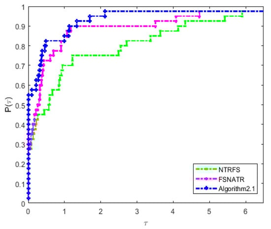
Figure 2. Performance profile for the number of gradient evaluations ($n_i$).

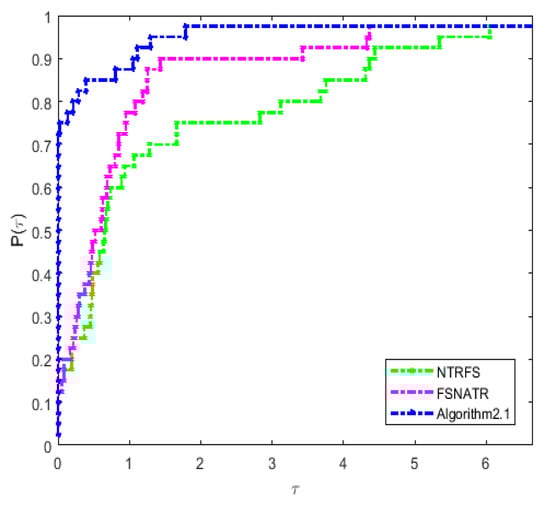
Figure 3. Performance profile for the number of function evaluations ($n_f$).

6. Conclusions

In this paper, the authors proposed a new nonmonotone trust region method and also put forward the following innovations:

(1) a new adaptive radius strategy to reduce the number of calculations;

(2) a modified trust region ratio to solve effectively unconstrained optimization problems. The filter technology is also important. Theorems 1 and 2 show that the proposed algorithm can preserve global convergence and superlinear convergence, respectively. According to preliminary numerical experiments, we can conclude that the new algorithm is very effective for unconstrained optimization, and the nonmonotone technology is very helpful for many optimization problems. In the future, we will have more ideas for solving many optimization problems, such as combining the modified conjugate gradient algorithm with a modified trust region method. We can also use the new algorithm for solving constrained optimization problems.

References

- Mo, J.T.; Zhang, K.C.; Wei, Z.X. A nonmonotone trust region method for unconstrained optimization. Appl. Math. Comput. 2005, 171, 371–384. [Google Scholar] [CrossRef]
- Ou, Y.G.; Zhou, Q.; Lin, H.C. An ODE-based trust region method for unconstrained optimization problems. J. Comput. Appl. Math. 2009, 232, 318–326. [Google Scholar] [CrossRef]
- Wang, X.Y.; Tong, J. A Nonmonotone Adaptive Trust Region Algorithm with Fixed Stepsize for Unconstrained Optimization Problems. Math. Appl. 2009, 3, 496–500. [Google Scholar]
- Hang, D.; Liu, M. On a Fixed Stepsize Nonmonotonic Self-Adaptive Trust Region Algorithm. J. Southwest China Norm. Univ. 2013, 38. [Google Scholar] [CrossRef]
- Sartenaer, A. Automatic determination of an initial trust region in nonlinear programming. SIAM J. Sci. Comput. 1997, 18, 1788–1803. [Google Scholar] [CrossRef]
- Zhang, X.S.; Zhang, J.L.; Liao, L.Z. An adaptive trust region method and its convergence. Sci. China 2002, 45, 620–631. [Google Scholar] [CrossRef]
- Shi, Z.J.; Guo, J.H. A new trust region methods for unconstrained optimization. Comput. Appl. Math. 2008, 213, 509–520. [Google Scholar] [CrossRef]
- Kimiaei, M. A new class of nonmonotone adaptive trust-region methods for nonlinear equations with box constraints. Calcolo 2017, 54, 769–812. [Google Scholar] [CrossRef]
- Amini, K.; Shiker Mushtak, A.K.; Kimiaei, M. A line search trust-region algorithm with nonmonotone adaptive radius for a system of nonlinear equations. Q. J. Oper. Res. 2016, 4, 132–152. [Google Scholar] [CrossRef]
- Peyghami, M.R.; Tarzanagh, D.A. A relaxed nonmonotone adaptive trust region method for solving unconstrained optimization problems. Comput. Optim. Appl. 2015, 61, 321–341. [Google Scholar] [CrossRef]
- Deng, N.Y.; Xiao, Y.; Zhou, F.J. Nonmonotone Trust Region Algorithm. J. Optim. Theory Appl. 1993, 76, 259–285. [Google Scholar] [CrossRef]
- Ahookhoosh, M.; Amini, K.; Peyghami, M. A nonmonotone trust region line search method for large scale unconstrained optimization. Appl. Math. Model. 2012, 36, 478–487. [Google Scholar] [CrossRef]
- Zhang, H.C.; Hager, W.W. A nonmonotone line search technique and its application to unconstrained optimization. SIAM J. Optim. 2004, 14, 1043–1056. [Google Scholar] [CrossRef]
- Gu, N.Z.; Mo, J.T. Incorporating nonmonotone strategies into the trust region for unconstrained optimization. Comput. Math. Appl. 2008, 55, 2158–2172. [Google Scholar] [CrossRef]
- Fletcher, R.; Leyffer, S. Nonlinear programming without a penalty function. Math. Program. 2002, 91, 239–269. [Google Scholar] [CrossRef]
- Gould, N.I.; Sainvitu, C.; Toint, P.L. A filter-trust-region method for unconstrained optimization. SIAM J. Optim. 2005, 16, 341–357. [Google Scholar] [CrossRef]
- Gould, N.I.; Leyffer, S.; Toint, P.L. A multidimensional filter algorithm for nonlinear equations and nonlinear least-squares. SIAM J. Optim. 2004, 15, 17–38. [Google Scholar] [CrossRef]
- Wächter, A.; Biegler, L.T. Line search filter methods for nonlinear programming and global convergence. SIAM J. Optim. 2005, 16, 1–31. [Google Scholar] [CrossRef]
- Miao, W.H.; Sun, W. A filter trust-region method for unconstrained optimization. Numer. Math. J. Chin. Univ. 2007, 19, 88–96. [Google Scholar]
- Zhang, Y.; Sun, W.; Qi, L. A nonmonotone filter Barzilai-Borwein method for optimization. Asia Pac. J. Oper. Res. 2010, 27, 55–69. [Google Scholar] [CrossRef]
- Fatemi, M.; Mahdavi-Amiri, N. A filter trust-region algorithm for unconstrained optimization with strong global convergence properties. Comput. Optim. Appl. 2012, 52, 239–266. [Google Scholar] [CrossRef]
- Nocedal, J.; Wright, S.J. Numerical Optimization; Springer: New York, NY, USA, 2006. [Google Scholar]
- Andrei, N. An unconstrained optimization test functions collection. Environ. Sci. Technol. 2008, 10, 6552–6558. [Google Scholar]
- Pang, S.; Chen, L. A new family of nonmonotone trust region algorithm. Math. Pract. Theory. 2011, 10, 211–218. [Google Scholar]
- Dolan, E.D.; Moŕe, J.J. Benchmarking optimization software with performance profiles. Math. Program. 2002, 91, 201–213. [Google Scholar] [CrossRef]
© 2020 by the authors. Licensee MDPI, Basel, Switzerland. This article is an open access article distributed under the terms and conditions of the Creative Commons Attribution (CC BY) license (http://creativecommons.org/licenses/by/4.0/).