Article

A New Bimodal Distribution for Modeling Asymmetric Bimodal Heavy-Tail Real Lifetime Data

by
Nadeem S. Butt
1 and
Mohamed G. Khalil
2,*
1
Department of Family and Community Medicine, Rabigh King Abdul Aziz University, 21589 Jeddah, Saudi Arabia
2
Department of Statistics, Mathematics and Insurance, Benha University, 13518 Benha, Egypt
*
Author to whom correspondence should be addressed.
Symmetry 2020, 12(12), 2058; https://doi.org/10.3390/sym12122058
Submission received: 14 November 2020 / Revised: 4 December 2020 / Accepted: 6 December 2020 / Published: 11 December 2020
(This article belongs to the Special Issue Symmetric and Asymmetric Bimodal Distributions with Applications)

Abstract

:
We introduced and studied a new generalization of the Burr type X distribution. Some of its properties were derived and numerically analyzed. The new density can be “right-skewed” and symmetric with “unimodal” and many “bimodal” shapes. The new failure rate can be “increasing,” “bathtub,” “J-shape,” “decreasing,” “increasing-constant-increasing,” “reversed J-shape,” and “upside-down (reversed U-shape).” The usefulness and flexibility of the new distribution were illustrated by means of four asymmetric bimodal right- and left-heavy tail real lifetime data.

1. Introduction

Burr [1] introduced twelve different forms of cumulative distribution functions (CDFs) for modeling real data sets. Among those twelve CDFs, Burr type X (BX) and Burr type XII (BXII) have received special attention. A random variable (RV) W is said to have the BX distribution if its probability density function (PDF), and hence the CDF, are given by:
π c 1 , c 2 ( w ) = 2 c 1 c 2 2 w e ( c 2 w ) 2 [ 1 e ( c 2 w ) 2 ] c 1 1 ,
and
Π c 1 , c 2 ( w ) = [ 1 e ( c 2 w ) 2 ] c 1 ,
Respectively, for W > 0 and c 1 , c 2 > 0 . For c 1 = 1 , we have the standard Rayleigh model. For c 2 = 1 , we have the one-parameter BX model (for more details see [2,3,4,5,6,7]). For c 1 = 1 , we have the Rayleigh (R) model. Recently, [8] observed that the BX model can be used in modeling strength and general lifetime data. Several aspects of the one-parameter ( c 2   = 1) BX distribution were studied by [9], who studied the Bayesian prediction bounds under the BX model, [10] presented the Bayesian approach for prediction with outliers from the BX model, and [11] and [7] investigated the inference for P(Y < X) in the BX model. Many authors have studied the BX distribution and applied it in different areas, e.g., [12] presented an overview about the BX model, [13] proposed a new version of the BX model called the beta Burr type X (BBX) distribution and discussed its relevant mathematical properties along with some real data applications, and [14] presented an estimation of reliability under the one-parameter BX model. [15] Proposed a new generator of distributions based on the BX model. [16] Compounded the Poisson model and the BX model and introduced a new compound generator called the Poisson BX family. Recently, [17] used the Weibull and the BX model to generate a new flexible model and presented a new modified Bagdonavičius–Nikulin goodness-of-fit test for censored validation; [18] presented the quasi Poisson BX-BX distribution along with copula, mathematical properties, and applications; [19] generalized the odd log-logistic BX distribution with an application to the times of failure and running times for a sample of devices from a field-tracking study of a larger system.
By examining the statistical literature, it is noted that all the proposed versions of the BX model have a unimodal density. In this work, we present a new bimodal version of the BX model called the odd Burr BX (OBBX) model based on the family from [20], who merged the generalized odd G (OG) family and the proportional reversed hazard rate family (PRHR) to propose a new wider family called the odd Burr G (OBG) family. The CDF of the OBG family is given by:
F ν , θ , ζ _ ( w ) = 1 Π ¯ ζ _ ( w ) ν θ [ Π ¯ ζ _ ( w ) ν + Π ζ _ ( w ) ν ] θ ,
where Π ¯ ζ _ ( w ) = 1 Π ζ _ ( w ) , ν and θ > 0 are two shape parameters, and ζ _ refers to the parameter vector of any baseline model and the reliability function (RF) of the baseline model. The PDF corresponding to (3) is given by:
f ν , θ , ζ _ ( w ) = ν θ π ζ _ ( w ) Π ζ _ ( w ) ν 1 Π ¯ ζ _ ( w ) ν θ 1 [ Π ¯ ζ _ ( w ) ν + Π ζ _ ( w ) ν ] 1 + θ .
For θ = 1 , the OBG family reduces to the OG family. For ν = 1 , the OBG family reduces to the PRHR. Using (3) and (4), the OBBX RF is given by:
S Θ _ ( w ) = [ 1 ( 1 O w , c 2 ) c 1 ] ν θ { ( 1 O w , c 2 ) c 1 ν + [ 1 ( 1 O w , c 2 ) c 1 ] ν } θ ,
where Θ _ = ν , θ , c 1 , c 2 ; O w , c 2 = e ( c 2 w ) 2 ; S Θ _ ( w ) = 1 F Θ _ ( w ) . For θ = 1 , the OBBX reduces to the O-BX. For ν = 1 , the OBBX reduces to the PRHR-BX. The PDF corresponding to (5) is given by:
f Θ _ ( w ) = 2 ν θ c 1 c 2 2 w   O w , c 2 ( 1 O w , c 2 ) c 1 ν 1 [ 1 ( 1 O w , c 2 ) c 1 ] ν θ 1 { ( 1 O w , c 2 ) c 1 ν + [ 1 ( 1 O w , c 2 ) c 1 ] ν } 1 + θ .
The hazard rate function (HRF) for the new model can be obtained from f Θ _ ( w ) / S Θ _ ( w ) . Many useful distributions are introduced based on the BX model, such as the BX Weibull (BXW) distribution [17], the Burr X Fréchet (BXFr) distribution [21], the Burr X exponentiated Weibull (BXEW) distribution [22], and the Burr X Nadarajah Haghighi (BXNH) distribution [23]. We were motivated to introduce and study the OBBX for the following reasons:
  • The new density in (6) can be “unimodal and right-skewed,” “symmetric and unimodal,” and “bimodal density” with many useful shapes (see Figure 1).
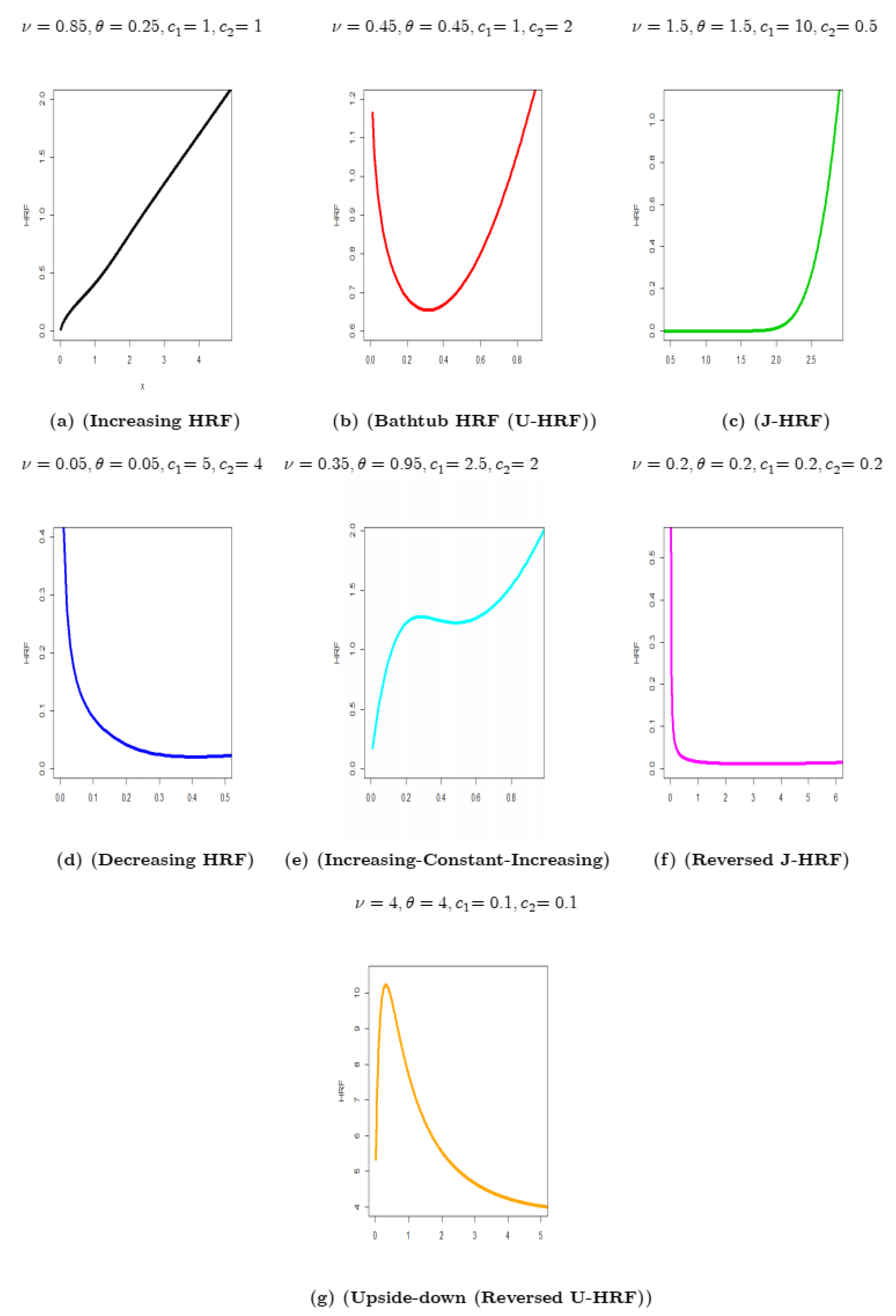
  • The HRF of the new model can be “monotonically increasing,” “bathtub (U-HRF),” “J-shaped (J-HRF),” “monotonically decreasing,” “increasing-constant-increasing,” “reversed J-HRF,” and “upside-down (reversed U-HRF)” (see Figure 2).
  • In reliability analysis, the OBBX model could be chosen as the best model, especially in modeling asymmetric bimodal failure times data and the asymmetric bimodal right-skewed and heavy-tail survival times data as illustrated in Section 5.1 and Section 5.3, respectively.
  • In medical fields, the OBBX model could be chosen as the best model, especially in modeling the bimodal right-skewed and heavy-tail cancer data, as illustrated in Section 5.2.
  • In engineering, the OBBX model could be chosen as the best model, especially in modeling the asymmetric bimodal left-skewed and heavy-tail glass fibers data, as shown in Section 5.4.
The asymptotic behavior of the CDF, PDF, and HRF as W 0 are respectively given by:
F Θ _ ( w ) | ( w 0 ) ~ θ ( 1 O w , c 2 ) c 1 ν ,
f Θ _ ( w ) | ( w 0 ) ~ 2 ν θ c 1 c 2 2 w   O w , c 2 ( 1 O w , c 2 ) c 1 ν 1 ,
and
h Θ _ ( w ) | ( w 0 ) ~ 2 ν θ c 1 c 2 2 w   O w , c 2 ( 1 O w , c 2 ) c 1 ν 1 .
The asymptotic behavior of the CDF, PDF, and HRF as W are respectively given by:
1 F Θ _ ( w ) | ( w ) ~ ν θ [ 1 ( 1 O w , c 2 ) c 1 ] θ ,
f Θ _ ( w ) | ( w ) ~ 2 ν θ θ c 1 c 2 2 w   O w , c 2 ( 1 O w , c 2 ) c 1 1 [ 1 ( 1 O w , c 2 ) c 1 ] 1 θ ,
and
h Θ _ ( w ) | ( w ) ~ 2 θ c 1 c 2 2 w   O w , c 2 ( 1 O w , c 2 ) c 1 1 1 ( 1 O w , c 2 ) c 1 .
Figure 1 gives some plots of the OBBX PDF for selected parameter values. Figure 2 gives some plots of the OBBX HRF for selected parameter values. Based on Figure 1, the new density can be “right-skewed” and symmetric with “unimodal” and many “bimodal” shapes. Based on Figure 2, the new HRF can take the following forms:
For the simulations of this new model, we obtained the quantile function (QF) of W (by inverting the CDF), say w u = F 1 ( u ) , as:
w u = 1 c 2 [ ln ( 1 { [ 1 ( 1 u ) 1 θ ] 1 ν ( 1 u ) 1 ν θ + [ 1 ( 1 u ) 1 θ ] 1 ν } 1 c 1 ) ] 1 2 ,
where (7) was used as the random number generator from the OBBX model.

2. Mathematical Properties

2.1. Useful Representations

Based on [20], the PDF in (6) can be expressed as:
f ( w ) = k 4 = 0 Υ k 4   π c 1 * , c 2 ( w ) | ( c 1 * = c 1 ( 1 + k 4 ) ) ,
where:
Υ k 4 = ν θ 1 + k 4 k 1 , k 2 = 0 k 3 = k 4 ( 1 ) k 2 + k + k 4 ( ( 1 + θ ) k 1 ) ( [ ν ( 1 + k 1 ) + 1 ] k 2 ) ( ν ( 1 + k 1 ) + k 2 + 1 k 3 ) , ( k 3 k 4 ) ,
and π c 1 * , c 2 ( w ) is the PDF of the BX model. By integrating (8), the CDF of W becomes:
F ( w ) = k 4 = 0 Υ k 4   Π c 1 * , c 2 ( w ) ,
where Π c 1 * , c 2 ( w ) refers to the CDF of the BX distribution.

2.2. Moments and Incomplete Moments

The r th ordinary moment of W is given by:
μ r = E ( W r ) =   w r   f ( w ) d w   .
Then, we obtain:
μ r | ( r > 2 ) = c 2 r Γ ( 1 + r 2 ) k 4 , h = 0 Υ k 4 , h ( r , c 1 * )   ,
where:
Υ k 4 , h ( r , c 1 * ) = Υ k 4   c 1 * ( 1 ) h ( h + 1 ) ( r + 2 ) / 2 ( c 1 * 1 h ) ,
and
Γ ( 1 + ϕ ) | ( ϕ + ) = ϕ ! = r = 0 ϕ 1 ( ϕ r ) ,
The variance (V ( W ) ), skewness (S ( W ) ), and kurtosis (K ( W ) ) can be derived easily using the well-known relationships. The r th incomplete moment, say I r ( τ ) , of W can be expressed, from (9), as:
I r ( τ ) = τ w r f ( w ) d w = k 4 = 0 Υ k 4 τ w r   π c 1 * , c 2 ( w ) d w .
Then:
I r ( τ ) | ( r > 2 ) = c 2 r γ ( 1 + r 2 , ( c 2 t ) 2 ) k 4 , h = 0 Υ k 4 , h ( r , c 1 * ) ,
where γ ( ϕ , ψ ) refers to the incomplete gamma function:
γ ( ϕ , ψ ) = 0 ψ w ϕ 1 e w d w = k = 0 ( 1 ) k 4 k 4 ! ( ϕ + k ) ψ ϕ + k .
The first incomplete moment is given by (11) with r = 1 as:
I 1 ( τ ) = c 2 γ ( 3 2 , ( c 2 t ) 2 ) k 4 , h = 0 Υ k 4 , h ( 1 , c 1 * )   .
The dispersion index (DisIx), also known as the variance-to-mean ratio, is a measure used to quantify whether a set of observed occurrences are clustered or dispersed compared to a standard statistical model. Therefore, it indicates whether a certain statistical model is suitable for over- (or under-) dispersed data sets and is used widely in ecology as a standard measure for measuring clustering (overdispersion) or repulsion (underdispersion). Thus, the measure can be used to assess whether observed data can be modeled using a Poisson process. For any real data set, when the DisIx is less than 1 , the data set is said to be “under-dispersed”; this important condition can relate to occurrence patterns that are more regular than the randomness associated with a Poisson process. Numerical analysis for the DisIx ( W ) of the new OBBX is presented in Table 1 with useful comments.

2.3. Moment Generating Function (MGF)

The MGF M W ( τ ) = E ( exp ( τ W ) ) of W can be derived from (8) as:
M W ( τ ) = k 4 = 0 v k 4   M c 1 * , c 2 ( τ ) ,
where M c 1 * ( τ ) is the MGF of the BX model. Then:
M W ( τ ) | ( r > 2 ) = r = 0 k 4 , h = 0 τ r r ! c 2 r Γ ( 1 + r 2 )   Υ k 4 , h ( r , c 1 * ) .

2.4. Residual Life and Reversed Residual Life Functions

The r th moment of the residual life A r ( τ ) = E [ ( W τ ) r | w > τ , r = 1 , 2 , ] . Then, the r th moment of the residual life of W is given by A r ( τ ) = 1 1 F ( τ )   τ ( W τ ) r d F ( w ) Therefore:
A r ( τ ) = 1 1 F ( τ ) k 4 , h = 0 a k 4 , h ( r , c 1 * ) c 2 r Γ ( 1 + r 2 , ( c 2 t ) 2 ) | ( r > 2 )   ,
where a k 4 , h ( r , c 1 * ) = Υ k 4 m = 0 r ( r m ) ( τ ) r m , Γ ( ϕ , r ) | r > 0 = r w ϕ 1 e w d w , and Γ ( ϕ , r ) = Γ ( ϕ ) γ ( ϕ , r ) .
The r th moment of the reversed residual life, say:
W r ( τ ) = E [ ( τ W ) r | w τ , τ > 0 and r = 1 , 2 , ] ,
uniquely determines F ( w ) . Then, we obtain:
W r ( τ ) = 1 F ( τ ) 0 τ ( τ W ) r d F ( w ) .
Then, the r th moment of the reversed residual life of W becomes:
W r ( τ ) = 1 F ( τ ) k 4 , h = 0 b k 4 , h ( r , c 1 * ) c 2 r γ ( 1 + r 2 , ( c 2 t ) 2 ) | ( r > 2 )   ,
where b k 4 , h ( r , c 1 * ) = Υ k 4 m = 0 r ( 1 ) m ( r m ) τ m r .

2.5. Numerical Analysis for the Mean, V ( W ) , S ( W ) , K ( W ) , and DisIx ( W ) .

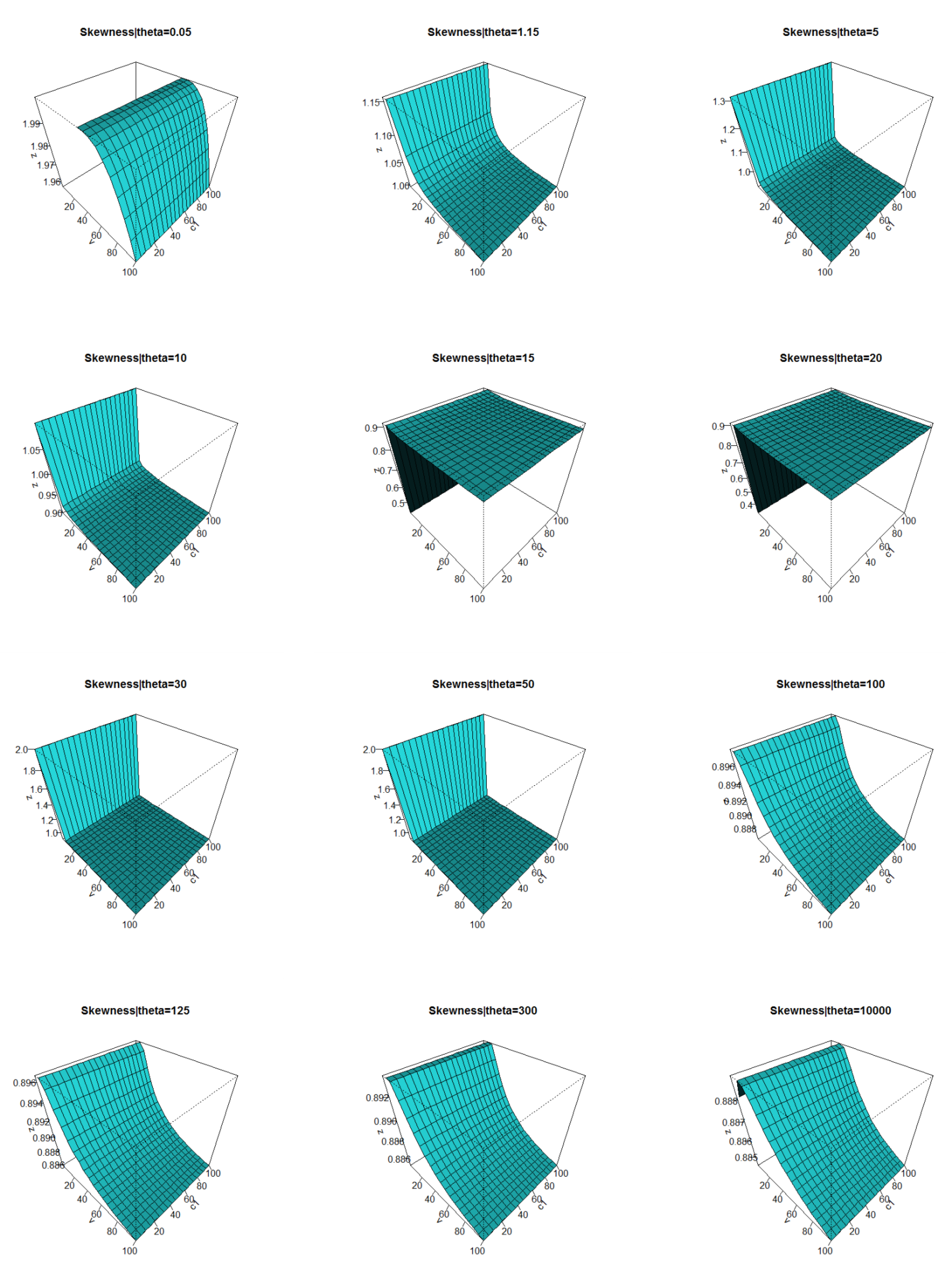
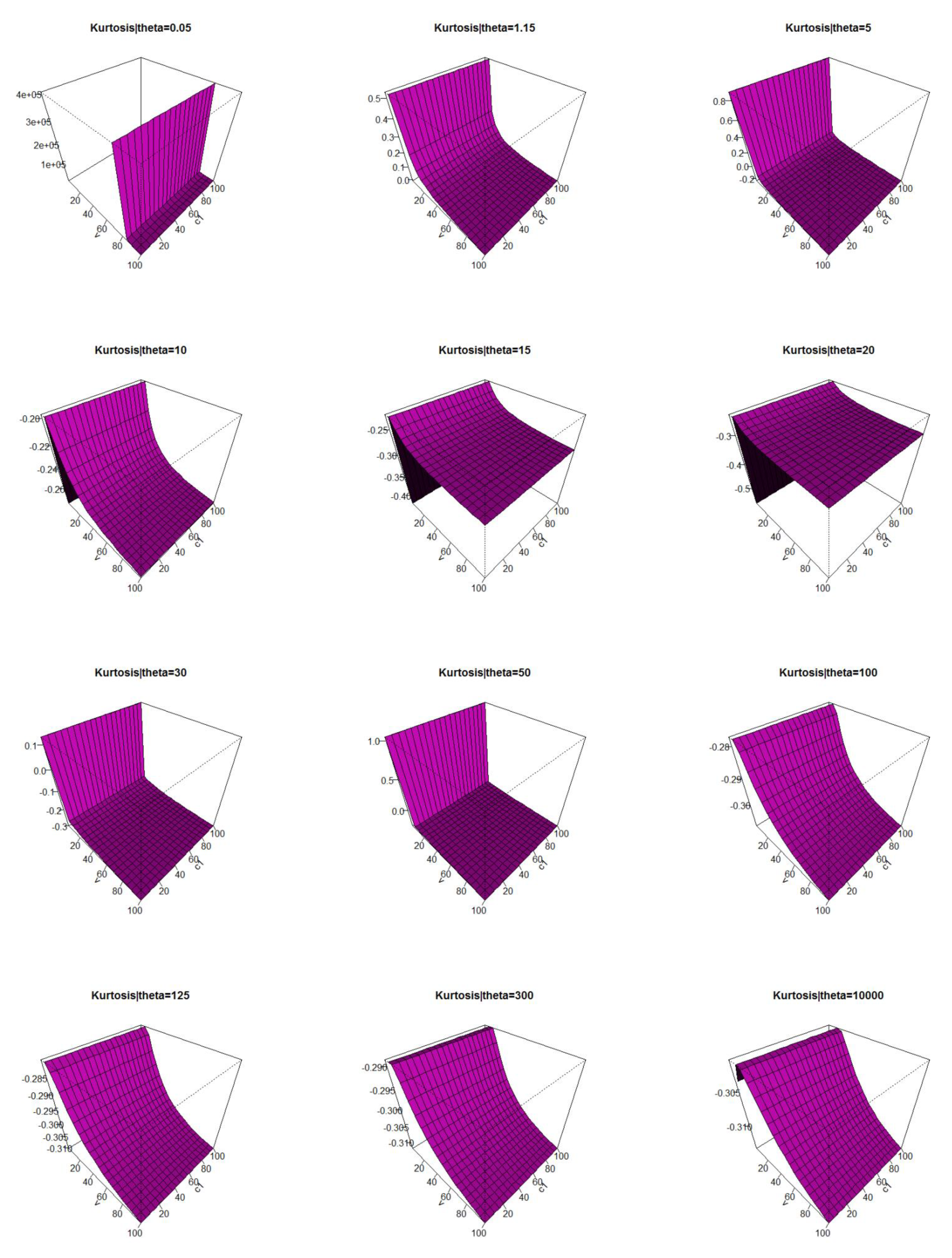
Table 1 gives numerical calculations for the mean, V ( W ) , S ( W ) , K ( W ) , and dispersion index (DisIx ( W ) ) for selected parameter values. Based on Table 1, we note that (1) the skewness of the OBBX model can be both positive and negative; (2) the spread for the OBBX kurtosis is much larger, ranging from 1.0005 to 172,196.5; (3) DisIx ( W ) can be “between 0 and 1 ” or “more than 1 .” For more visualization, Figure 3 gives some three-dimensional skewness plots and Figure 4 gives three-dimensional kurtosis plots.

3. Maximum Likelihood Estimation

The maximum likelihood estimations (MLEs) display desirable properties and can be used for establishing confidence intervals and test statistics. The normal approximation for MLEs in large sample theory is easily handled either numerically or analytically. In this section, we determine the MLEs of the parameters of the OBBX distribution from complete samples only. However, censored samples could be considered in separate works. Let w 1 ,   w 2 , …,   w n be an observed random sample from the OBBX model with parameters ν , θ , c 1 , and c 2 . Then, the log-likelihood function for Θ _ , say ( ν , θ , c 1 , c 2 ), is given by:
𝓛 ( Θ _ ) = n log 2 + n log ν + n log θ + n log c 1 + 2 n log c 2 + i = 0 n log w i + i = 0 n log ( O w i , c 2 ) + ( c 1 ν 1 ) i = 0 n log ( 1 O w i , c 2 ) ( 1 + θ ) i = 0 n log { 𝓺 i c 1 ν + [ 1 𝓺 i c 1 ] ν } + ( ν θ 1 ) i = 0 n log [ 1 𝓺 i c 1 ] ,
where 𝓺 i = 1 O w i , c 2 and O w i , c 2 = e ( c 2 w i ) 2 . The equation of 𝓛 ( Θ _ ) can be maximized either directly by using the R program via the optim function, the SAS program via PROC NLMIXED, or the Ox program using sub-routine MaxBFGS or by solving the nonlinear likelihood equations obtained by differentiating 𝓛 ( ν , θ , c 1 , c 2 ). The score vector components, say:
U ( Θ _ ) = ( Θ _ ) Θ _ = ( U ( ν ) , U ( θ ) , U ( c 1 ) , U ( c 2 ) ) T ,
are available from the corresponding author, where:
U ( ν ) = n ν + c 1 i = 0 n log 𝓺 i + θ i = 0 n log [ 1 𝓺 i c 1 ] ( 1 + θ ) i = 0 n c 1 𝓺 i c 1 ν log 𝓺 i + [ 1 𝓺 i c 1 ] ν log [ 1 𝓺 i c 1 ] 𝓺 i c 1 ν + [ 1 𝓺 i c 1 ] ν , U ( θ ) = n θ i = 0 n log { 𝓆 i c 1 ν + [ 1 𝓆 i c 1 ] ν } + ν i = 0 n log [ 1 𝓆 i c 1 ] ,
U ( c 1 ) = n c 1 + ν i = 0 n log 𝓺 i + ( ν θ 1 ) i = 0 n 𝓺 i c 1 log 𝓺 i 1 𝓺 i c 1 ( 1 + θ ) i = 0 n ν 𝓆 i c 1 ν log 𝓆 i + [ 1 𝓆 i c 1 ] ν log [ 1 𝓆 i c 1 ] 𝓆 i c 1 ν + [ 1 𝓆 i c 1 ] ν ,
U ( c 2 ) = 2 n c 2 + i = 0 n 2 c 2   w i 2 O w i , c 2 O w i , c 2 + 2 c 2 ( c 1 ν 1 ) i = 0 n   w i 2 O w i , c 2 1 O w i , c 2 2 c 2 ( ν θ 1 ) i = 0 n   w i 2 O w i , c 2 𝓺 i c 1 1 1 𝓺 i c 1 ( 1 + θ ) i = 0 n 2 c 1 c 2 ν O w i , c 2 w i 2 𝓆 i c 1 ν 1 2 c 2 ν w i 2 O w i , c 2 𝓆 i c 1 1 [ 1 𝓆 i c 1 ] ν 1 𝓆 i c 1 ν + [ 1 𝓆 i c 1 ] ν .
Setting the nonlinear system of equations to U ( ν ) = U ( θ ) = U ( c 1 ) = U ( c 2 ) = 0 and solving them simultaneously yields the MLEs. These equations cannot be solved analytically, but Newton–Raphson-type algorithms can be used to solve them numerically (see the Appendix A). For the interval estimation of the OBBX model parameters, we require the observed information matrix J( Θ _ ), which comes as the output using the above maximization procedures. Likelihood ratio tests can be performed for the proposed model in the usual way. Further works could be addressed using different estimation methods to estimate the parameters of the OBBX model, such as bootstrap, least squares, Cramér–von Mises, weighted least squares, Jackknife, Anderson–Darling, Bayesian analysis, and compare the estimators based on these methods.

4. Graphical Assessment

Graphically and using the biases and mean squared errors (MSEs), we can perform the simulation experiments to assess the finite sample behavior of the MLEs given in Section 4. The assessment was based on the following algorithm (see the Appendix A):
  • N = 1000 samples of size n | ( n   =   50 ,   100 ,   ,   2000 ) were generated from the OBBX distribution using (7);
  • The MLEs for N = 2000 samples, say [ ν ^ , θ ^ , ( c 1 ) ^ , ( c 2 ) ^ ] | ( = 1 , 2 , , 2000 ) were computed.
  • The SEs of the MLEs for the 2000 samples, say [ S ν ^ , S θ ^ , S ( c 1 ) ^ , S ( c 2 ) ^ ] | ( = 1 , 2 , , 2000 ) were computed by inverting the observed information matrix.
  • The biases and mean squared errors given for Θ _ = ν , θ , c 1 , c 2 . We repeated these steps for n | ( n = 50 , 100 , , 2000 ) with ν = 1 ,   2 , ,   100 ;   θ = 1 ,   2 , ,   100 ;   c 1 = 1 ,   2 , ,   100 ;   c 2 = 1 , 2,…, 100 to compute the biases ( Bias Θ _ ( n ) ) and mean squared errors ( MSEs ) ( MSE h ( n ) ) for Θ _ = ν , θ , c 1 , c 2 and n | ( n = 50 , 100 , , 2000 ) where Bias Θ _ ( n ) | ( Θ _ = ν , θ , c 1 , c 2 ) = 1 1000 = 1 1000 ( Θ _ ^ Θ _ ) and MSE Θ _ ( n ) | ( Θ _ = ν , θ , c 1 , c 2 ) = 1 1000 = 1 1000 ( Θ _ ^ Θ _ ) 2 .
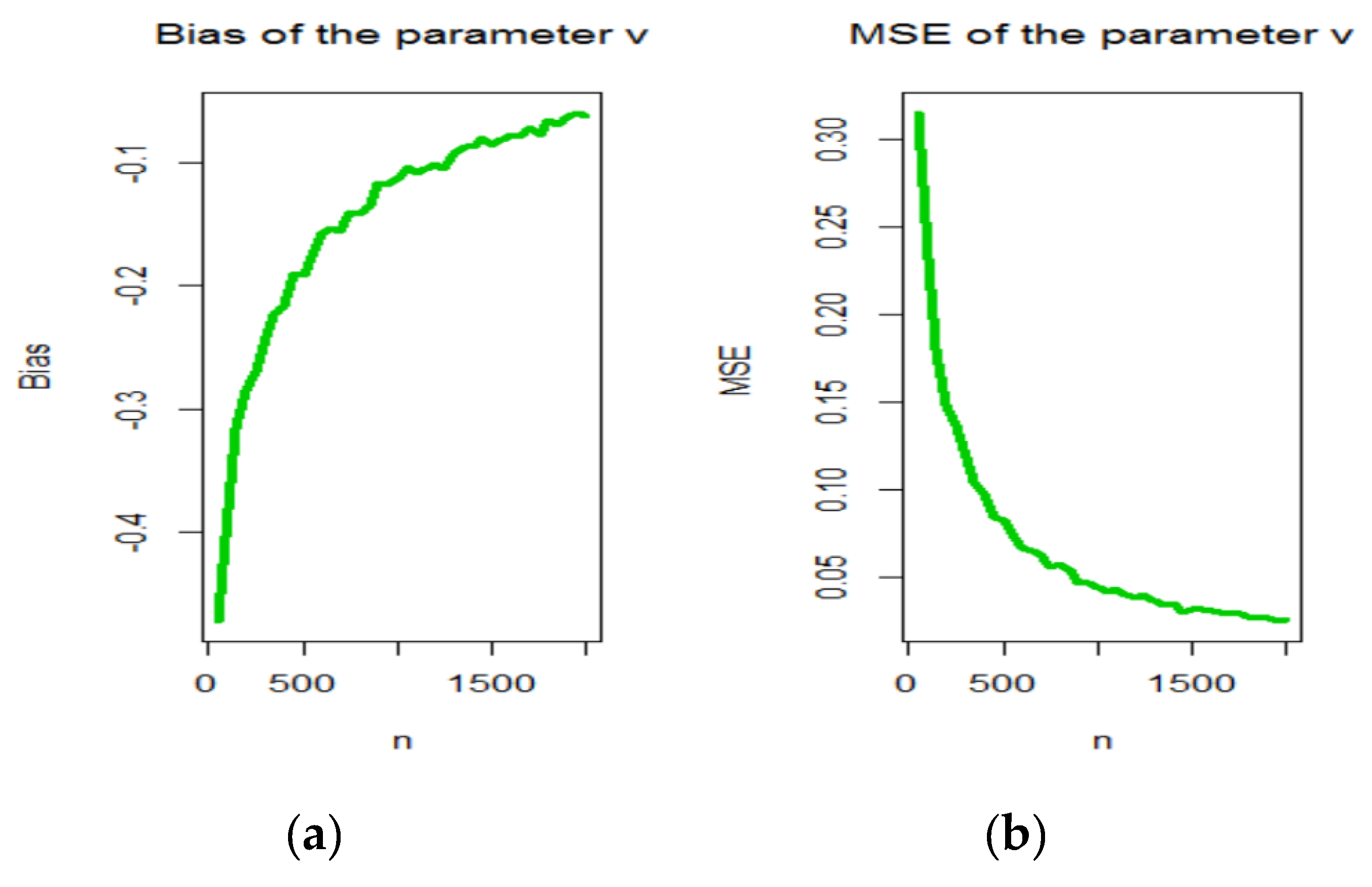
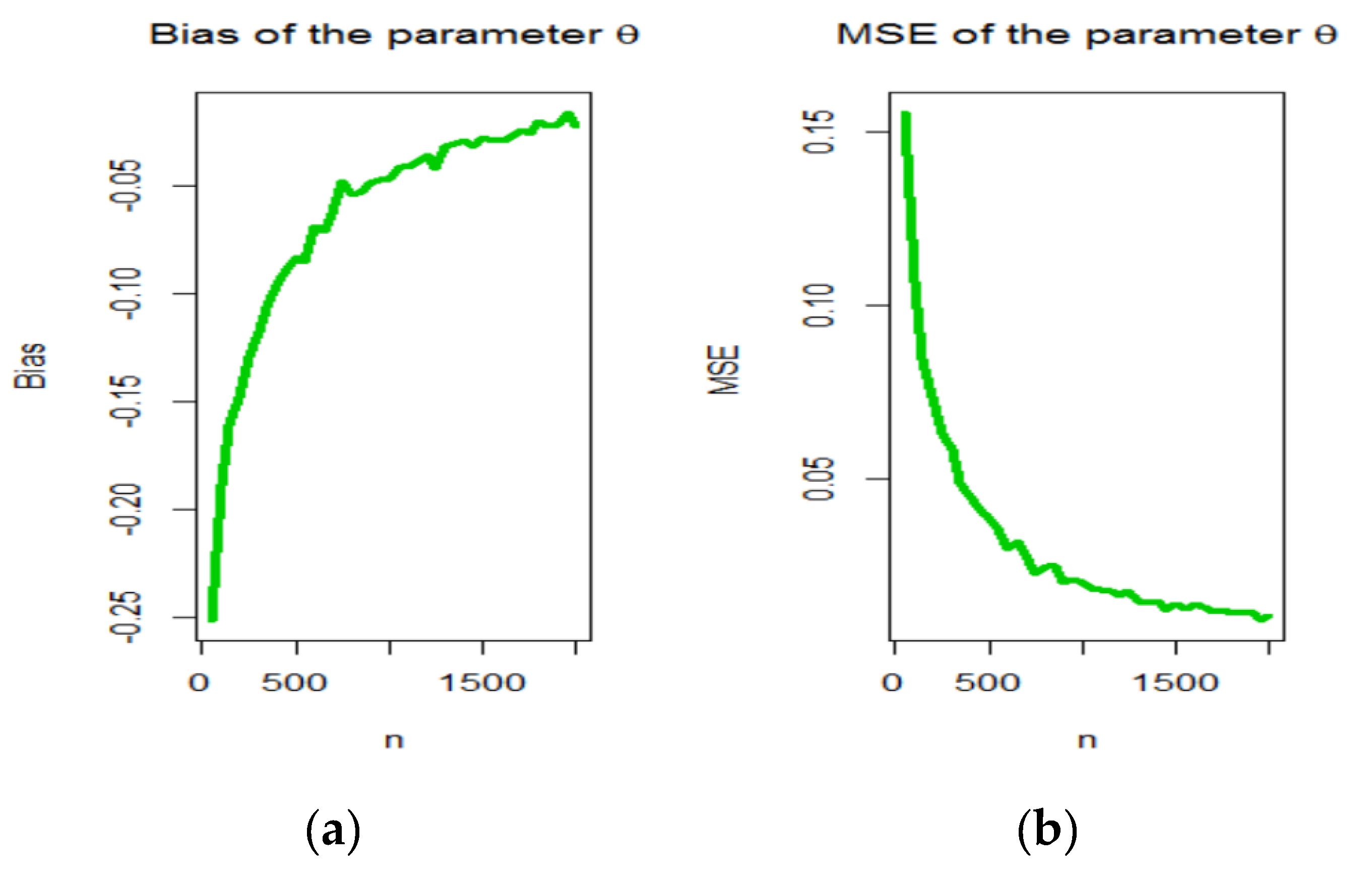
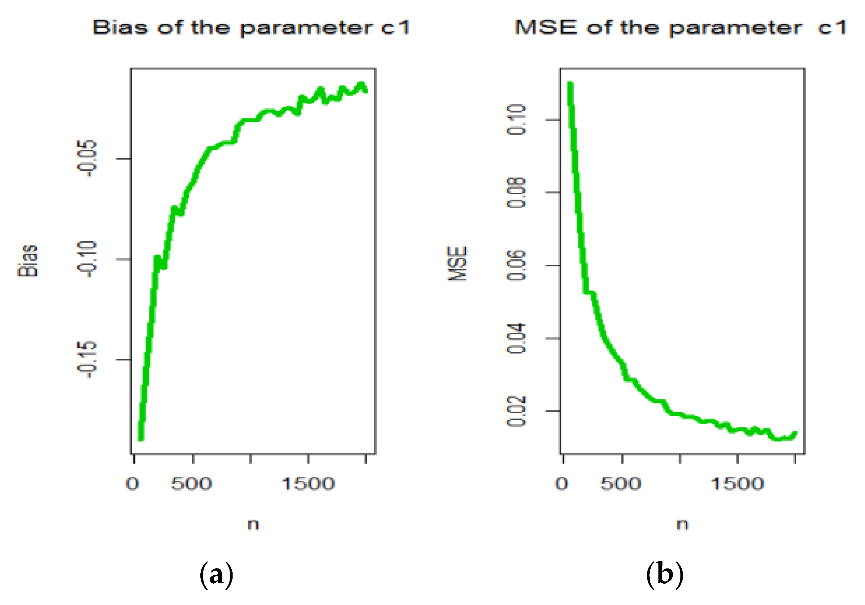
Figure 5, Figure 6, Figure 7 and Figure 8a give the biases for the four parameters, where they illustrate how the biases vary with respect to n . Figure 5, Figure 6, Figure 7 and Figure 8b give the MSEs for the four parameters, where they illustrate how the four MSEs vary with respect to n . The broken red line in Figure 8 corresponds to the biases being 0 . From Figure 5, Figure 6, Figure 7 and Figure 8, the biases for each parameter were generally “negative” and decrease to 0 as m , while the MSEs for each parameter decrease to zero as n .

5. Applications

In this section, we provide four applications of the OBBX distribution to empirically show its potentiality. In order to compare the fits of the OBBX distribution with other competing distributions, we consider the Cramér–von Mises (CVM), the Anderson–Darling (AD), and the Kolmogorov–Smirnov (KS) (and its corresponding p-value) estimation methods. These four methods are widely used to determine how closely a specific CDF fits the empirical distribution of a given data set. The smaller the resulting statistics are, the better the fit. The required computations were carried out using the R software. For data set I: the MLEs and the corresponding standard errors ((SEs) in parentheses) for all the competitive parameters are given in Table 2, the numerical values of the statistics from CVM, AD, and KS (corresponding p-value) are listed in Table 3. For data set II: the MLEs and SEs in for all the competitive parameters are given in Table 4, the numerical values of the statistics from CVM, AD, and KS (corresponding p-value) are listed in Table 5. For data set III: the MLEs and SEs in for all the competitive parameters are given in Table 6, the numerical values of the statistics from CVM, AD, and KS (corresponding p-value) are listed in Table 7. For data set IV: the MLEs and SEs in for all the competitive parameters are given in Table 8, the numerical values of the statistics from CVM, AD, and KS (corresponding p-value) are listed in Table 9.
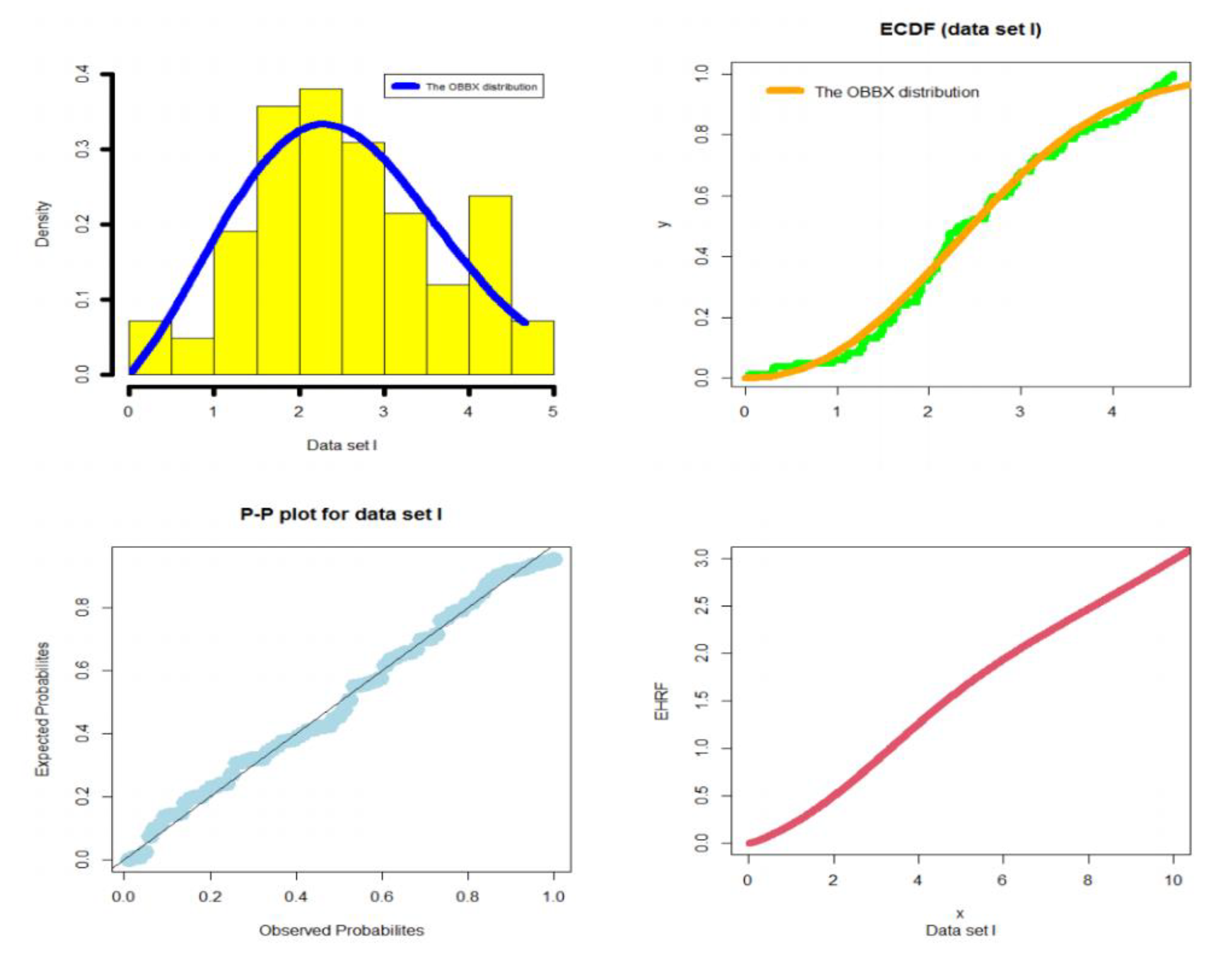
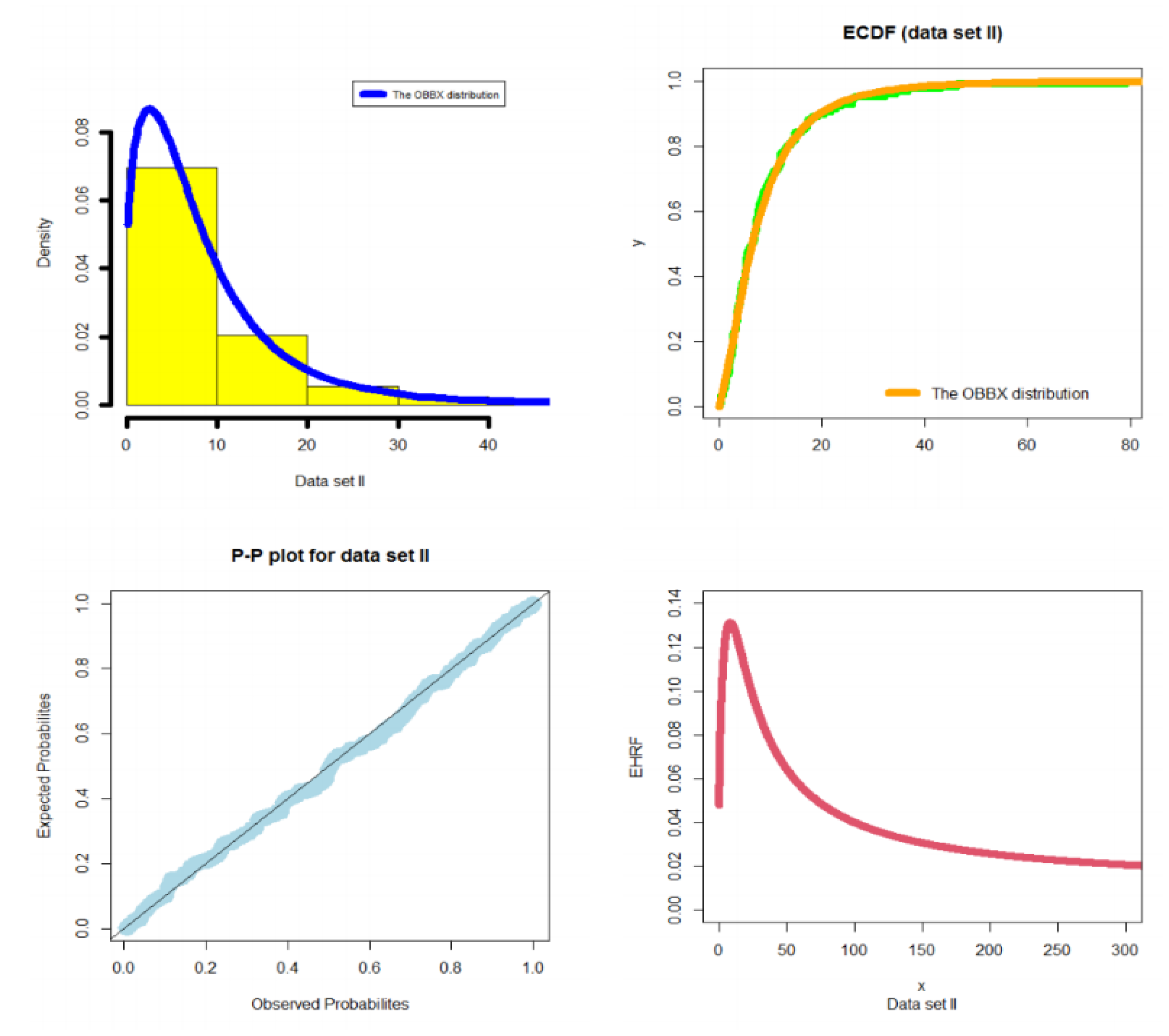
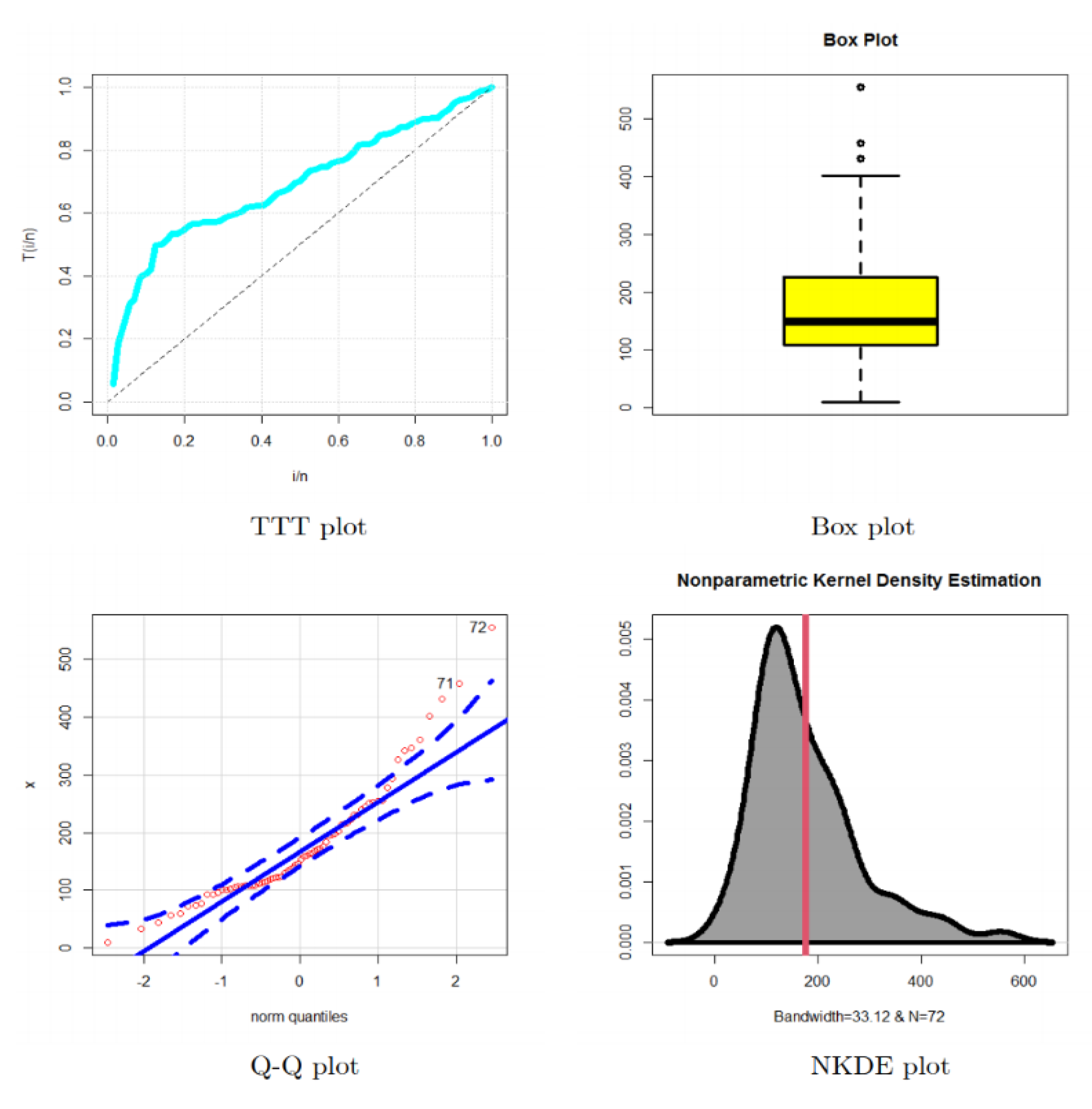
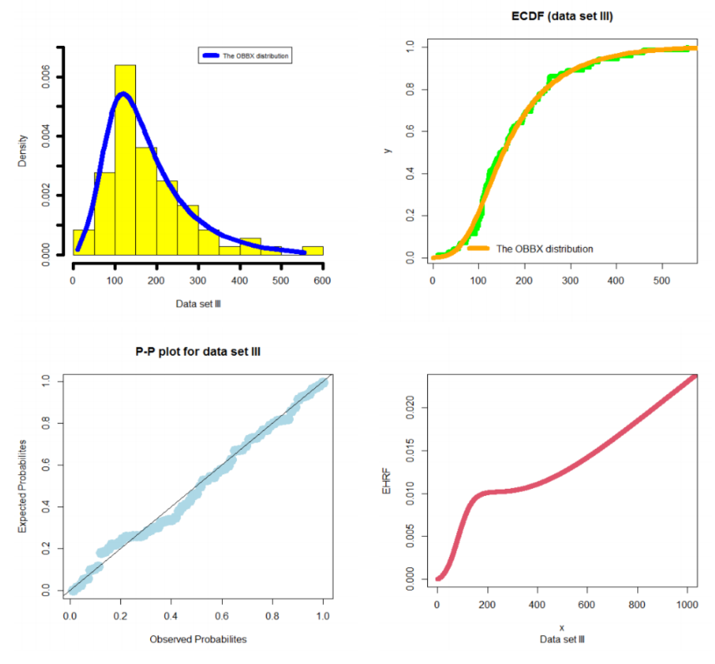
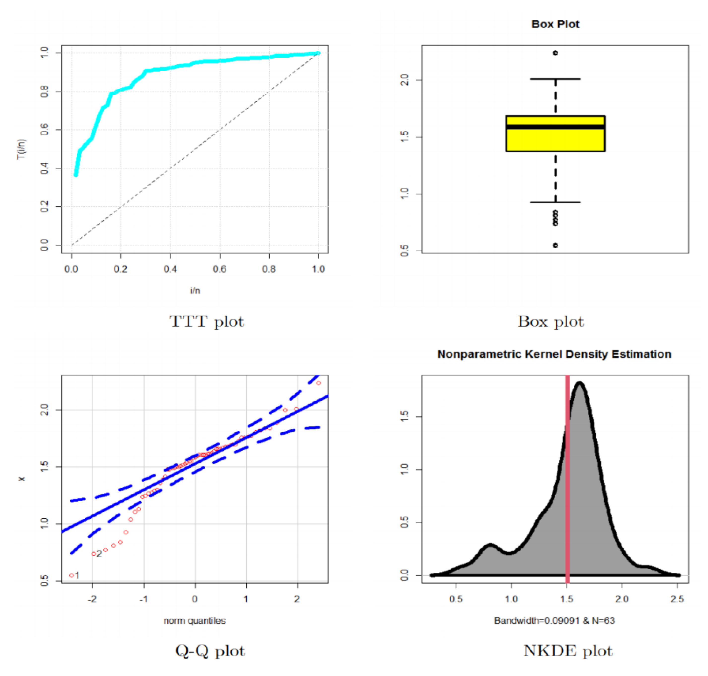
The total time in test (TTT) plot, box plot, quantile–quantile (Q-Q) plot, and the nonparametric Kernel density estimation (NKDE) plot for data set I are displayed in Figure 9. The estimated PDF (EPDF), estimated CDF (ECDF), probability–probability (P-P), and estimated HRF (EHRF) plots for data set I are displayed in Figure 10. The TTT, box plot, Q-Q and the NKDE plots for data set II are displayed in Figure 11. The EPDF, ECDF, P-P and EHRF plots for data set II are displayed in Figure 12. The TTT, box plot, Q-Q and the NKDE plots for data set II are displayed in Figure 13. The EPDF, ECDF, P-P and EHRF plots for data set III are displayed in Figure 14. The TTT, box plot, Q-Q and the NKDE plots for data set II are displayed in Figure 15. The EPDF, ECDF, P-P and EHRF plots for data set IV are displayed in Figure 16. The dashed line in all the Q-Q plots refers to the safe boundaries for the standard errors. The TTT plots show that the HRFs were “increasing” (data set I), “upside-down” (data set II), “increasing” (data set III), and “increasing” (data set IV). The box plots show that data sets II, III, and IV had some extreme values. The Q-Q plots ensure the results of the box plots. The NKDE plots show that the kernel density estimation was “asymmetric bimodal” (data set I), “asymmetric bimodal with a right-heavy tail” (data sets II and III), and “asymmetric bimodal with a left-heavy tail” (data sets IV). The R codes are given in see Appendix A.

5.1. Modeling Failure Times

The data consisted of 84 observations. Here, we shall compare the fits of the OBBX distribution with those of other competitive models, namely, the BX [1], odd Lindley exponentiated W (OLEW) [24], Burr X EW (BXEW) [22], Poisson Topp Leone W (PTLW) [25], Marshall Olkin extended-W (MOEW) [26], gamma-W (GamW) [27], Kumaraswamy-W (KumW) [28], beta-W [29], transmuted modified-W (TrMW) [30], modified beta-W (MBW) [31], Mcdonald-W (MacW) [32], and transmuted exponentiated generalized W (TrEGW) [33] distributions. Some other extensions of the W distribution can also be used in this comparison, but are not limited to [34,35,36,37,38,39,40,41,42,43]. Figure 9 presents the TTT, box, Q-Q, and NKDE plots for data set I. Figure 10 shows the EPDF, ECDF, P-P, and EHRF plots for data set I. Table 2 provides the MLEs (SEs) for data set I. Table 3 gives the CVM, AD, and KS (p-value) for data set I. Based on the values in Table 3 and Figure 10, we concluded that the new lifetime model provided adequate fits compared to other W models with small values for CVM and AD. The proposed OBBX lifetime model was much better than the BXEW, PTLW, MOEW, GamW, KumW, Beta-W, TrMW, KumTrW, MBW, MacW, and TrEGW models, and is a good alternative to these models.

5.2. Modeling Cancer Data

This data set represents the remission times (in months) of a random sample of 128 bladder cancer patients as reported in [44]. We compared the fits of the OBBX distribution with other competitive models, namely, the BX, Weibull (W) [45], TrMW, MBW, and transmuted additive W distribution (TrAW) ([34]) distributions with corresponding densities (for W > 0 ). Figure 11 presents the TTT, box, Q-Q, and NKDE plots for data set II. Figure 12 shows the EPDF, ECDF, P-P, and EHRF plots for data set II. Table 4 provides the MLEs (SEs) for data set II. Table 5 gives the CVM, AD, and KS (p-value) for data set II. Based on Table 5 and Figure 12, we concluded that the proposed OBBX lifetime model was much better than the W, TrMW, MBW, TrAW, and ETrGR models with small values for Cr [ 1 ] and Cr [ 2 ] in modeling cancer patient data.

5.3. Modeling Survival Times

The second real data set corresponds to the survival times (in days) of 72 guinea pigs infected with virulent tubercle bacilli reported by [46]. We compared the fits of the OBBX distribution with those of other competitive models, namely, the BX, transmuted (TrBX), OLEW, Odd W–W (OWW) [47], gamma exponentiated-exponential (GaEE) [48] distributions with PDFs (for W > 0 ). Figure 13 presents the TTT, box, Q-Q, and NKDE plots for data set III. Figure 15 shows the EPDF, ECDF, P-P, and EHRF plots for data set III. Table 6 provides the MLEs (SEs) for data set III. Table 7 gives the CVM, AD, and KS (p-value) for data set III. Based on Table 7 and Figure 15, we concluded that the proposed OBBX model was much better than all these models and was a good alternative to these models for modeling the survival times of guinea pigs.

5.4. Glass Fibers Data

This data consists of 63 observations of the strengths of 1.5 cm glass fibers, originally obtained by workers at the U.K. National Physical Laboratory. These data are given in [49]. For this data set, we compared the fits of the new distribution with some competitive models, such as the BX, TrBX, OLBX, OLEW, EW, TrW, and the odd log–logistic Weibull (OLLW) models. Figure 15 presents the TTT, box, Q-Q, and NKDE plots for data set IV. Figure 16 shows the EPDF, ECDF, P-P, and EHRF plots for data set IV. Table 8 provides the MLEs (SEs) for data set IV. Table 9 gives the CVM, AD, and KS (p-value) for data set IV. Based on Table 9 and Figure 16, we concluded that the proposed OBBX model was much better than all the competitor models and was a good alternative to these models in modeling glass fibers data.

6. Concluding Remarks

We introduced and studied a new generalization of the Burr type X distribution called the odd Burr–Burr type X (OBBX) distribution. Some of its properties were derived and numerically analyzed. The new PDF of the OBBX model was re-expressed in terms of the standard BX model. Graphically, we assessed the performance of the estimation method by means of biases and mean squared errors. The usefulness and flexibility of the new distribution was illustrated by means of four real data sets. The superiority of the new model against many other competitor models was proved using the Cramér–von Mises, the Anderson–Darling, and the Kolmogorov–Smirnov (and its corresponding p-value) statistics. The following concluding remarks can be made:
  • The new density can be “unimodal and right-skewed,” “symmetric and unimodal,” and “bimodal density” with many useful shapes.
  • The HRF of the new model can be “monotonically increasing,” “bathtub (U-HRF),” “J-HRF,” “monotonically decreasing,” “increasing-constant-increasing,” “reversed J-HRF,” and “upside-down (reversed U-HRF).”
  • In the reliability analysis, the OBBX model could be chosen as the best model, especially for modeling the asymmetric bimodal failure times data and the asymmetric bimodal right-skewed and heavy-tail survival times data.
  • In medical fields, the OBBX model could be chosen as the best model, especially for modeling the bimodal right-skewed and heavy-tail cancer data.
  • In engineering, the OBBX model could be chosen as the best model, especially for modeling the asymmetric bimodal left-skewed and heavy-tail glass fibers data.
  • In modeling the failure times data, the OBBX model showed its superiority against the Burr type X, odd Lindley exponentiated Weibull, Burr X exponentiated Weibull, Poisson Topp Leone Weibull, Marshall Olkin extended Weibull, Gamma Weibull Kumaraswamy Weibull, beta Weibull, transmuted modified Weibull, modified beta Weibull, Mcdonald Weibull, and the transmuted exponentiated generalized Weibull distributions.
  • In modeling the cancer data, the OBBX model showed its superiority against the Burr type X, Weibull, transmuted modified Weibull, modified beta Weibull, and transmuted additive Weibull distributions.
  • In modeling the survival data, the OBBX model showed its superiority against the Burr type X, transmuted Burr type X, odd Lindley exponentiated Weibull, odd Weibull–Weibull, and gamma-exponentiated exponential distributions.
  • In modeling the glass fibers data, the OBBX model showed its superiority against the Burr type X, transmuted Burr type X, odd Lindley Burr type X, odd Lindley exponentiated Weibull, exponentiated Weibull, transmuted Weibull, and odd log–logistic Weibull distributions.
Future works could be allocated for defining and studying many other Burr type X model versions using some well-known G families, such as the type I general exponential class of distributions [50], new extended G family of continuous distributions [51], and the type II general exponential class of distributions [52]. Based on [53], useful details about the computation of the probability associated with the Anderson–Darling statistic are given. Future works could use the approach of [53] as an alternative GOF statistics test.

Author Contributions

N.S.B.: software, validation, conceptualization, methodology, and writing—review and editing. M.G.K.: software, validation, conceptualization, methodology, writing—review and editing, and writing the original draft. All authors have read and agreed to the published version of the manuscript.

Funding

This research was funded by the Deanship of Scientific Research (DSR), at King Abdulaziz University, Jeddah, Kingdom of Saudi Arabia.

Acknowledgments

This Project was funded by the Deanship of Scientific Research (DSR), at King Abdulaziz University, Jeddah, Kingdom of Saudi Arabia. The authors, therefore, acknowledge with thanks DSR for technical and financial support.

Conflicts of Interest

The authors declare no conflict of interest.

Abbreviations

The following abbreviations are used in this manuscript:
PDFProbability density function
CDFCumulative distribution function
RFReliability function
MGFMoment generating function
HRFHazard rate function
MLEMaximum likelihood estimation
MSEMean square error
P-PProbability–probability
TTTTotal time in test
RVRandom variable
BXBurr type X
BXIIBurr type XII
O-GOdd G family
OBGOdd Burr-G family
OBBXOdd Burr–Burr type X model
PRHRProportional reversed hazard rate family
O-BXOdd Burr type X
PRHR-BXProportional reversed hazard rate Burr type X model
QFQuantile function
DisIxDispersion index
V(W)Variance
S(W)Skewness
K(W)Kurtosis
EPDFEstimated probability density function
ECDFEstimated cumulative distribution function
EHRFEstimated hazard rate function
Q-QQuantile–quantile plot
NKDENonparametric kernel density estimation plot

Appendix A

R Codes for Applications:
x = c(0.040, 1.866, 2.385, 3.443, 0.301, 1.876, 2.481, 3.467, 0.309, 1.899, 2.610, 3.478, 0.557, 1.911, 2.625, 4.570, 1.652, 2.300, 3.344, 4.602, 1.757, 3.578, 0.943, 1.912, 2.632, 3.595, 1.070, 1.914, 2.646, 3.699, 1.124, 1.981, 2.661, 3.779, 1.248, 2.010, 2.224, 3.117, 4.485, 1.652, 2.229, 3.166, 2.688, 3.924, 1.281, 2.038, 2.823, 4.035, 1.281, 2.085, 2.890, 4.121, 1.303, 2.089, 2.902, 4.167, 1.432, 4.376, 1.615, 2.223, 3.114, 4.449, 1.619, 2.097, 2.934, 4.240, 1.480, 2.135, 2.962, 4.255, 1.505, 2.154, 2.964, 4.278, 1.506, 2.190, 3.000, 4.305, 1.568, 2.194, 3.103, 2.324, 3.376, 4.663)
x = c(0.08, 2.09, 3.48, 4.87, 6.94,8.66, 13.11, 23.63, 0.20, 2.23, 3.52, 4.98, 6.97, 9.02, 13.29, 0.40, 2.26, 3.57, 5.06, 7.09, 9.22, 13.80,25.74, 0.50, 2.46, 3.64, 5.09, 7.26, 9.47, 14.24, 25.82, 0.51, 2.54, 3.70, 5.17, 7.28, 9.74, 14.76, 26.31,0.81, 2.62, 3.82, 5.32, 7.32, 10.06, 14.77, 32.15, 2.64, 3.88, 5.32, 7.39,10.34, 14.83, 34.26, 0.90, 2.69, 4.18, 5.34, 7.59, 10.66, 15.96, 36.66, 1.05, 2.69, 4.23, 5.41, 7.62, 10.75, 16.62, 43.01, 1.19, 2.75, 4.26, 5.41, 7.63, 17.12, 46.12, 1.26, 2.83, 4.33, 5.49, 7.66, 11.25, 17.14, 79.05, 1.35, 2.87, 5.62, 7.87, 11.64, 17.36, 1.40, 3.02, 4.34, 5.71, 7.93, 11.79, 18.10, 1.46, 4.40, 5.85, 8.26, 11.98, 19.13, 1.76, 3.25, 4.50, 6.25, 8.37, 12.02, 2.02, 3.31, 4.51, 6.54, 8.53, 12.03, 20.28, 2.02, 3.36, 6.76, 12.07, 21.73, 2.07, 3.36, 6.93, 8.65, 12.63, 22.69)
x = c(10, 33, 44, 56, 59, 72,74, 77, 92, 93, 96, 100, 100, 102, 105, 107, 107,108, 108, 108, 109, 112, 113, 115, 116, 120, 121, 122, 122, 124, 130, 134, 136,139, 144, 146, 153, 159, 160, 163, 163, 168, 171, 172, 176, 183, 195, 196, 197,202, 213, 215, 216, 222, 230,231, 240, 245, 251, 253, 254, 255, 278, 293, 327, 342, 347, 361, 402, 432, 458, 555)
x = c(0.55, 0.74, 0.77, 0.81, 0.84, 0.93, 1.04, 1.11, 1.13, 1.24, 1.25, 1.27, 1.28, 1.29, 1.30, 1.36, 1.39, 1.42, 1.48, 1.48, 1.49, 1.49, 1.50, 1.50, 1.51, 1.52, 1.53, 1.54, 1.55, 1.55, 1.58, 1.59, 1.60, 1.61, 1.61, 1.61, 1.61, 1.62, 1.62, 1.63, 1.64, 1.66, 1.66, 1.66, 1.67, 1.68, 1.68, 1.69, 1.70, 1.70, 1.73, 1.76, 1.76, 1.77, 1.78, 1.81, 1.82, 1.84, 1.84, 1.89, 2.00, 2.01, 2.24)
hist(x)
#=======================================
cdf_OBBX<- function(par,x){
v = par[1]
theta = par[2]
c1 = par[3]
c2 = par[4]
g.BX=(v*theta*((c2^2)*c1*2*x*exp(−(x*c2)^2)*((1 − exp(−(x*c2)^2))^(c1−1)))*(((1 − exp((x*c2)^2))^(c1))^(v−1))*((1 − ((1 − exp(−(x*c2)^2))^(c1)))^((v*theta)−1)))/(((((1 − exp((x*c2)^2))^(c1))^v)+((1 − ((1 − exp(−(x*c2)^2))^(c1)))^v))^(theta+1))
G.BX=1 − (((1 − ((1 − exp(−(x*c2)^2))^(c1)))^(v*theta))/(((((1 − exp(−(x*c2)^2))^(c1))^v)+((1 − ((1 − exp((x*c2)^2))^
  • (c1)))^v))^theta))
return(cdf)
}
pdf_OBBX <- function(par,x){
v = par[1]
theta = par[2]
c1 = par[3]
c2 = par[4]
g.BX=(v*theta*((c2^2)*c1*2*x^(2−1)*exp(−(x*c2)^2)*((1 − exp(−(x*c2)^2))^(c1−1)))*(((1 − exp((x*c2)^2))^(c1))^(v−1))*((1 − ((1-
exp(−(x*c2)^2))^(c1)))^((v*theta)−1)))/(((((1 − exp(−(x*c2)^2))^(c1))^v)+((1 − ((1 − exp(−(x*c2)^2))^(c1)))^v))^(theta+1))
G.BX=1 − (((1 − ((1 − exp(−(x*c2)^2))^(c1)))^(v*theta))/(((((1 − exp(−(x*c2)^2))^(c1))^v)+((1 − ((1 − exp(−(x*c2)^2))^(c1)))^v))^theta))
return(pdf)
}
Goodness-fit(pdf = pdf_OBBX, cdf = cdf_OBBX, starts = c(),,method = “select a numerical method”, domain = c(0,Inf), MLE = NULL)
2.
#=======================================
R Codes for Simulations:
cdf_OBBX<- function(par,x){
v = par[1]
theta = par[2]
c1 = par[3]
c2 = par[4]
g.BX=(v*theta*((c2^2)*c1*2*x^(2−1)*exp(−(x*c2)^2)*((1 − exp(−(x*c2)^2))^(c1−1)))*(((1 − exp((x*c2)^2))^(c1))^(v−1))*((1 − ((1 − exp(−(x*c2)^2))^(c1)))^((v*theta)−1)))/(((((1 − exp((x*c2)^2))^(c1))^v)+((1 − ((1 − exp(−(x*c2)^2))^(c1)))^v))^(theta+1))
G.BX=1 − (((1 − ((1 − exp(−(x*c2)^2))^(c1)))^(v*theta))/(((((1 − exp(−(x*c2)^2))^(c1))^v)+((1 − ((1 − exp((x*c2)^2))^
3.
(c1)))^v))^theta))
return(cdf)
}
pdf_OBBX <- function(par,x){
v = par[1]
theta = par[2]
c1 = par[3]
c2 = par[4]
g.BX=(v*theta*((c2^2)*c1*2*x^(2 − 1)*exp(−(x*c2)^2)*((1 − exp(−(x*c2)^2))^(c1−1)))*(((1 − exp((x*c2)^2))^(c1))^(v−1))*((1 − ((1 − exp(−(x*c2)^2))^(c1)))^((v*theta)−1)))/(((((1 − exp(−(x*c2)^2))^(c1))^v)+((1 − ((1 − exp(−(x*c2)^2))^(c1)))^v))^(theta+1))
G.BX=1 − (((1 − ((1 − exp(−(x*c2)^2))^(c1)))^(v*theta))/(((((1 − exp(−(x*c2)^2))^(c1))^v)+((1 − ((1 − exp(−(x*c2)^2))^(c1)))^v))^theta))
return(pdf)
}
Goodness-fit(pdf = pdf_OBBX, cdf = cdf_OBBX, starts = c(),method = “select a numerical method”, domain = c(0,Inf), MLE = NULL)
fit$MLE
#----------------------------------------------------------
# v = 1; theta = 1; c2 = 1; c1 = 1
v = 1; theta = 1; c2 = 1; c1 = 1
para = c(v, theta, c2, c1),
M = 2000,
pa = matrix(para,nr = M,nc = 4,byrow = T)
#NN = seq(100,2000,by = 100)
bias = MSE = matrix(NA,nr = length(NN),nc = 4)
row.names(bias) = row.names(MSE) = NN
for(i in 1:length(NN)){
N = NN[i]
cat(“i = “,i,” n = “,N,’n’)
MLE = matrix(NA, nr = M, nc = 4, byrow = T)
j = 1
while(j < = M){
cc = ((1 − (runif(N)))/(1 − (1 − v)*(runif(N))))
x = (1/c1)*((−(1/theta)*log(cc))^(1/c2))
fit = goodness.fit(pdf = pdf_OBBX, cdf = cdf_OBBX, starts = c(), data = x, method = “ select a numerical method “, domain = c(0,Inf), MLE = NULL) if(fit$Convergence = = 0) {
ml[j,] = fit$MLE
j = j + 1
}
bias[i,] = apply((MLE-pa), 2, FUN = mean, na.rm = TRUE)
MSE[i,] = apply((MLE-pa)^2, 2, FUN = mean, na.rm = TRUE)
}
bias; MSE
write.table(data.frame(bias),”E://bias.txt”)
write.table(data.frame(MSE),”E://MSE.txt”)
MSE = read.table(“E://MSE.txt”)
bias = read.table(“E://bias.txt”)
#Bias plots======================================================================
par(mfrow = c())
plot(NN,bias.v,type = ‘l’,lwd = 4,col = 3, ylab = “Bias”,xlab = “n”,main = expression(paste(“Bias of the parameter “, v))) abline(h = 0,lwd = 4,col = 2)
plot(NN,MSE.v,type = ‘l’,lwd = 4,col = 3,ylab = “MSE “,xlab = “n”,main = expression(paste(“MSE of the parameter “, v)))
plot(NN,bias.theta,type = ‘l’,lwd = 4,col = 3,ylab = “Bias”,xlab = “n”,main = expression(paste(“Bias of the parameter “, theta)))abline(h = 0,lwd = 4,col = 2)
plot(NN,MSE.theta,type = ‘l’,lwd = 4,col = 3,ylab = “MSE “,xlab = “n”,main = expression(paste(“MSE of the parameter “, theta)))
plot(NN,bias.c2,type = ‘l’,lwd = 4,col = 3,ylab = “Bias”,xlab = “n”,main = expression(paste(“Bias of the parameter “, c2))) abline(h = 0,lwd = 4,col = 2)
plot(NN,MSE.c2,type = ‘l’,lwd = 4,col = 3,ylab = “MSE “,xlab = “n”,main = expression(paste(“MSE of the parameter “, c2)))
plot(NN,bias.c1,type = ‘l’,lwd = 4,col = 3,ylab = “Bias”,xlab = “n”,main = expression(paste(“Bias of the parameter “, c1))) abline(h = 0,lwd = 4,col = 2)
plot(NN,MSE.c1,type = ‘l’,lwd = 4,col = 3,ylab = “MSE “,xlab = “n”,main = expression(paste(“MSE of the parameter “, c1)))

References

  1. Burr, I.W. Cumulative Frequency Functions. Ann. Math. Stat. 1942, 13, 215–232. [Google Scholar] [CrossRef]
  2. Ahmad, E.K.; Fakhry, M.E.; Jaheen, Z.F. Empirical Bayes estimation of P (Y < X) and characterizations of Burr-type X model. J. Stat. Plan. Inference 1997, 64, 297–308. [Google Scholar]
  3. Ali, M.M.; Yousof, H.M.; Ibrahim, M. A new version of the generalized Rayleigh distribution with copula, properties, applications and different methods of estimation. Optim. Decis. Mak. Oper. Res. Stat. Methodol. Appl. 2020, 1, 1–25. [Google Scholar]
  4. Ali, M.M.; Ibrahim, M.; Yousof, H.M. Expanding the Burr X model: Properties, copula, real data modeling and different methods of estimation. Optim. Decis. Mak. Oper. Res. Stat. Methodol. Appl. 2020, 1, 26–49. [Google Scholar]
  5. Nasir, M.A.; Korkmaz, M.C.; Jamal, F.; Yousof, H.M. On a new Weibull Burr XII distribution for lifetime data. Sohag J. Math. 2018, 5, 47–56. [Google Scholar] [CrossRef]
  6. Raqab, M.Z. Order statistics from the Burr type X model. Comput. Math. Appl. 1998, 36, 111–120. [Google Scholar] [CrossRef] [Green Version]
  7. Surles, J.; Padgett, W. Inference for P (Y < X) in the Burr type X model. J. Appl. Stat. Sci. 1998, 7, 225–238. [Google Scholar]
  8. Surles, J.G.; Padgett, W.J. Inference for Reliability and Stress-Strength for a Scaled Burr Type X Distribution. Lifetime Data Anal. 2001, 7, 187–200. [Google Scholar] [CrossRef]
  9. Sartawi, H.A.; Abu-Salih, M.S. Bayes prediction bounds for the Burr type X model. Commun. Stat. Theory Methods 1991, 20, 2307–2330. [Google Scholar] [CrossRef]
  10. Jaheen., Z.F. Bayesian approach to prediction with outliers from the Burr type X model. Microelectron. Reliab. 1995, 35, 45–47. [Google Scholar] [CrossRef]
  11. Jaheen., Z.F. Empirical Bayes estimation of the reliability and failure rate functions of the Burr type X failure model. J. Appl. Stat. Sci. 1996, 3, 281–288. [Google Scholar]
  12. Raqab, M.Z.; Kundu, D. Burr type X distribution: Revisited. J. Probab. Stat. Sci. 2006, 4, 179–193. [Google Scholar]
  13. Merovci, F.; Khaleel, M.A.; Ibrahim, N.A.; Shitan, M. The beta Burr type X distribution properties with application. SpringerPlus 2016, 5, 697. [Google Scholar] [CrossRef] [Green Version]
  14. Shayib, M.A.; Haghighi, A.M. An estimation of reliability: Case of one parameter Burr Type X distribution. Int. J. Stat. Econ. 2011, 6, 1–19. [Google Scholar]
  15. Yousof, H.M.; Afify, A.Z.; Hamedani, G.G.; Aryal, G. The Burr X Generator of Distributions for Lifetime Data. J. Stat. Theory Appl. 2017, 16, 288. [Google Scholar] [CrossRef] [Green Version]
  16. Abouelmagd, T.H.M.; Hamed, M.S.; Handique, L.; Goual, H.; Ali, M.M.; Yousof, H.M.; Korkma, M.C. A new class of distributions based on the zero truncated Poisson distribution with properties and applications. J. Non Linear Sci. Appl. 2019, 12, 152–164. [Google Scholar] [CrossRef] [Green Version]
  17. Mansour, M.; Rasekhi, M.; Ibrahim, M.; Aidi, K.; Yousof, H.M.; Elrazik, E.A. A New Parametric Life Distribution with Modified Bagdonavičius–Nikulin Goodness-of-Fit Test for Censored Validation, Properties, Applications, and Different Estimation Methods. Entropy 2020, 22, 592. [Google Scholar] [CrossRef]
  18. Mansour, M.M.; Butt, N.S.; Ansari, S.I.; Yousof, H.M.; Ali, M.M.; Ibrahim, M. A new exponentiated Weibull distribution’s extension: Copula, mathematical properties and applications. Contrib. Math. 2020, 57–66. [Google Scholar] [CrossRef]
  19. Mansour, M.; Korkmaz, M.Ç.; Ali, M.M.; Yousof, H.M.; Ansari, S.I.; Ibrahim, M. A generalization of the exponentiated Weibull model with properties, Copula and application. Eurasian Bull. Math. 2020, 3, 84–102. [Google Scholar]
  20. Alizadeh, M.; Cordeiro, G.M.; Nascimento, A.D.; Lima, M.D.C.S.; Ortega, E.M. Odd-Burr generalized family of distributions with some applications. J. Stat. Comput. Simul. 2017, 87, 367–389. [Google Scholar] [CrossRef]
  21. Yousof, H.M.; Jahanshahi, S.M.A.; Sharma, V.K. The Burr X Fréchet model for extreme values: Mathematical properties, classical Inference and Bayesian analysis. Pak. J. Stat. Oper. Res. 2019, 15, 797. [Google Scholar] [CrossRef] [Green Version]
  22. Khalil, M.G.; Hamedani, G.G.; Yousof, H.M. The Burr X exponentiated Weibull model: Characterizations, mathematical properties and applications to failure and survival times data. Pak. J. Stat. Oper. Res. 2019, 15, 141–160. [Google Scholar] [CrossRef] [Green Version]
  23. Elsayed, H.A.H.; Yousof, H.M. The Burr X Nadarajah Haghighi distribution: Statistical properties and application to the exceedances of flood peaks data. J. Math. Stat. 2019, 15, 146–157. [Google Scholar] [CrossRef]
  24. Gomes-Silva, F.S.; Percontini, A.; De Brito, E.; Ramos, M.W.; Venâncio, R.; Cordeiro, G.M. The odd Lindley-G family of distributions. Austrian J. Stat. 2017, 46, 65–87. [Google Scholar] [CrossRef] [Green Version]
  25. Merovci, F.; Yousof, H.; Hamedani, G.G. The Poisson Topp Leone Generator of Distributions for Lifetime Data: Theory, Characterizations and Applications. Pak. J. Stat. Oper. Res. 2020, 16, 343–355. [Google Scholar] [CrossRef]
  26. Ghitany, M.; Al-Hussaini, E.; Al-Jarallah, R. Marshall–Olkin extended Weibull distribution and its application to censored data. J. Appl. Stat. 2005, 32, 1025–1034. [Google Scholar] [CrossRef]
  27. Provost, S.B.; Saboor, A.; Ahmad, M. the gamma-weibull distribution. Pak. J. Statist. 2011, 27, 111–131. [Google Scholar]
  28. Cordeiro, G.M.; Ortega, E.M.M.; Nadarajah, S. The Kumaraswamy Weibull distribution with application to failure data. J. Frankl. Inst. 2010, 347, 1399–1429. [Google Scholar] [CrossRef]
  29. Lee, C.; Famoye, F.; Olumolade, O. Beta-Weibull Distribution: Some Properties and Applications to Censored Data. J. Mod. Appl. Stat. Methods 2007, 6, 173–186. [Google Scholar] [CrossRef]
  30. Khan, M.S.; King, R. Transmuted modified Weibull distribution: A generalization of the modified Weibull probability distribution. Eur. J. Pure Appl. Math. 2013, 6, 66–88. [Google Scholar]
  31. Khan, M.N. The modified beta Weibull distribution. Hacet. J. Math. Stat. 2015, 44, 1553–1568. [Google Scholar] [CrossRef]
  32. Cordeiro, G.M.; Hashimoto, E.M.; Ortega, E.M.M. The McDonald Weibull model. Statistics 2014, 48, 256–278. [Google Scholar]
  33. Yousof, H.M.; Afify, A.Z.; Alizadeh, M.; Butt, N.S.; Hamedani, G. The Transmuted Exponentiated Generalized-G Family of Distributions. Pak. J. Stat. Oper. Res. 2015, 11, 441. [Google Scholar] [CrossRef]
  34. Elbatal, I.; Aryal, G. On the transmuted additiveWeibull distribution. Austrian J. Stat. 2013, 42, 117–132. [Google Scholar] [CrossRef] [Green Version]
  35. Yousof, H.M.; Afify, A.Z.; Cordeiro, G.M.; Alzaatreh, A.; Ahsanullah, M. A New Four-Parameter Weibull Model for Lifetime Data. J. Stat. Theory Appl. 2017, 16, 448. [Google Scholar]
  36. Cordeiro, G.M.; Yousof, H.M.; Ramires, T.G.; Ortega, E.M. The Burr XII System of densities: Properties, regression model and applications. J. Stat. Comput. Simul. 2018, 88, 432–456. [Google Scholar] [CrossRef]
  37. Yousof, H.M.; Alizadeh, M.; Jahanshahiand, S.M.A.; Ramires, T.G.; Ghosh, I.; Hamedani, G.G. The transmuted Topp-Leone G family of distributions: Theory, characterizations and applications. J. Data Sci. 2017, 15, 723–740. [Google Scholar]
  38. Yousof, H.M.; Rasekhi, M.; Afify, A.Z.; Ghosh, I.; Alizadeh, M.; Hamedani, G.G. The Beta Weibull-G family of distributions: Theory, characterizations and applications. Pak. J. Stat. 2017, 33, 95–116. [Google Scholar]
  39. Brito, E.; Cordeiro, G.M.; Yousof, H.M.; Alizadeh, M.; Silva, G.O. The Topp–Leone odd log-logistic family of distributions. J. Stat. Comput. 2017, 87, 3040–3058. [Google Scholar] [CrossRef]
  40. Aryal, G.R.; Yousof, H.M. The Exponentiated Generalized-G Poisson Family of Distributions. Stoch. Qual. Control 2017, 32, 7–23. [Google Scholar] [CrossRef]
  41. Korkmaz, M.C.; Yousof, H.M.; Hamedani, G.G. The Exponential Lindley Odd Log-Logistic-G Family: Properties, Characterizations and Applications. J. Stat. Theory Appl. 2018, 17, 554. [Google Scholar] [CrossRef] [Green Version]
  42. Yadav, A.S.; Goual, H.; Alotaibi, R.M.; Ali, M.M.; Yousof, H.M. Validation of the Topp-Leone-Lomax model via a modified Nikulin-Rao-Robson goodness-of-fit test with different methods of estimation. Symmetry 2020, 12, 57. [Google Scholar] [CrossRef] [Green Version]
  43. Al-babtain, A.A.; Elbatal, I.; Yousof, H.M. A New Flexible Three-Parameter Model: Properties, Clayton Copula, and Modeling Real Data. Symmetry 2020, 12, 440. [Google Scholar] [CrossRef] [Green Version]
  44. Lee, E.T.; Wang, J. Statistical Methods for Survival Data Analysis; John Wiley & Sons: Hoboken, NJ, USA, 2003; Volume 476. [Google Scholar]
  45. Weibull, W. Wide applicability. J. Appl. Mech. 1951, 103, 293–297. [Google Scholar]
  46. Bjerkedal, T. Acquisition of resistance in guinea pigs infected with different doses of virulent tubercle bacilli1. Am. J. Epidemiol. 1960, 72, 130–148. [Google Scholar] [CrossRef] [PubMed]
  47. Bourguignon, M.; Silva, R.B.; Cordeiro, G.M. The Weibull-G family of probability distributions. J. Data Sci. 2014, 12, 53–68. [Google Scholar]
  48. Ristić, M.M.; Balakrishnan, N. The gamma-exponentiated exponential distribution. J. Stat. Comput. Simul. 2012, 82, 1191–1206. [Google Scholar]
  49. Smith, R.L.; Naylor, J. A comparison of maximum likelihood and Bayesian estimators for the three-parameter Weibull distribution. J. R. Stat. Soc. Ser. C 1987, 36, 358–369. [Google Scholar] [CrossRef]
  50. Hamedani, G.G.; Yousof, H.M.; Rasekhi, M.; Alizadeh, M.; Najibi, S.M. Type I general exponential class of distributions. Pak. J. Stat. Oper. Res. 2017, XIV, 39–55. [Google Scholar] [CrossRef] [Green Version]
  51. Hamedani, G.G.; Altun, E.; Korkmaz, M.C.; Yousof, H.M.; Butt, N.S. A new extended G family of continuous distributions with mathematical properties, characterizations and regression modeling. Pak. J. Stat. Oper. Res. 2018, 14, 737–758. [Google Scholar] [CrossRef] [Green Version]
  52. Hamedani, G.G.; Rasekhi, M.; Najibi, S.M.; Yousof, H.M.; Alizadeh, M. Type II general exponential class of distributions. Pak. J. Stat. Oper. Res. 2019, XV, 503–523. [Google Scholar] [CrossRef]
  53. Jäntschi, L.; Bolboacă, S.D. Computation of probability associated with Anderson–Darling statistic. Mathematics 2018, 6, 88. [Google Scholar] [CrossRef] [Green Version]
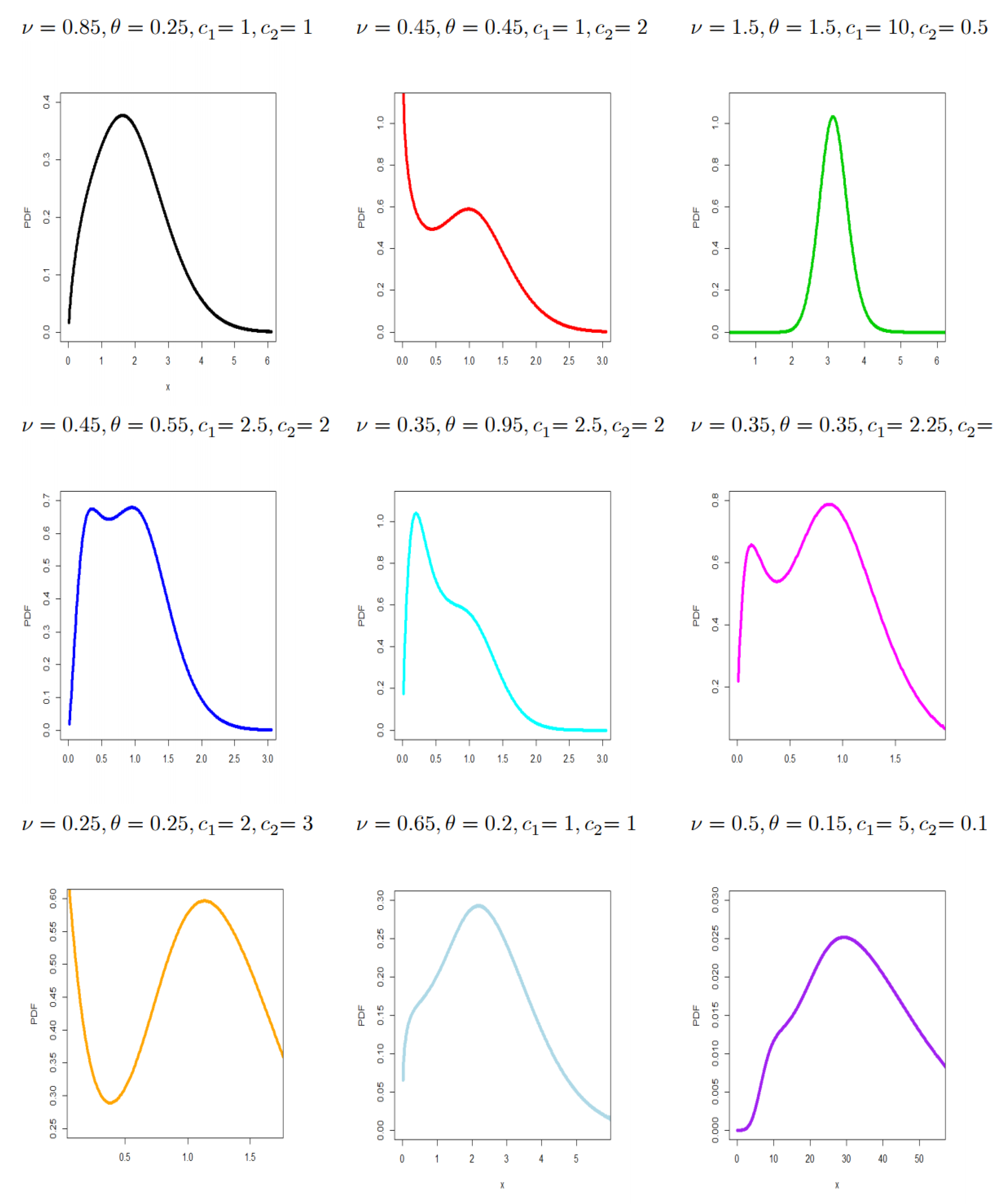
Figure 1. Different plots of the odd Burr BX (OBBX) probability density function (PDF) for selected parameter values.
Symmetry 12 02058 g001
Figure 2. (a) Increasing HRF, (b) Bathtub HRF (U-HRF), (c) J-Shaped HRF (J-HRF), (d) Decreasing HRF, (e) Increasing–Constant–Increasing, (f) Reversed J-HRF, (g) Upside-down (Reversed U-HRF).
Symmetry 12 02058 g002
Figure 3. Three-dimensional skewness plots for some selected values of the parameter θ.
Symmetry 12 02058 g003
Figure 4. Three-dimensional kurtosis plots for some selected values of the parameter θ .
Symmetry 12 02058 g004
Figure 5. Biases (a) and mean squared errors (MSEs) (b) for the parameter ν.
Symmetry 12 02058 g005
Figure 6. Biases (a) and MSEs (b) for the parameter θ.
Symmetry 12 02058 g006
Figure 7. Biases (a) and MSEs (b) for the parameter c1.
Symmetry 12 02058 g007
Figure 8. Biases (a) and MSEs (b) for the parameter c 2 .
Symmetry 12 02058 g008
Figure 9. The TTT, box, quantile-quantile (Q-Q), and NKDE plots for data set I.
Symmetry 12 02058 g009
Figure 10. Estimated probability density function (EPDF), estimated cumulative distribution function (ECDF), probability–probability (P-P), and estimate hazard rate function (EHRF) plots for data set I.
Symmetry 12 02058 g010
Figure 11. The TTT, box, Q-Q, and NKDE plots for data set II.
Symmetry 12 02058 g011
Figure 12. EPDF, ECDF, P-P, and EHRF plots for data set II.
Symmetry 12 02058 g012
Figure 13. The TTT, box, Q-Q, and NKDE plots for data set III.
Symmetry 12 02058 g013
Figure 14. EPDF, ECDF, P-P, and EHRF plots for data set III.
Symmetry 12 02058 g014
Figure 15. The TTT, box, Q-Q, and NKDE plots for data set IV.
Symmetry 12 02058 g015
Figure 16. EPDF, ECDF, P-P, and EHRF plots for data set IV.
Symmetry 12 02058 g016
Table 1. Numerical results for the mean, variance, skewness, kurtosis, and dispersion index for selected parameter values.
ν θ c 1 c 2 E ( W ) V ( W ) S ( W ) K ( W ) DisIx ( W )
121.50.51.39581.06521.00683.63120.7631
1 1.57690.42300.46143.10310.2682
5 1.88550.0271−0.36773.79120.0144
30 1.97530.0008−0.54914.25890.0004
50 1.98280.0003−0.56084.29010.0001
20.50.51.50.52200.07040.95284.22780.1348
1 0.37680.03050.74233.95470.0809
5 0.19300.00700.30532.85430.0365
50 0.07310.00120.39402.56130.0164
100 0.05350.00070.44332.89590.0126
200 0.03890.00040.48664.03050.0095
500 0.02520.00020.22881.86900.0064
1000 0.01818.4 × 10−51.80571.50590.0047
550.51.80.23910.0016−0.46563.40420.0069
1 0.40790.0018−0.64853.86470.0044
5 0.76320.0012−0.72804.13080.0015
50 1.14370.0006−0.828113.31650.0005
100 1.23810.0005−0.69024.02990.0004
500 1.43430.0004−0.67463.98720.0003
1000 1.51110.0004−0.66963.97390.0002
2000 1.58430.0003−0.66573.97870.0002
1510100.31.2 × 10−541.21511.00021.00053,376,320
0.53.20970.0013−0.97604.86690.0004
11.60490.0003−0.98125.32980.0002
20.80248.2 × 10−5−0.97604.86650.0001
30.53503.6 × 10−5−0.97604.85916.82 × 10−5
51.9 × 10−66.5 × 10−7414.9644172,196.50.3333
Table 2. The MLEs (SEs) for data set I.
Distribution Estimates (SEs)
BX(c1;c2)1.1818760.377525
(0.17060)(0.02532)
OLEW(θ;c1;c2)0.159350.73220.765
(0.3712)(1.778)(0.041)
OLBX(θ;c1;c2)1.454060.75430.2379
(0.9018)(0.2530)(0.0317)
BXEW(θ;c1;c2)0.636844.26220.5364
(0.356)(1.757)(0.0997)
PTLW(θ;c1;c2)−5.781754.228650.65801
(1.395)(1.167)(0.039)
MOEW(θ;c1;c2)488.8990.28321261.97
(189.358)(0.013)(351.07)
GamW(θ;c1;c2)2.376970.848093.5344
(0.378)(0.00053)(0.665)
OBBX(ν;θ;c1;c2)1.291023.13310.84480.1906
(0.544)(2.3251)(0.4961)(0.084)
KumW(ν;θ;c1;c2)14.43310.204134.659981.8459
(27.095)(0.042)(17.527)(52.014)
Beta-W(ν;θ;c1;c2)1.360.298134.180211.4956
(1.002)(0.06)(14.838)(6.73)
TrMW(ν;θ;c1;c2)0.272214.6 × 10−60.4685
(0:014)(5.2 × 10⁻⁵)(1.9 × 10⁻⁴)(0.165)
MBW(ν;θ;λ;c1;c2)10.15020.163257.416719.38592.0043
(18.697)(0.019)(14.063)(10.019)(0.662)
MacW(ν;θ;λ;c1;c2)1.94010.30617.68633.638816.7211
(1.011)(0.045)(6.222)(19.994)(9.722)
TrEGW(ν;θ;λ;c1;c2)4.25670.15320.09785.23131173.33
(33.401)(0.017)(0.609)(9.792)(6.999)
Table 3. The Cramér–von Mises (CVM), Anderson–Darling (AD), and Kolmogorov–Smirnov (KS) (p-value) results for data set I.
DistributionCVMADKS (p-Value)
OBBX0.05800.57770.05602 (0.9547)
OLEW0.07230.60860.87572 (<0.001)
OLBX0.07920.59100.37584 (<0.001)
BX0.06900.69160.07981 (0.6584)
BXEW0.07440.64200.06935 (0.8139)
PTLW0.13971.19390.11542 (0.8004)
MOEW0.39954.44770.06170 (0.9064)
GamW0.25531.94890.58482 (0.33119)
KumW0.18521.50590.23917 (0.43651)
Beta-W0.46523.21970.66032 (<0.001)
TrMW0.806511.20470.68989 (<0.001)
MBW0.47173.26560.33902 (<0.001)
MacW0.19861.59060.09243 (0.81193)
TrEGW1.00796.23320.22402 (<0.001)
Table 4. MLEs (SEs) for data set II.
Distribution Estimates (SEs)
BX(c1;c2)0.364130.04763
(0.0373)(0.0039)
W(c1;c2)9.55931.0477
(0.853)(0.068)
OBBX(ν;θ;c1;c2)5.68221.610690.06880.00067
(1.0574)(0.7171)(0.0066)(<0.001)
TrMW(ν;θ;c1;c2)0.12080.89550.00020.2513
(0.024)(0.626)(0.011)(0.407)
MBW(ν;θ;λ;c1;c2)0.15020.163257.416719.38592.0043
(22.437)(0.044)(37.317)(13.49)(0.789)
TrAW(ν;θ;λ;c1;c2)0.11390.97223.09 × 10−51.0065−0.163
(0.032)(0.125)(6.12 × 10⁻³)(0.035)(0.28)
Table 5. The CVM, AD, and KS (p-value) for data set II.
DistributionCVMADKS (p-Value)
OBBX0.03450.20380.04242 (0.9754)
W0.10550.66280.2665 (0.00662)
BX0.47472.78610.35516 (0.0042)
TrMW0.12510.76030.15875 (0.3969)
MBW0.10680.72070.25762 (0.3198)
TrAW0.11290.70330.16872 (0.3376)
Table 6. MLEs (SEs) for data set III.
Distribution Estimates (SEs)
BX(c1;c2)0.936580.00478
(0.1461)(0.0004)
TrBX(θ;c1;c2)0.63281.039170.00417
(0.2453)(0.1445)(0.0005)
OLEW(ν;θ;c1;c2)0.00180.07160.2813
(0.0004)(0.025)(0.009)
OWW(θ;c1;c2)11.15760.08810.457
(4.5449)(0.036)(0.08)
GaEE(θ;c1;c2)2.11382.60060.0083
(1.3288)(0.5597)(0.005)
OBBX(ν;θ;c1;c2)3.248550.405410.29050.0029
(0.8191)(0.1563)(0.039)(0.0003)
Table 7. The CVM, AD, and KS (p-value) for data set III.
DistributionCVMADKS (p-Value)
OBBX0.05490.346010.06916 (0.8812)
BX0.18491.085780.096596 (0.5125)
TrBX0.13520.792590.085663 (0.6662)
OLEW0.25171.475020.999870 (<0.001)
OWW0.44942.476400.658701 (<0.001)
GaEE0.31501.720800.508710 (<0.001)
Table 8. MLEs (SEs) for data set IV.
Distribution Estimates (SEs)
BX(c1;c2)5.485970.9868
(1.1853)(0.0540)
TrBX(θ;c1;c2)−0.655244.786051.04504
(0.19529)(1.2831)(0.0549)
OLBX(θ;c1;c2)0.658312.10190.8429
(0.5112)(1.246)(0.058)
OLEW(θ;c1;c2)0.508782.5341.7122
(0.397)(1.8298)(0.0959)
EW(θ;c1;c2)0.671327.2851.71811
(0.249)(1.707)(0.086)
TrW(θ;c1;c2)−0.50105.14980.6458
(0.2741)(0.6657)(0.0235)
OLLW(θ;c1;c2)0.94396.02560.6159
(0.2689)(1.3478)(0.0164)
OBBX(ν;θ;c1;c2)5.82216.97390.33840.1739
(6.1527)(8.4085)(0.449)(0.2701)
Table 9. The CVM, AD, and KS (p-value) for data set IV.
DistributionCVMADKS (p-Value)
OBBX0.20411.12160.14084 (0.1642)
OLBX0.25571.41540.62469 (<0.001)
TrBX0.47642.61630.19385 (0.01757)
OLEW0.27111.49650.66225 (<0.001)
BX0.55943.07220.21497 (0.00592
EW0.63613.48420.15895 (<0.001)
TrW1.03580.16910.33359 (0.07651)
OLLW1.23640.21940.59001 (0.01543)
Publisher’s Note: MDPI stays neutral with regard to jurisdictional claims in published maps and institutional affiliations.