Exploring Finite-Sized Scale Invariance in Stochastic Variability with Toy Models: The Ornstein–Uhlenbeck Model

Abstract

Stochastic variability is ubiquitous among astrophysical sources. Quantifying stochastic properties of observed time-series or lightcurves, can provide insights into the underlying physical mechanisms driving variability, especially those of the particles that radiate the observed emission. Toy models mimicking cosmic ray transport are particularly useful in providing a means of linking the statistical analyses of observed lightcurves to the physical properties and parameters. Here, we explore a very commonly observed feature; finite sized self-similarity or scale invariance which is a fundamental property of complex, dynamical systems. This is important to the general theme of physics and symmetry. We investigate it through the probability density function of time-varying fluxes arising from a Ornstein–Uhlenbeck Model, as this model provides an excellent description of several time-domain observations of sources like active galactic nuclei. The probability density function approach stems directly from the mathematical definition of self-similarity and is nonparametric. We show that the OU model provides an intuitive description of scale-limited self-similarity and stationary Gaussian distribution while potentially showing a way to link to the underlying cosmic ray transport. This finite size of the scale invariance depends upon the decay time in the OU model.

1. Introduction

Stochastic variations are a central feature of variability in numerous astronomical sources ([1,2,3,4], and references therein) such as active galactic nuclei (AGN), X-ray binaries (XRB), etc. These encode the physical processes driving the particle transport. Traditionally, X-ray observations had decent statistics to attempting quantification of these variations. However, the past two decades have seen an increase in the quality of data across the electromagnetic spectrum. In recent times, there has been an upsurge in efforts to try to quantify this variability with multi-wavelength observations and consequently the driving particle transport. Thus variability of observed electromagnetic radiation and properties of cosmic rays intimately linked to one another. Several properties of lightcurves or observables reveal these links such as the probability density function (PDF), the power spectral density (PSD), etc. The PDF encodes the form or class of the underlying mechanism, for instance, the shape suggests if the processes are additive or multiplicative [1,5]. Moreover, the PSD probes the structure or distribution of the variability timescales [6] Furthermore, two key characteristics of a class of models is stationarity (weak or strong) and presence of self-similarity. Stationarity refers to the fact that statistical properties of the time-series do not change over time. Several astrophysical studies relating to variable sources such as AGN, XRB and even gamma-ray bursts (GRBs) [6,7,8,9,10]. And self-similarity refers to the scale invariance of the time-series. In general, scale invariance relates to features of objects or laws that remain invariant to multiplication by a factor of scales in the system; in complex, dynamical systems this usually refers to scaling of time which is a part of a larger symmetry and is thus important to the theme of this issue. This property has also been investigated for these astronomical sources either from the perspective of the underlying physical model or from the observations in a parametric way [11,12,13,14]. However, both of these properties related to the PDF of the underlying process of which the observed time-series is a realisation. This provides a more direct, nonparametric way of probing self-similarity from the observed lightcurves. The process is strictly stationary, if the joint distribution of each entry or random variable at different times $X_{\mathrm{t}},t\in \mathbf{Z}$ (set of integers) is invariant to time-translation. In practice, and in nature, most processes are only weakly stationary at best, sometimes referred to merely as stationary, i.e., have a constant mean (first moment), finite variance and the autocorrelation depends only on the time lag. The stationary distribution informs us about the class or type of physical mechanism such as additive or multiplicative, properties of the phase space of these random variables, etc. On the other hand, non-stationarity can instruct us about the dynamical evolution of the process. Stochastic variability is often linked to presence of turbulence in the emission regions [14,15,16,17]. Self-similarity is a symptom of turbulence [18]. Indeed, any mechanism capable of producing scale-invariant variations would exhibit self-similarity in the lightcurves provided, it is the dominant mechanism at those scales [19]. For instance, cascades can demonstrate scale invariance [20,21]. Self-similarity even in a specific range of time-scales is highly instructive. It can give clues into the transition to turbulent regimes [22]. Presence of self-similarity has been studied in several sources. Here we attempt to characterize certain symptoms of self-similar features, using toy models and simulations of stochastic processes, particularly through the probability density function. In particular, we look at the Ornstein–Uhlenbeck or OU process that has had success in modeling stochastic variability in AGN.

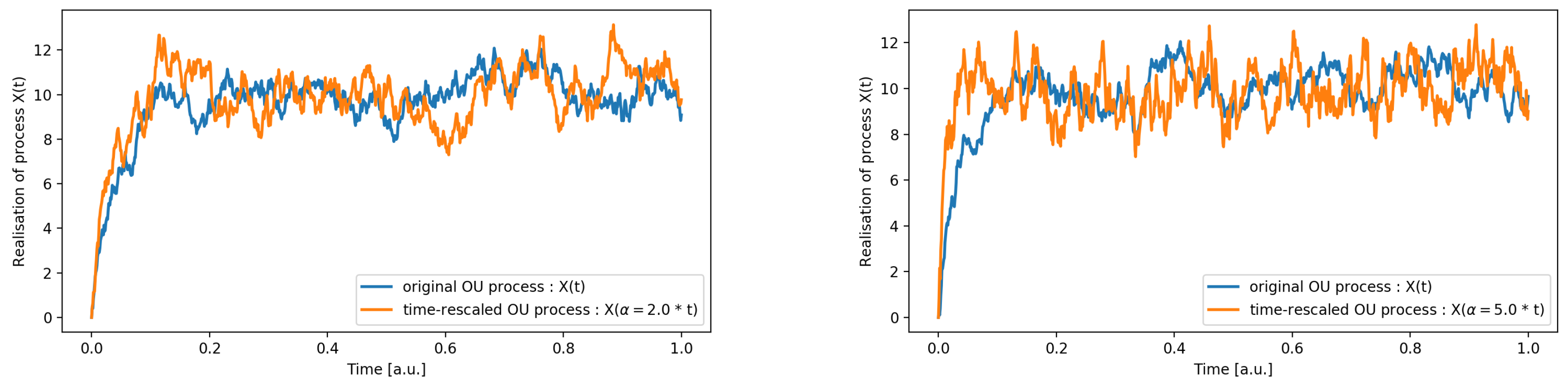
2. Stochastic Processes: Ornstein–Uhlenbeck Model for Transport

Stochastic processes have been used in several fields to model noisy time-series. Astrophysics is no different. Numerous sources show variability that is noisy not due to observational methods, but stochasticity inherent to the physical processes. Quantifying the stochasticity in the observations, we can learn about the underlying particle transport or even the accretion disk model [23]. Sources like AGN, quasars and blazars have been modelled successfully by stochastic models like the OU process ([3,24] and the references therein). Unlike Brownian motion, it has the advantage of a stationary, Gaussian distribution. However, the Brownian process has the property of self-similarity. It can be shown that Ornstein–Uhlenbeck process can be used to provide a finite-sized scale invariant process from a Brownian process using the Lamperti transform [25]. This essentially means that the resulting process will be scale invariant in bounded ranges of scales and amplitudes. This is what we expect to encounter practically in actual observations as scale invariance cannot physically last over an infinite range of scales. Here, we attempt to explore a toy model of underlying particle transport that could provide a source of stochasticity in the radiative output. Consider the continuity equation which describes the temporal evolution of a population of electrons in a blob. The number of electrons, N as a function of their Lorentz factor $\gamma$ and time t is given by [26,27,28]

$$\begin{array}{c}\hfill \frac{\partial N(\gamma ,t)}{\partial t}+\frac{\partial \dot{\gamma }N(\gamma ,t)}{\partial \gamma }+\frac{N(\gamma ,t)}{t_{\mathrm{esc}}(\gamma ,t)}=Q(\gamma ,t)\end{array}$$

(1)

where $\dot{\gamma }$ is the energy loss rate, $t_{\mathrm{esc}}(\gamma ,t)$ is the escape timescale of the electrons, and $Q(\gamma ,t)$ is the source term, which in general depend on $\gamma$ and t. Initially assuming no radiative losses and only escape, we get

$$\begin{array}{c}\hfill e^{t/t_{\mathrm{esc}}}\frac{\partial N}{\partial t}+e^{t/t_{\mathrm{esc}}}\frac{N}{t_{\mathrm{esc}}}=e^{t/t_{\mathrm{esc}}}Q\end{array}$$

(2)

Assuming that the escape time is a constant, and the source term Q is stochastic in nature and given by $Qdt=AdW\left(t\right)$ we can write the solution as

$$\begin{array}{ccc}\hfill N\left(t\right)& =& N\left(0\right)e^{-t/t_{\mathrm{esc}}}+A{\int }_0^t{e}^{-(t-s)/t_{\mathrm{esc}}}dW\left(s\right)\hfill \end{array}$$

(3)

Now, in case we include radiative losses, typically synchrotron and inverse-Compton, we can write this term as

$$\begin{array}{c}\hfill \dot{\gamma }=B{\gamma }^2\end{array}$$

(4)

where B represents the coefficient of the loss rate, independent of $\gamma$ and t, which for synchrotron and Compton losses depends on energy density of the magnetic field and the target photon or radiation fields. Equation (4) holds true for the Thomson limit for Compton losses. Then, in Equation (3) we replace $1/t_{\mathrm{esc}}$ by $Bf\left(\gamma \right)+1/t_{\mathrm{esc}}$, where f is a function giving us

$$\begin{array}{ccc}\hfill N\left(t\right)& =& N\left(0\right)e^{-\left(Bf\left(\gamma \right)+1/t_{\mathrm{esc}}\right)t}+A{\int }_0^t{e}^{-\left(Bf\left(\gamma \right)+1/t_{\mathrm{esc}}\right)(t-s)}dW\left(s\right)\hfill \end{array}$$

(5)

Thus, the particle (in this case electron) evolution can be cast into an OU process under these assumptions. Here, are some notable features of such a particle or cosmic ray model. Note that for long enough times ($t\to \infty$), the distribution tends to a stationary Gaussian distribution. Moreover, unlike in a purely Brownian motion, N tends to “drift” back to the mean value owing to the first term in Equation (5). This is sometimes referred to as mean reverting (It is referred to in this way, especially in the domain of finance, where it is used successfully to model stock prices.). Critically, this allows the value of the random variable (N or X) to remain bounded. The PSD of an OU process is of the form of a Lorentzian or $PSD\left(\omega \right)\sim 1/(c^2+{\omega }^2)$ where the (angular) frequency $\omega =1/\left(2\pi t\right)$. So while on long timescales, it tends to Gaussian white noise, at shorter timescales it tends to red noise. In addition to these, a pure Brownian motion is a self-similar stochastic process. This scale invariance is present in the statistical, temporal properties including the $1/w^2$ behavior of the PSD. However, there are physical limits to the range of variables, and this limits the range of scale invariance as well. A physically motivated model for stochastic variability state stemming from turbulent or cascade type process must have the ability to account for self-similarity observed in a limited range as well as a stationary distribution. Mathematically speaking, this finite range scale-invariance with a stationary distribution can be achieved by means of a Lamperti transformation for details of which readers are referred to Amblard et al. [25]. The essential point is that the OU process allows for not only a stationary, Gaussian distribution suitable for a number of observations, but also the capacity to model self-similarity in a physical, range-limited sense.

Assuming that the time-travel effects or indeed the radiative losses do not have significant stochasticity of their own, the stochasticity in the source or injection term will be the principle influence on variability in the emitted radiation. This includes the assumption relativistic transformation from the emission frame (say jet frame) to the observe frame also does not have a stochastic component. Under this assumption, the observed stochastic properties of the lightcurve, $X\left(t\right)$ correspond to the statistics of the source term, $Q\left(t\right)$. Thus, the exponential trend in the electron number with time, is randomly perturbed or modulated by the source term. These random fluctuations are imprinted in the statistical properties of the lightcurves, including in its distribution. Thus, any properties of the time-series or its distribution can be traced back to the source of the underlying cosmic ray particles—electrons in this model. Now, from the loss rate of a single electron, and the distribution of electrons that is time-dependent we can get the photon emissivity as

$$\begin{array}{c}\hfill j_{\nu }\propto \int \langle P_{loss,\nu }\rangle n_{\mathrm{e}}\left(\gamma \right)d\gamma \end{array}$$

(6)

where $n_{\mathrm{e}}\left(\gamma \right)$ is the number density of electrons From this it is clear that the stochastic properties of the injected spectrum is transferred to the photon emissivity and therefore the flux. Therefore, the mean emissivity is the product of the average loss rate $\langle P_{loss,\nu }\rangle$ and the number density of electrons $n_{\mathrm{e}}$. For long enough times, i.e., $t\gg t_{\mathrm{acc}}$ and $t\gg \frac{1}{\nu }$, the time dependence and therefore stochasticity (time domain) of the photon emissivity, $j_{\nu }\left(t\right)$ tracks that of the number density, $n_{\mathrm{e}}(\gamma ,t)$. This assumes that the loss rates themselves have no competing stochasticity such as in the magnetic field or indeed in the target radiation fields for inverse-Compton emission.

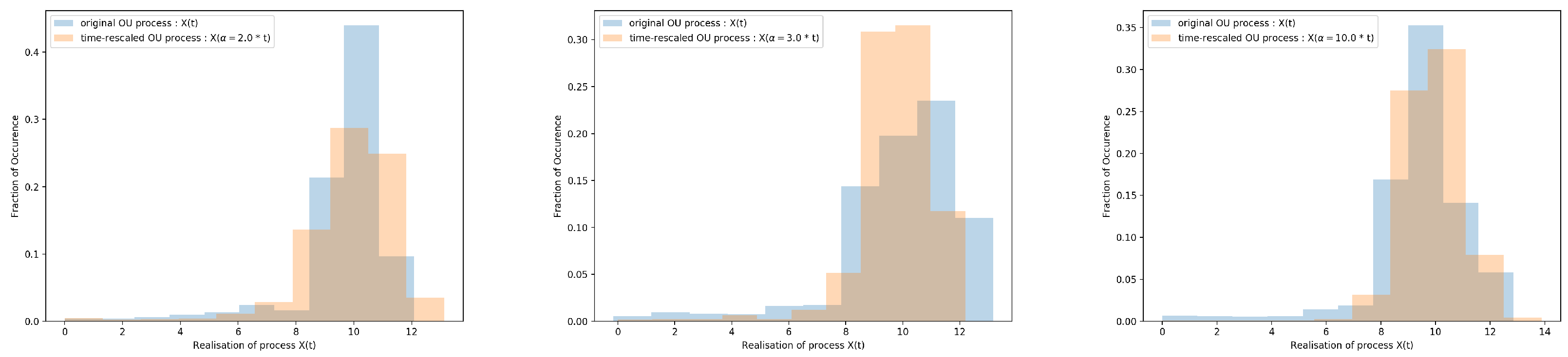
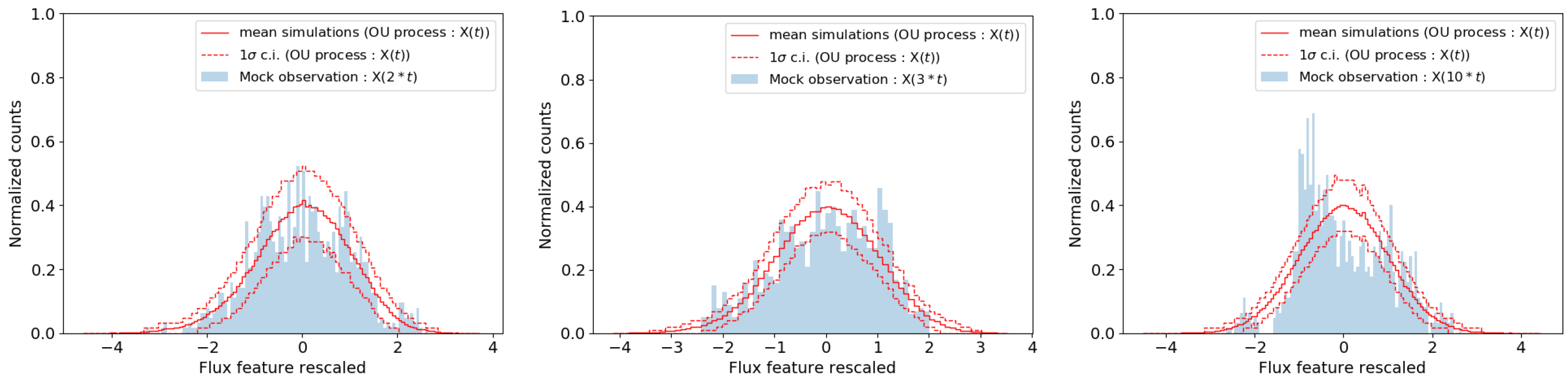
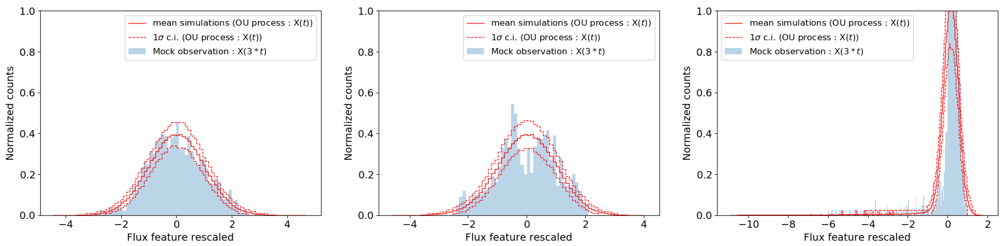
3. Testing Stochastic Properties with OU Simulations

Self-similarity is a crucial feature that can aide in identifying class of physical mechanisms at play. As defined in Tudor [19], a stochastic process $X_{\mathrm{t}}$ is said to be self-similar, if there exists a constant H, such that for every real number $\alpha >0$, $X_{\alpha \ast t}$ and ${\alpha }^H{X}_{\mathrm{t}}$ have the same distribution. As explained before, establishing scale invariance within a limited range of time-scales is quite useful in pinning down models. Here, we wish to provide a set of ways of quantifying this self-similarity from data. In order to demonstrate a proof-of-principle, we will use mock observations simulated using the OU process. This is a model that has successfully captured the stochastic of variable sources as quasars [4]. It is appropriate for processes with a Gaussian distribution. This is ideally suited for our experiments with toy models. We perform certain scaling tests on these time-series or lightcurves generated by this process to quantify self-similarity or scale invariance. Realizations of these scaled and unscaled time-series appear as shown in the Figure 1. These are time-series or mock lightcurves simulated for scaling factor $\alpha =2$ and 5, respectively. Very clearly, one can observe that the features in the $\alpha =5$ lightcurve appeared squeezed within a shorter interval along the time axis relative to $\alpha =2$. This shows the scaling but any hints of invariance requires investigation into statistical properties. For this we compare the distributions of the original and scaled processes.

As stated in the previous section, we test the scaling properties of the OU process simulating realizations. The stochastic differential equation for the OU process is given by

$$dX\left(t\right)=-\frac{X\left(t\right)-\mu }{\tau }dt+\sigma \sqrt{\frac{2}{\tau }}dW$$

(7)

Note that this process has a Gaussian distribution and is thus appropriate for only those scenarios, which are commonly observed. Interpreting the random variable, X as the emissivity without loss of generality, the mean $\mu$ is given by the temporal average of Equation (6). Of course, the values of these parameters are estimated from observations. Moreover, note that for distant sources like AGN, the cosmological time dilation factor, (1 + z) where z is the redshift is obviously independent of time and can be absorbed in $\sigma \to \sqrt{(1+z)}\sigma$ [3]; while this factor is $>1$, the scaled sigma can still be $<1$. The simulations for this model are generated by the discretization as

$$X_{\mathrm{n}+1}=X_{\mathrm{n}}+dt\left(-\frac{X_{\mathrm{n}}-\mu }{\tau }\right)+\sigma \sqrt{\frac{2}{\tau }}\sqrt{dt}\xi$$

(8)

where $t=n\ast dt$ and $\xi \sim N(0,1)$ is simply a random Gaussian variable with mean 0 and variance 1. The presence of $\sqrt{dt}$ in the normalization is essentially because in a Brownian type motion, the increments in the random variable scale as $\Delta X{\left(t\right)}^2\sim \Delta t$. Now, we test the scale invariance by introducing the temporal scaling factor $\alpha$. Practically this translates to transforming $dt\to \alpha dt$ which obviously also transforms, $t\to \alpha t$. This scale invariance can be quantified in terms of the Hurst index, H for self-similarity introduced earlier in Section 3. For details of ways of estimating H, the reader is referred to the works ([29,30], and references therein). In this work, we focus on the comparing the distributions of the scaled and unscaled variables.

The strictest mathematical condition for self-similarity is expressed in terms of the distribution of the random process. A stochastic process X(t) (or typically represented in mathematical texts as ${\left(X_{\mathrm{t}}\right)}_{t\ge 0}$) is self-similar if there exists a real number, H, such that distributions of processes $X\left(\alpha t\right)$ and ${\alpha }^{H}X\left(t\right)$ are the same. In other words, the distribution of PDF is invariant under scaling of time. We put this to test explicitly for the OU process. Once again, we simulate mock observations of the OU process $X\left(t\right)$ generated using the discretized stochastic differential equation for the OU process in Equation (8).

We determine histograms of the resulting scaled time-series for several values of $\alpha$; we show the comparisons between $X\left(t\right)$ and $X\left(\alpha t\right)$ for the values $\alpha =2,3$ and 10 in Figure 2. For each case, the histogram of the single realization of $X\left(t\right)$ and $X\left(\alpha t\right)$ look quite similar. To robustly evaluate the significance of this similarity we simulate an ensemble of time-series and compute the confidence intervals of for each bin as detailed in [31,32]. We simulate with $\alpha \ne 1$ and then use the original time-series ($X\left(t\right)$ or $\alpha =1$) as the mock observation. Comparisons for $\alpha =2,3$ and 10 simulations are shown in Figure 3. The OU process is simulated with the discrete scheme as stated in Equation (8). Once again, the time-series are simulated with a mean, $\mu =3.0$, standard deviation, $\sigma =1.0$ and a relaxation time, $\tau =0.1$. Following that, for evaluating confidence intervals of histogram bins from simulations, we rescale the flux values to have a mean 0 and standard deviation of 1. The red-dashed histograms represent $1-\sigma$ confidence intervals for each bins. The figure shows that the distributions for $\alpha =2$ and even $\alpha =3$, $X\left(t\right)$ and $X\left(\alpha t\right)$ are compatible to within statistical uncertainties. Performing the Kolmogorov–Smirnov test comparing simulations to the observations, we get p-values of 0.31 and 0.28 at the 84th percentile for $\alpha =2$ and 3, respectively, showing that they are likely drawn from the same distribution. For $\alpha =10$, we start to see deviations between the rescaled simulations ($X(\alpha \ast t)$) and the mock observation ($X\left(t\right)$) with p-value of 0.008 for the KS test at the 84th percentile. This suggests that for lower $\alpha$ values while individual realizations of time-series themselves may show deviations from expected correlations, statistical comparisons with the ensemble shows that they belong to the same distribution. However, the evidence of such scale invariance weakens as we go to larger $\alpha$ values as seen in the case $\alpha =10$. We know that in the OU model $\tau$ represents the decay or time; in other words the time taken for the noisy fluctuations to dissipate. It also marks the timescale at which the we see the transition from red noise to white noise behavior. We see that on varying this decay time, $\tau =0.5,0.1,0.05,0.01$ keeping the mean fixed at $\mu =3.0$ and standard deviation at $\sigma =1.0$, the p-values improve with decreasing $\tau$ as $1.2\times {10}^{-4},0.31,0.36,0.91$ respectively, for the $\alpha =3$ case. This is shown in the Figure 4. We see in this particular OU model, that within an order of magnitude of the scaling factor, $\alpha$, there are deviations from the scale invariance. Noting that the scale-invariance comes from the Brownian source term, from Equation (5), we see that the time-scaling parameter $\alpha$, can be related to the overall scaling or normalization of the loss terms in the continuity equation. Specifically, $t\to \alpha t$ and $dW\to {\alpha }^{1/2}dW$ could be reinterpreted in terms of $\left(Bf\left(\gamma \right)+1/t_{\mathrm{esc}}\right)\to {\alpha }^{3\eta /2}\left(Bf\left(\gamma \right)+1/t_{\mathrm{esc}}\right)$ keeping the distribution of the stochastic term and N fixed, where $\eta$ depends on the scale invariance parameter.

4. Discussions and Conclusions

The scaling properties of time-domain observations are powerful indicators of the underlying physical mechanisms. Models of cosmic ray transport such as turbulence or cascades can cause scale invariant features to appear in the observations. Of particular interest here are such features in the time domain. Self-similarity in time-series or lightcurves is therefore a key probe of the dynamics of the physical mechanism. Furthermore, this feature is fundamentally linked to the distribution of the observable which in the case of stochastic lightcurves is simply the flux. In this work we attempt to quantify scale invariance or self-similarity via probability density function of the time-rescaled and the original time-series. This is a different approach from estimating the Hurst coefficient (see in [33] and the references therein) in different ways such as wavelet transform, PSD analysis, $R/S$ analysis, etc. detailed in Serinaldi [30]. This approach is more directly derived from the basic mathematical definition of self-similar stochastic processes and is nonparametric. On the other hand, it requires good quality observations capable of constraining the PDF. In order to do this, we perform experiments with the OU process as a toy model as this has successfully been applied to stochastic variability in a number of sources. We see finite-sized scale invariance for the OU process, is valid only within a limited range of time-scaling parameter $\alpha$. This range also depends upon the decay time, $\tau$. Our results suggest that for shorter decay times, the finite-sized scale invariance effect is stronger and lasts more than an order-of-magnitude. From the stochastic equation representing the evolution of the OU process for transport with escape and radiative losses (synchrotron and inverse-Compton in Thomson regime), we find that $\alpha$ can parameterize the overall amplitude of these losses for localized or one-zone models. Thus, from the range of values of scale invariance, we can put constraints on the overall normalization of the losses. This assumes that the propagation of the radiation in space (time-travel effects, spatial turbulence in jets, etc.) does not have a significant contribution; if that were the case, the $\alpha$ parameter would have a more complex relationship with the physical parameters. This would give us some insights into flares where one-zone models are applicable. In general, dissecting the self-similar features can potentially probe properties of underlying turbulent or cascade type models (see, e.g., in [14,34,35]). Making such connections is beyond the scope of this work. Moreover, this model is limited to the Gaussian distributions; lognormal distributions can also be modeled if we apply it to the log-values of the random variable. However, more general distributions have been found in nature. Furthermore, extensions to this model are needed to model those and will be explored in future work. Here we show, using the probability density function, there is a direct way of establishing scale invariance, even when it is scale limited. Moreover, by doing so, we have a way of connecting the observed stochasticity and its features to the physical parameters of the cosmic ray transport model.

References

1. Lyubarskii, Y.E. Flicker noise in accretion discs. Mon. Not. R. Astron. Soc. 1997, 292, 679–685. [Google Scholar] [CrossRef] [Green Version]
2. Uttley, P.; McHardy, I.M.; Vaughan, S. Non-linear X-ray variability in X-ray binaries and active galaxies. Mon. Not. R. Astron. Soc. 2005, 359, 345–362. [Google Scholar] [CrossRef] [Green Version]
3. Kelly, B.C.; Bechtold, J.; Siemiginowska, A. Are the Variations in Quasar Optical Flux Driven by Thermal Fluctuations? Astrophys. J. 2009, 698, 895–910. [Google Scholar] [CrossRef]
4. Sobolewska, M.A.; Siemiginowska, A.; Kelly, B.C.; Nalewajko, K. Stochastic Modeling of the Fermi/LAT γ-Ray Blazar Variability. Astrophys. J. 2014, 786, 143. [Google Scholar] [CrossRef] [Green Version]
5. Vaughan, S.; Uttley, P. Studying accreting black holes and neutron stars with time series: Beyond the power spectrum. arXiv 2008, arXiv:0802.0391. [Google Scholar]
6. Vaughan, S.; Edelson, R.; Warwick, R.S.; Uttley, P. On characterizing the variability properties of X-ray light curves from active galaxies. Mon. Not. R. Astron. Soc. 2003, 345, 1271–1284. [Google Scholar] [CrossRef]
7. Scargle, J.D. Studies in astronomical time series analysis. I—Modeling random processes in the time domain. Astrophys. J. Suppl. Ser. 1981, 45, 1–71. [Google Scholar] [CrossRef]
8. Bhatt, N.; Bhattacharyya, S. Time evolution of the probability density function of a gamma-ray burst: A possible indication of the turbulent origin of gamma-ray bursts. Mon. Not. R. Astron. Soc. 2012, 420, 1706–1713. [Google Scholar] [CrossRef]
9. Bhattacharyya, S.; Ghosh, R.; Chatterjee, R.; Das, N. Blazar Variability: A Study of Nonstationarity and the Flux-Rms Relation. Astrophys. J. 2020, 897, 25. [Google Scholar] [CrossRef]
10. Budai, A.; Raffai, P.; Borgulya, B.; Dawes, B.A.; Szeifert, G.; Varga, V. A statistical method to detect non-stationarities of gamma-ray burst jets. Mon. Not. R. Astron. Soc. 2020, 491, 1391–1397. [Google Scholar] [CrossRef]
11. McHardy, I.; Czerny, B. Fractal X-ray time variability and spectral invariance of the Seyfert galaxy NGC5506. Nature 1987, 325, 696–698. [Google Scholar] [CrossRef]
12. Georganopoulos, M.; Marscher, A.P. Self-Similarity and Observed Properties in Blazars. In Proceedings of the Astronomical Society of the Pacific Conference Series, Turku, Finland, 22–26 June 1999; p. 359. [Google Scholar]
13. An, T.; Baan, W.A. The Dynamic Evolution of Young Extragalactic Radio Sources. Astrophys. J. 2012, 760, 77. [Google Scholar] [CrossRef] [Green Version]
14. Marscher, A.P. Turbulent, Extreme Multi-zone Model for Simulating Flux and Polarization Variability in Blazars. Astrophys. J. 2014, 780, 87. [Google Scholar] [CrossRef]
15. Blandford, R.D.; McKee, C.F. Fluid dynamics of relativistic blast waves. Phys. Fluids 1976, 19, 1130–1138. [Google Scholar] [CrossRef]
16. Falle, S.A.E.G. Self-similar jets. Mon. Not. R. Astron. Soc. 1991, 250, 581–596. [Google Scholar] [CrossRef]
17. Riordan, M.O.; Pe’er, A.; McKinney, J.C. Blazar Variability from Turbulence in Jets Launched by Magnetically Arrested Accretion Flows. Astrophys. J. 2017, 843, 81. [Google Scholar] [CrossRef] [Green Version]
18. Klewicki, J.C. Self-similar mean dynamics in turbulent wall flows. J. Fluid Mech. 2013, 718, 596–621. [Google Scholar] [CrossRef]
19. Tudor, C. Analysis of Variations for Self-Similar Processes: A Stochastic Calculus Approach; Springer: Cham, Switzerland, 2013. [Google Scholar] [CrossRef]
20. Mandelbrot, B.B. Intermittent turbulence in self-similar cascades: Divergence of high moments and dimension of the carrier. J. Fluid Mech. 1974, 62, 331–358. [Google Scholar] [CrossRef]
21. Zrake, J. Inverse Cascade of Nonhelical Magnetic Turbulence in a Relativistic Fluid. Astrophys. J. Lett. 2014, 794, L26. [Google Scholar] [CrossRef] [Green Version]
22. Manneville, P. Intermittency, self-similarity and 1/f spectrum in dissipative dynamical systems. J. Phys. 1980, 41, 1235–1243. [Google Scholar] [CrossRef]
23. Alston, W.N. Non-stationary variability in accreting compact objects. Mon. Not. R. Astron. Soc. 2019, 485, 260–265. [Google Scholar] [CrossRef]
24. Takata, T.; Mukuta, Y.; Mizumoto, Y. Modeling the Variability of Active Galactic Nuclei by an Infinite Mixture of Ornstein–Uhlenbeck (OU) Processes. Astrophys. J. 2018, 869, 178. [Google Scholar] [CrossRef] [Green Version]
25. Amblard, P.O.; Borgnat, P.; Flandrin, P. Stochastic processes with finite size scale invariance. In Proceedings of the Noise in Complex Systems and Stochastic Dynamics, Santa Fe, NM, USA, 2–4 June 2003. [Google Scholar] [CrossRef]
26. Chiaberge, M.; Ghisellini, G. Rapid variability in the synchrotron self-Compton model for blazars. Mon. Not. R. Astron. Soc. 1999, 306, 551–560. [Google Scholar] [CrossRef] [Green Version]
27. Böttcher, M.; Chiang, J. X-Ray Spectral Variability Signatures of Flares in BL Lacertae Objects. Astrophys. J. 2002, 581, 127–142. [Google Scholar] [CrossRef]
28. Finke, J.D.; Becker, P.A. Fourier Analysis of Blazar Variability. Astrophys. J. 2014, 791, 21. [Google Scholar] [CrossRef] [Green Version]
29. Gao, J.B.; Cao, Y.; Lee, J.M. Principal component analysis of 1/ fα noise. Phys. Lett. 2003, 314, 392–400. [Google Scholar] [CrossRef]
30. Serinaldi, F. Use and misuse of some Hurst parameter estimators applied to stationary and non-stationary financial time series. Phys. Stat. Mech. Its Appl. 2010, 389, 2770–2781. [Google Scholar] [CrossRef]
31. Romoli, C.; Chakraborty, N.; Dorner, D.; Taylor, A.; Blank, M. Flux Distribution of Gamma-Ray Emission in Blazars: The Example of Mrk 501. Galaxies 2018, 6, 135. [Google Scholar] [CrossRef] [Green Version]
32. Chakraborty, N. Investigating Multiwavelength Lognormality with Simulations—Case of Mrk 421. Galaxies 2020, 8, 7. [Google Scholar] [CrossRef] [Green Version]
33. Tarnopolski, M.; Żywucka, N.; Marchenko, V.; Pascual-Granado, J. A Comprehensive Power Spectral Density Analysis of Astronomical Time Series. I. The Fermi-LAT Gamma-Ray Light Curves of Selected Blazars. Astrophys. J. Suppl. Ser. 2020, 250, 1. [Google Scholar] [CrossRef]
34. Boffetta, G.; Carbone, V.; Giuliani, P.; Veltri, P.; Vulpiani, A. Power Laws in Solar Flares: Self-Organized Criticality or Turbulence? Phys. Rev. Lett. 1999, 83, 4662–4665. [Google Scholar] [CrossRef] [Green Version]
35. Cafiero, G.; Vassilicos, J.C. Non-equilibrium turbulence scalings and self-similarity in turbulent planar jets. Proc. R. Soc. Math. Phys. Eng. Sci. 2019, 475, 20190038. [Google Scholar] [CrossRef] [Green Version]
Figure 1. The figure shows realizations of the Ornstein Uhlenbeck process for the original time-series X t (blue) and the rescaled one X ff t (orange) for α = 2 and α = 5 , respectively.
Symmetry 12 01927 g001
Figure 2. The histograms of the random processes or time-series, X ( t ) (blue) and X ( α t ) (light orange) for α = 2 , 3 , 10 . We see that histograms for both the original and scaled processes appear to be similar.
Symmetry 12 01927 g002
Figure 3. The histogram of the original OU time-series, X ( t ) with μ = 3.0 , σ = 1.0 and τ = 0.1 (blue gray) which is perfectly compatible with simulations of X ( α t ) (red) for α = 2 , 3 , 10 . This shows that statistically the scaling of time leaves the distribution compatible with the original one for α = 2 and α = 3 , but shows deviations for α = 10 .
Symmetry 12 01927 g003
Figure 4. The figure shows the histogram of the original OU time-series, X ( t ) with μ = 3.0 , σ = 1.0 and values of τ = 0.01 (Left), τ = 0.05 (Center) and τ = 0.5 (Right) (blue grey) compared with simulations of X ( α t ) (red) for α = 3 . It shows that compatibility improves with decreasing decay times, τ .
Symmetry 12 01927 g004
Publisher’s Note: MDPI stays neutral with regard to jurisdictional claims in published maps and institutional affiliations.