1. Introduction
Nowadays, higher education is considered a service industry, and it is expected to meet the expectations of stakeholders by re-evaluating the education system [
1,
2]. The importance of student feedback is acknowledged by universities. In particular, student comments are regarded as an effective way to discuss learning issues online. Comments, posted by students on forums, provide valuable information when it comes to teaching and learning. The purpose of this work is to automatically extract keywords from student comments to enhance teaching quality. In fact, topic keywords have been used for text summarization, terms index, classification, filtering, opinion mining, and topic detection [
3,
4,
5,
6,
7,
8]. Topic keywords are usually extracted by domain experts. It is an extremely time-consuming, complex work. In contrast, automatic extraction is very efficient. Automatic topic keyword extraction refers to the automatic selection of important and topical words from the content [
9]. However, different approaches have different performances. These approaches are performed to discover which approach performs best in extracting topic keywords automatically from a particular type of dataset.
A topic keyword, extracted from a document, is a semantic generalization of a paragraph or document, and an accurate description of the document’s content [
10,
11,
12]. In other words, a topic keyword can be regarded as the category label of a generalized paragraph or document by using its keywords as the features. The extraction accuracy of topic keywords affects many tasks in natural language processing (NLP) and information retrieval (IR), such as text classification, text summarization, opinion mining, and text indexing [
13]. Different approaches are used to automatically extract the keywords from the text to improve performance.
However, there are challenges concerning how to improve the accuracy of topic keyword extraction. With big data growing, unstructured data are everywhere on the internet. Moreover, there are often many language fragments or documents without topic keywords. This makes it even more difficult to process and analyze them. There are many methods and various applications for keyword extraction. The accuracy of topic keyword extraction must continuously improve.
The problem of this work is to extract the topic keywords from student comments, and predict the topic for a new given comment by using supervised learning. As a category label, each of the topic keywords, such as assignments, online meeting, and topic 2 is the summary of semantically related keywords in a group of comments. A feature vector consisting of the keywords, or their embedding in each comment is used to predict its corresponding category label. In this paper, we compare several approaches to extract topic keywords from student comments. Specifically, the compared machine learning algorithms are Naïve Bayes, logistic regression (LogR), support vector machine (SVM), convolutional neural networks (CNN), and Att-LSTM. The performance of the first three algorithms relies heavily on manually selected features, while the last two algorithms are capable of automatically extracting discriminative features from the comments in the training data.
The contributions of this paper are as follows: (1) we compare the performance of different typical algorithms against the subject database in terms of several evaluation metrics; (2) we visualize the keywords and their similarities in the dataset; and (3) we evaluate the performance of the algorithms by using metrics, with visualization of the results of algorithms as further validation.
The paper is the extended version of the conference paper [
14]. New content includes a more thorough literature review, and more comprehensive methodology descriptions, algorithm comparisons, and analysis results. The rest of this paper is organized as follows. In the following section, we review related work.
Section 3 presents the compared algorithms, followed by the experiments in
Section 4.
Section 5 describes the visualization results and
Section 6 concludes this paper.
2. Related Work
Overall, keyword extraction approaches can be classified into simple statistical approaches, linguistic approaches, machine learning approaches, and other approaches [
15].
Simple statistical approaches do not require training. They generate topic keywords from candidates based on analysis and statistics of text and calculation of word frequency, probabilities, and other features extracting, such as term frequency inverse document frequency (TF-IDF) [
16], word frequency [
17], N-Gram [
18], and word occurrences [
19]. Most statistical approaches are used by unsupervised learning approaches. The mechanism of the methods assigns weights to each word and calculates them by feature detection.
Based on the linguistic features of words, sentences, and entire documents, linguistic approaches include words [
20], the syntax [
21], and context to analyze [
22,
23] and find topic keywords in the documents [
15]. For linguistic approaches, the analysis is very complex, requiring some linguistic skills.
Machine learning approaches are classified into four main types of learning: supervised learning [
24], semi-supervised learning, unsupervised learning [
25], and reinforcement learning. With the development of machine learning and NLP, and the various application fields, different machine learning methods for topic keyword extraction have been successfully applied. As supervised learning, these methods use existing datasets to conduct a lot of training on the algorithm model and adjust the parameters in a way that high accuracy of the predictions can be achieved. For topic keyword extraction, supervised learning is, however, commonly used. For this work, the compared algorithms extract the topic keywords from the text based on the existing algorithms. In particular, we choose Naïve Bayes (NB) [
26], logistic regression [
27], SVM [
28], and two deep learning algorithms as approaches for the keyword extraction.
As machine learning methods, which are based on artificial neural networks, deep learning has achieved high performance in many areas. In this work, two types of deep learning algorithms are used for topic keyword extraction. Deep learning [
29] constructs multiple layers of neural networks. It achieved great success recently, in many areas, by automatically extracting keywords from raw text. The domain includes various tasks in natural language processing, such as language modeling, machine translation, and many others. Some researchers used the recurrent neural network (RNN) to extract topic keywords from different scale texts. Zhang et al. used RNN, LSTM, and others to compare the approaches of extracting topic keywords from Twitter datasets. Their deep learning methods achieved good performances.
Long Short-Term Memory (LSTM), a particular type of RNN, achieved a good performance in topic keyword extraction from many domain contents for different purposes. It differs from traditional RNN, and is well suited to classify, process, and predict text problems. Moreover, CNNs perform greatly in image recognition. Recently, CNNs have been applied to text classification—performing very well—but the results are always affected by the quality of the datasets. In this work, these two algorithms will be applied to the student comments and their performances will be compared.
Other keyword extraction approaches use some of the methods above combined with special features to obtain the topic keywords from the text. These features, for example, can include word length, text formatting, and word position [
30].
In the following, we review the algorithms used in our experiments.
Keyword extraction can also be thought of as binary text classification. In other words, it determines whether a particular candidate keyword is the exacted topic keyword or not. Based on these binary approaches, topic keywords can also be used for other applications, such as browsing interfaces [
31], thesaurus construction [
32], document classification, and clustering [
33,
34].
2.1. Naïve Bayes
As a simple, effective, and well-known classifier, Naïve Bayes (NB) uses the Bayes probability theory and statistics, with good performance, on high dimensionality of input [
35].
Kohavi [
36] showed that the performance of NB was not as good as decision trees on the large datasets, so the author combined NB into a decision tree called NB-Tree. In other words, this approach integrated benefits from both the Naïve Bayesian classifier and decision tree classifier. As such, it performed better than each of its components, especially for large datasets. In particular, the decision tree nodes used univariates as regular decision-trees and the leaves as Naïve-Bayes classifiers.
Yasin et al. [
37] used a Naïve Bayesian approach as a classifier to extract the topic keywords from the text with supervised learning. In their work, they assumed that the keyword features were normally distributed, independently. The approach extracted topic keywords from the testing set with the knowledge of training gained. The features were used by TF-IDF scores, word distances, paragraph keywords, and sentences from the text.
In the text classification by Kim et al. [
38], NB was regarded as the parameter estimation process, resulting in the lower accuracy of classification. They proposed per-document text normalization and feature weighting methods to improve its performance. For the classification task, the NB classifier showed a great performance. The Poisson NB was weight-enhancing, by assuming that the input text was processed by the multivariate Poisson model.
2.2. Logistic Regression
As a statistical model, LogR is the core method used by a logistic function. It is also called a sigmoid function, the shape of which is like an s-shape, especially performing best in binary classification. However, it is easy to extend for a multi-class task. It uses probabilities for the classification problem with two outcomes, such as diagnosis of spam emails. It predicts whether or not an email is a spam by using the different features of the email. LogR is used for relationship analysis in dichotomous issues. For text classification, LogR is widely applied to the binary task because the output of LogR probability is between 0.0 and 1.0 [
39]. LogR performs well on these tasks, which predict the resultant presence or absence of a feature of the outcome by the Logistic function.
Tsien et al. [
40] used a classification tree and LogR to diagnose myocardial infarction. They compared the performance of the Kennedy LogR against the Edinburgh and Sheffield dataset, with improving ROC up to 94.3% and 91.25%, respectively.
Using LogR, Padmavathi supports clinicians in diagnostic, therapeutic, or monitoring tasks. The model predicted the presence or absence of heart attack and coronary heart disease classification. Padmavathi [
41] provided criteria that could affect the model building of the regression model in different ways and stages.
2.3. Support Vector Machine
In machine learning algorithms, SVM is a supervised learning model that has great performance in classification [
42]. In a simple case, SVM attempts to find out a hyperplane, to separate it into two categories, where a data record represents a point in space. It aims to find a hyperplane by a dataset, which divides the results into two categories with a maximum margin. The extensions of SVM can also be used for processing non-learner classification, from an unlabeled dataset. It can be learned by the unsupervised learning approach. This work will focus on using the linear classification of SVM. SVM is used for classification and regression tasks with great performance. Support vector machines can handle numerical data so that the input data are transformed into numbers. The kernel types of SVM are polynomial, neural, Epanechnikov, Gaussian combination, and multiquadric [
43].
Zhang et al. [
44] used SVM to extract a subset of topic keywords from documents to describe the “meaning” of the text. They utilized global context information and local context information for topic keyword extraction. The methods were based on the SVM for performing the tasks. The results showed that the methods performed better than baseline methods, and the accuracy was significantly improved for the keyword extraction. Isa et al. [
45] used a hybrid approach with NB and SVM approaches to predict the topic of the text. Bayesian algorithms vectored text through probability distributions. The probability of each category of the document overcame the effect of dimensionality reduction by using SVM. The combined method can work with any dataset and is compared with other traditional approaches. It reduces training time with greatly improved accuracy. Krapivin et al. [
46] used natural language processing technologies to enhance the approaches of machine learning, such as SVM and Local SVM, to extract topic keywords from the documents. Their research showed that the performance of SVMs had better results on the same dataset than KEA, which was based on Bayesian learning.
2.4. Convolutional Neural Networks
As a type of a neural network, CNN is a forward feed deep neural network. “Convolution” is a mathematical operation, a specialized linear operation [
47]. The typical CNN structure includes convolutional layers, pooling layer, fully connected layers, and dropout layers [
48]. CNN is applied widely in different areas, achieving great performance. It is also effective for NLP tasks.
Kim et al. [
49] first used CNNs to classify text classification. They trained the CNN on the data processed by word vectors for the sentence-level classification. The simple CNN model achieved great results on multi-benchmarks with a small number of hyper-parameters and static vectors. Moreover, they proposed the model that could use static vectors without significantly modifying the structure. This CNN model improved the performance on 4 out of 7 tasks, which included the question classification and sentiment analysis.
Vu et al. [
50] investigated RNN and CNN. The two different ANN models were for the relation classification task and the performance of different architectures. They gave a new context expression for CNN on the classification task. Moreover, they presented Bi-Directional RNN and optimized the ranking loss. Their research showed that a voting scheme could improve the accuracy of the combined model of CNN and RNN on the task of SemEval relation classification. Their approaches had a great performance.
Deep learning approaches have revolutionized many NLP tasks. They perform much better than traditional machine learning methods so that the approaches widely explore various tasks. Wang et al. [
51] compared CNN with RNN on natural language processing tasks, such as relation classification, textual entailment, answer selection, question relation match, path query answering, and art-of-speech tagging [
52]. According to their results, they suggested RNN had good performance concerning a range of NLP tasks. CNN performed better on topic keyword recognition in sentiment detection and question and answer matching tasks. Furthermore, they thought the hidden size and batch size could affect the performance of DNN approaches. This is the first work on comparing CNN with RNN for NLP tasks, and exploring some guidance for DNN approaches selection.
Hughes et al. presented an approach to classify clinical text automatically by sentences. They used CNN to learn complex feature representations. The approach was trained by a wide health information dataset based on the emergent semantics, extracted from a corpus of medical text. They compared the other three methods—sentence embedding, mean word embedding, and word embedding—with bags of words [
53]. The research showed that their model, based on CNN, outperformed other approaches, with improved accuracy of more than 15% in the classification task.
2.5. Long Short-Term Memory
As a type of special RNN, long short-term memory (LSTM) can learn long-term dependencies on time series data [
54]. Sepp Hochreiter and Jürgen Schmidhuber proposed LSTM to overcome the errors of back-propagated problems in recurrent neural networks [
55]. RNN connects neural nodes to form a directed graph, which generates an internal state of the network that allows them to exhibit dynamic behavior. RNN saves the recent event state as activation of the feedback connections [
55].
Wang et al. [
56] used word embedding and LSTM for sentiment classification to explore the deeper semantics of words from short texts in social media. The word embedding model was used for learning word usages in different contexts. They used the word-embedding model to convert a short text into a vector, and then input it to the LSTM model for exploring the dependency between contexts. The experimental results showed that the LSTM algorithm is effective in the word usage of context for social media data. When the model is trained enough, it also identifies that the accuracy is affected by the quality and quantity of training data. Wang et al. [
57] used an LSTM based attention model for aspect-level sentiment classification. This model takes advantage of the benefits of the embedding model and a deep learning approach. An attention model can change the focus on the different parts of the sentences when the mode is received in different aspects. With experiments on the SemEval 2014 dataset, the results showed that their model had a good performance on aspect-level sentiment classification. The advantage of this strategy is in learning aspect embeddings, to compute the attention weights. The idea of this approach is in aspect embedding, to join computing attention weights. For different aspects, the model focuses on different parts of sentences. The results showed that the models of AE-LSTM and ATAE-LSTM performed better than the baseline models. They constructed datasets by data crawling from “jd.com” to collect product reviews. This approach attempts to provide useful reviews for potential customers and helps reduce manual annotation topic keywords in e-commerce. The experiments showed that the bi-directional LSTM recurrent neural network approach has a high accuracy for keyword extraction.
2.6. Attention Mechanism
In recent years, the attention mechanism has frequently appeared in NLP of literature or blog posts, which shows that it has become a fairly popular concept, and has played a significant role in the field of NLP.
The attention mechanism was initially applied in computer vision. The Google Mind team [
58] used an attention mechanism on RNN for image classification. Attention is a kind of a vector—outputs of a dense layer via the softmax function. ANN, with an attention mechanism, can understand the meaning of the text. The attention-based ANN model can ignore the noise of text, focus on the keywords of the text, and know which words can be related. Zhou et al. [
59] used Att-BLSTM to capture the important semantic information from sentences. By experimenting on the SemEval-2010, the results showed its great performance for the relation classification task. Vaswani et al. [
60] proposed a base solely on the attention network model, named Transformer, without recurrence and convolution. This model was trained on two machine translation tasks, with the best performances on them. The model also has some benefits. For example, it is more parallelizable and it saves time when it comes to training. For the task of translating WMT 2014 English into German, it delivered better results than other existing models. Dichao Hu [
61] introduced and compared the different attention mechanisms in various types of NLP tasks to explore attention mathematical justification and its application.
2.7. Word Embedding
For NLP tasks, word representation is a necessary and fundamental technique for neural network algorithms. Word-vector embedding refers to feature learning techniques in which a word or phrase is mapped to a vector of real numbers. As one of the word embedding methods, Word2vec has widely been used in NLP.
Word embedding, being used as the common input representation, increases the performance of NLP tasks [
62]. It also contains word relationships and plenty of semantic information. In this research, the word embedding technique is used as input data for CNN and Att-LSTM.
Word embedding, as the most popular word vectorization method, can capture the word context and word relationship. It has been researched for several years. It can map words into vectors from the vocabulary. Thus, it is important in natural language processing. The word embedding technique converts the word feature from a higher-dimensional to a lower-dimensional vector space. For producing the map by the neural network, dimensionality reduction can be applied from a word matrix. By using an input representation, word embedding improves the performance of many NLP tasks.
Levy and Goldberg [
63] analyzed skip-gram with negative-sampling. They found the NCE embedding method could factorize a matrix, with each cell being the log conditional probability of words in the context. Their work showed that words improved the results of the two-word similarity by the sparse shifted positive PMI word-context matrix.
Ganguly et al. [
64] improved retrieval by using word embedding. They constructed a language model to gain the conversion probabilities between words. The model captured terms to fit into the context and solved lexical mismatch problems by considering other related terms in the collection. The model experimented on TREC 6–8; robust tasks and the results showed better performance on language models and LDA-smoothed LM baselines.
3. Compared Algorithms
In this section, we briefly describe our compared algorithms in this paper. For the problem of extracting topic keywords, the keywords included in a comment are converted into a feature vector denoted as x, and the corresponding label of the comment as y. The question is to predict its y label for a given comment of x.
3.1. Naïve Bayes
NB assumes that all features are independent of each other. This is why it is called the “Naïve”. Bayes’ theorem formula; it is as follows
where
p(
y|
x) is the class posterior to discriminate
y into different classes with features vector
x,
p(
y) class priors, and
p(
x) the probability of instance x occurring. The algorithm has its input as a set of feature vectors
x ∈
X, where
X is the features space, and its output as the labels
y ∈ {1, ..., C}. It is a conditional probability model that classifies the data by maximum likelihood.
3.2. Logistic Regression
LogR uses probabilities for a classification problem with two outcomes. For a classification problem, the prediction model returns a value scoring between 0 and 1. If the value is more than the threshold, the observation will classify into class one, otherwise, it will be classified into class two.
The equation of Logistic function is as follows
where
x0 is the
x of the midpoint,
k the logistic steep of the curve,
x the vector of input features, and
y the classified variable.
3.3. Support Vector Machine
SVM aims to find a hyperplane by a dataset that is ordered to divide the results into two categories with a maximum margin. This research will focus on the linear classification of SVM.
Linear SVM needs to input a labelled data with paired, the mechanism is as follows: for dataset D = (,), (,), ..., (,), D include number n couple of elements, where y , x is the features. SVM uses the formulation to find out the hyperplane to separate the dataset into two classes.
The equation: y = + with the constraints: .
SVM algorithms are a cluster of kernel functions that can be used for many types of classification problems; the functions include polynomial, Gaussian, Gaussian radial basis function, Laplace RBF kernel, and sigmoid kernel.
3.4. Convolutional Neural Networks
CNN is composed of four main steps: convolution, sub-sampling, activation, and complete connection. It is different from conventional neural networks in terms of signal flow between neurons [
65]. For a text classification problem, CNN includes three layers and predicts in the task of text classification. The difference between computer vision and text classification is the kind of data for the input layer. For images, it is pixels of the picture, while for text, a matrix of the word vectors for inputting.
The CNN for text classification was proposed for sentence classification by Yoon Kim in 2014. The input data represented as k-dimensional words, corresponding each word of the n-length sentence. Filleters play convolution to extract feature maps on the numeric of text vertically. Pooling works in pooling layer, it performs on each map, recording the max number from each feature map. The 9 univariate vectors concatenated together to generate a feature vector for the single feature vector as input to the next layer; then the softmax layer classify text as a result. For binary classification, the model classifies the result into two states, such as “true” or “false”.
3.5. Attention-Based Long Short-Term Memory
For learning sequences from the data, LSTM makes use of input, output, and forget gates to converge on meaningful representation, as shown in
Figure 1. However, the length of the sequences is limited. AT-LSTM can avoid the long-term dependence problem with better interpretability. Specifically, the attention learns the weighting of the input sequence and averages the sequence to obtain the relevant information. AT- LSTM model consists of five layers. Each layer is briefly described as follows: Attention-based input layers: accepts the sentences to the model. Embedding layer: converts words in the sentences to the number of embedding vectors, where each word is mapped to a high-dimensional vector. LSTM layers: captures the higher feature from embedding layers output. Attention layer: a weight vector is generated, which is multiplied by this weight vector to merge the features of the lexical level in each iteration, into the features of the sentence level. Output layers: targets classification of feature vectors at the sentence level.
4. Experiment and Results
In this section, we describe our experiments and report the results.
4.1. Dataset Description
This section describes the datasets used in our experiments. To compare the performance of several machine learning algorithms on the topic keyword prediction, we construct our dataset from two datasets called FR-III-KB and ITC-114.
FR-III-KB dataset was downloaded from Kaggle (
https://www.kaggle.com/c/facebook-recruiting-iii-keyword-extraction/data). The topics of student comments in these datasets are about their studies on database knowledge topics, such as database design, database management, assignments, and online meetings. The dataset consists of four columns, called ID, title, body, and tags. Each of these columns is used for describing one attribute of the questions, such as an ID for a unique identifier, title for the title, body for description, and tags for the keywords. FR-III-KB dataset includes 1,189,290 recordings, with the longest words of 89 and the shortest of 7. There are 19.07% recordings about database knowledge in this dataset. All of the initial data on comments are collected from websites. The formats contain some HTML tags, which are cleaned by using a regular expression. The algorithms are implemented by using Natural Language Toolkit (NLTK) and TensorFlow Keras on Python 3.6.
ITC-114 is a subject on database systems offered at Charles Sturt University in Australia. The subject has a website with a subject forum for students and lecturers where the subject issues are commented on and discussed. The dataset of student comments was collected for this work. All personal information in the dataset was removed and a few items of each comment, such as a forum, thread, topic, and comment post were retained. In particular, the content of this dataset is about the questions and discussions of teaching and learning of this subject, which include greetings, textbook, database design, assessments, SQL, and the final exam. For two years from Session 3 of 2015 to Session 3 of 2017, this dataset consists of 793 comments posted by 169 students over 344 topics in total, with the longest comment of 92 words and the shortest of 2 words. Among them, 450 comment recordings were labelled manually for training.
For the final dataset in our experiments, we constructed 1,189,290 records about the database knowledge text from Facebook Recruiting III-Keyword Extraction called FR-III-KB, integrated with the ITC-114 dataset.
After being trained by FR-III-KB and ITC-114 student comments, the compared algorithms predicted part of the topic keywords of the ITC-114 dataset. During our training, the dataset was separated into three parts: the training set, validation set, and testing set. The training set is used for training models and the validation set for the evaluation of models after training. The test set is used for predicting the topic keywords.
As shown in
Table 1, the data partitioning method uses a common strategy in the literature on machine learning. Specifically, the ratio for each part is 70% of the entire data for training, 10% for validation, and 20% for testing.
All of the experiments were constructed on a computer with Ubuntu Linux 18.04, Python3, TensorFlow v1.14, TensorFlow Keras, NLTK v3.4, Scikit-learn v0.21, Regular Expression, Pandas, Numpy, and other third parties of python libraries installed.
4.2. Text Pre-Processing
As an initial and necessary step, data preprocessing cleans the noises to ensure the high quality of data to enhance the performance of models. Data cleaning, the first critical task for any data relational project, also called data cleansing [
66], removes the format tags and errors for the next step in data analysis. The specific preprocessing in this work includes data cleaning, and selection of the word features for NB, LogR, and SVM. For our two datasets, the text paragraphs are collected from websites with some HTML tags and other format problems. We use the regular expression and NLTK to clean the format tags and other data noises, followed by removing the stop words and punctuation, converting all capital letters, and restoring abbreviations.
We select some features to produce the candidate topic keywords for NB, LogR, and SVM. The features are word frequency, word position, and word probability, length, part of speech, the occurrence, line position, posterior position, and standard deviation. The details of these features are shown in
Table 2. For deep learning, the text can be tokenized into words. Each of these words is then represented as a vector. Deep learning algorithms accept the number of word vectors of the input data for training.
4.3. Result and Discussion
In this section, we first compare the performance of the five algorithms in terms of the metrics of precision, recall, F1 score, and accuracy against this project dataset. We then discuss the experimental results.
Our experimental results are reported in
Table 3, where their performance is scored by the four metrics. Note that all algorithms were trained by supervised learning.
Preparing stage: NB, LogR, and SVM are classical machine learning algorithms, which select some features before the model training. For the NB algorithm, the features are required to be independent of each other. In LogR and SVM, the selected features can capture the characteristics of the text. For CNN, the model selects features automatically.
Training stage: as shown in
Figure 2, NB, LogR, and SVM were trained fast. In particular, NB run the fastest among the compared algorithms. LogR and SVM cost little more time than NB, but they saved a lot of time than neural networks. The attention-based LSTM took much time than the other four algorithms.
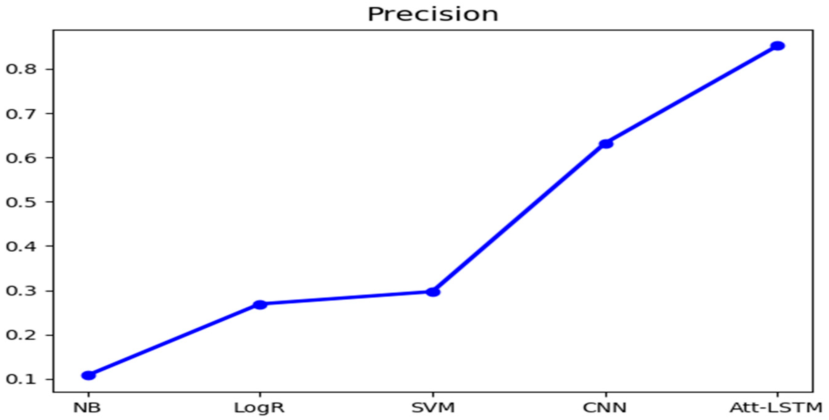
Precision: the precision metric measures the capabilities of the models in the positive prediction. As shown in
Figure 3, for the student comment dataset, deep learning approaches performed better than the traditional machine learning algorithm. Att-LSTM performed best, with its precision of up to 85.23%, while NB had 10.76%. The linear models, LogR, and SVM achieved similar scores in precision. Note that these models were trained by using the same feature selection method.
Recall: a common metric used in machine learning. As shown in
Figure 4, the three algorithms of Att-LSTM, LogR, and SVM performed better than NB and CNN. For NB that achieved the lowest score of recall. This metric score can be improved if the training dataset is used. The recall of the CNN had a better recall score. This improvement can further be made by data quality.
F1-score: the achieved metric F1-scores of the algorithms are shown in
Figure 5. CNN and Att-LSTM had higher scores than NB, LogR, and SVM. All the models were evaluated by a combination of the accuracy and recall of the metrics. The traditional machine learning algorithms had a similar performance, while neural networks had also close results.
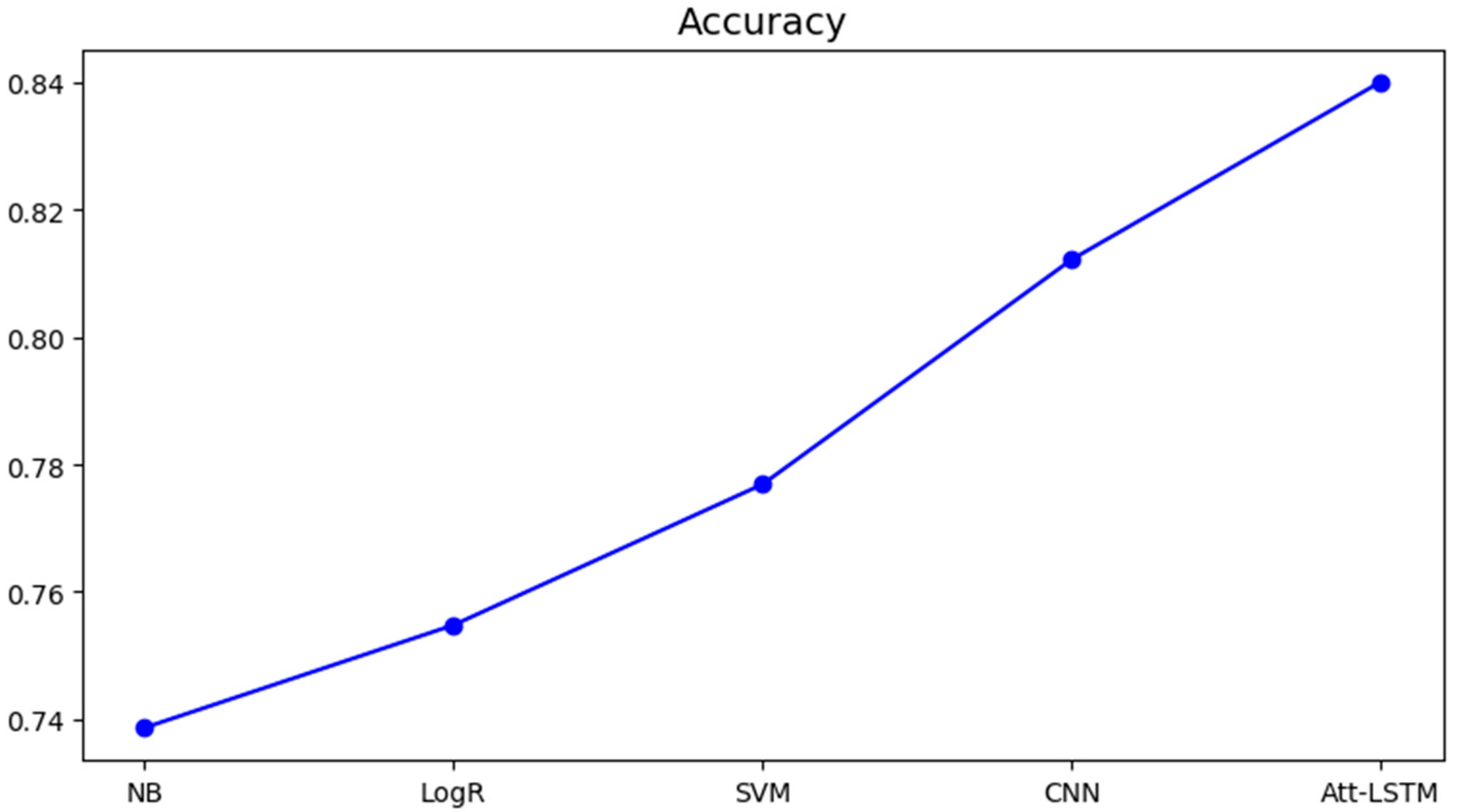
Accuracy:
Figure 6 shows the results of the metric of accuracy for the five algorithms. It evaluates the performance of the correct prediction on the student dataset. Att-LSTM and CNN produced higher accuracy than traditional approaches. Note that the accuracy was calculated by regarding the negative cases with one or more correct keywords and incorrect keywords as true.
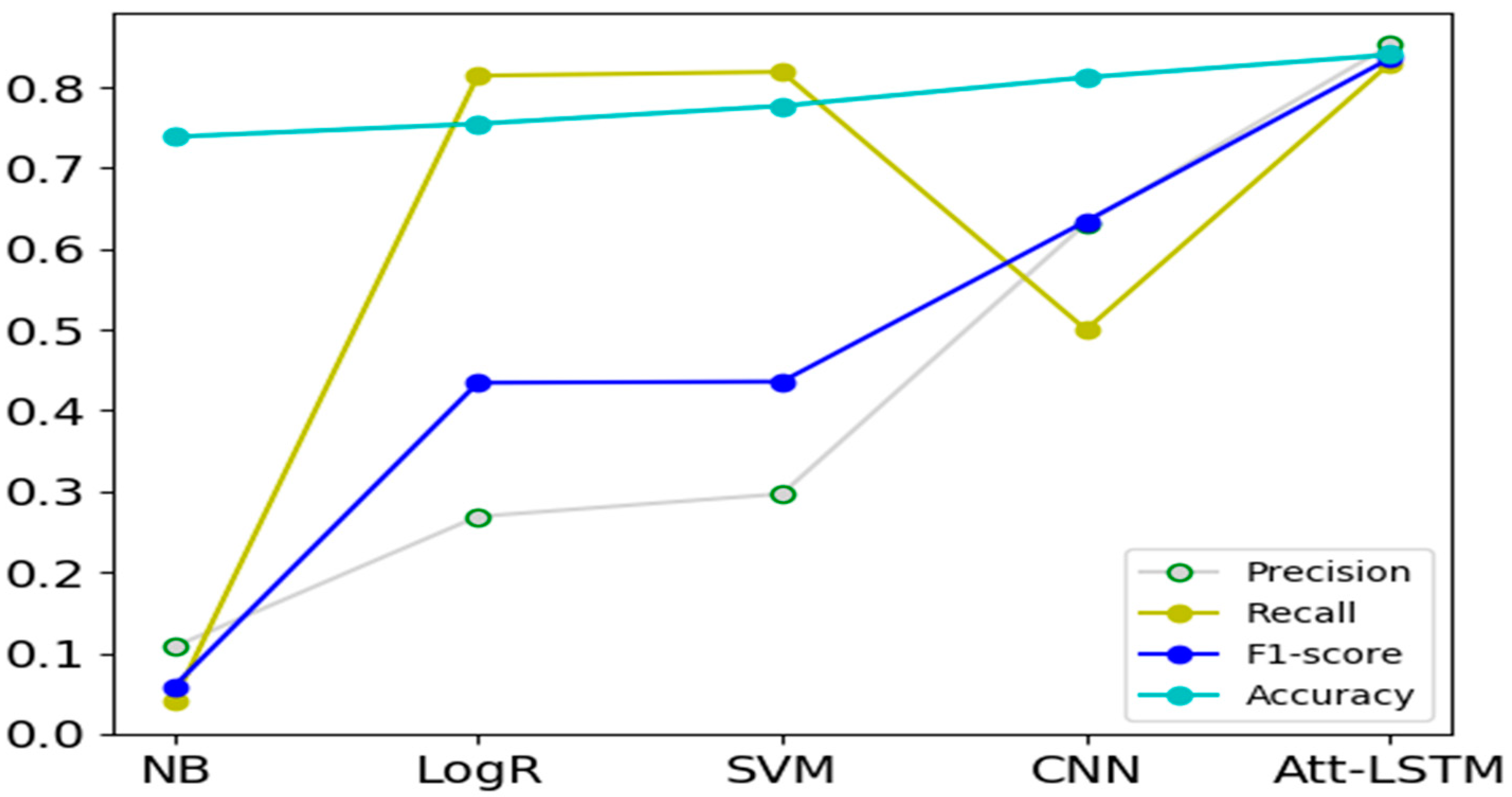
For predicting the topic keywords, we compared the five machine learning algorithms against the dataset of student comments in our experiments. Overall, neural networks performed better than traditional machine learning algorithms but took longer running times. In particular, Att-LSTM had achieved the highest performance in terms of the four metrics of precision, recall, F1 score, and accuracy, as shown in
Table 3 and
Figure 7. CNN performed a little bit lower than Att-LSTM, but higher than NB, LogR, and SVM. Taking less time on their training and predictions, NB, LogR, and SVM relied on the manually selected features for the training. Such features selection could affect their performance.
5. Visualization of Student Online Comments
So far, we have reported our comparisons of the five algorithms on extracting topic keywords from the student comments. However, the question of why these algorithms are working on this particular type of our dataset remains unanswered. Are there any patterns in student comments? If there are no regularities in these comments, the algorithms cannot detect or predict any categories. In this section, we make use of visual analysis [
67,
68,
69,
70,
71,
72,
73] to better understand student comments and to compare the degree of consistency and symmetry among the visualization results against some algorithm results. In particular, we first find some patterns in the student comments of the ITC-114 database and then visualize the keywords in these comments. From the experiments, it has been demonstrated that: (1) the visualization results provide some explanations of why the machine learning algorithms are capable of finding the categories; and (2) the resulting keywords produced by some algorithms are consistent with the visualization results.
5.1. Patterns in Student Comments
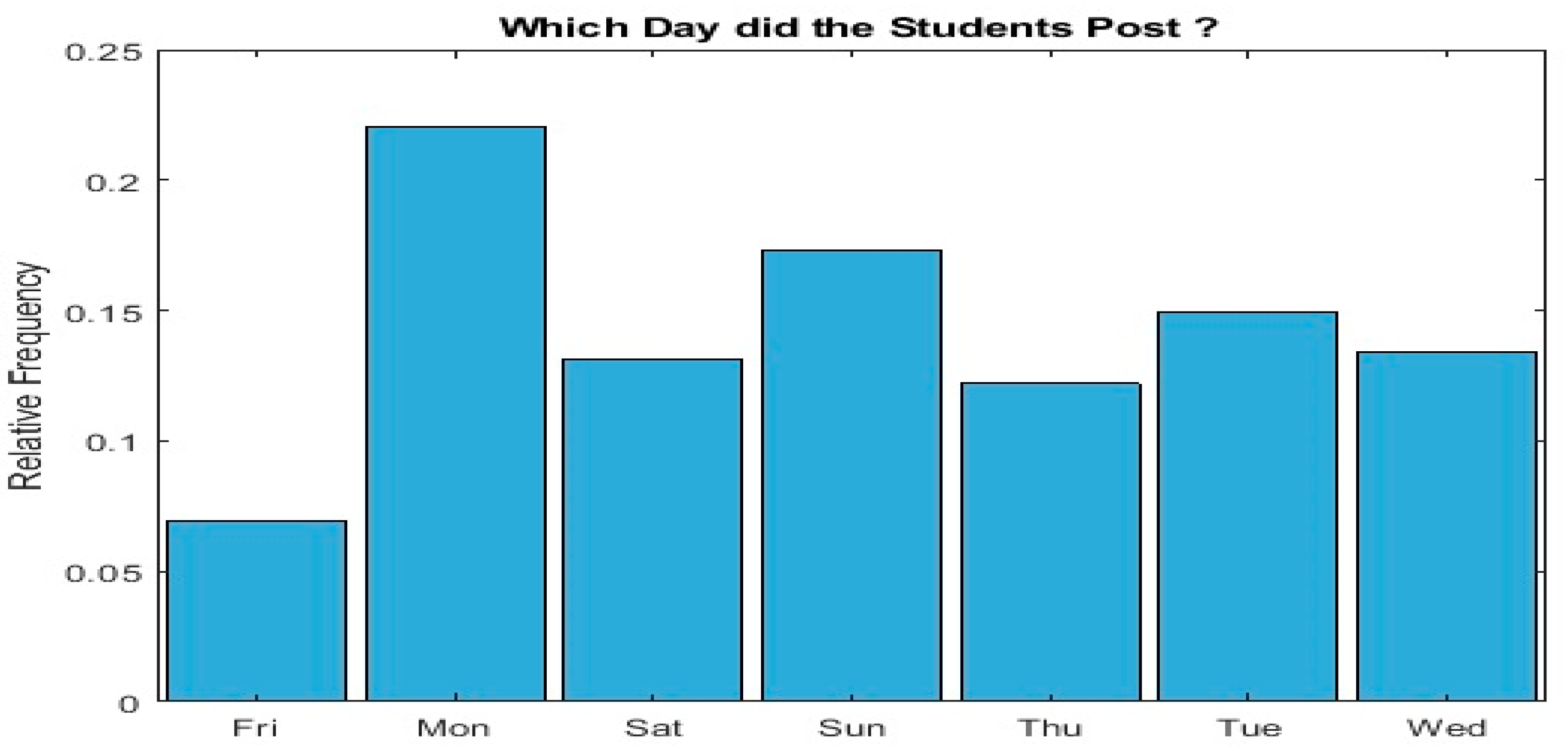
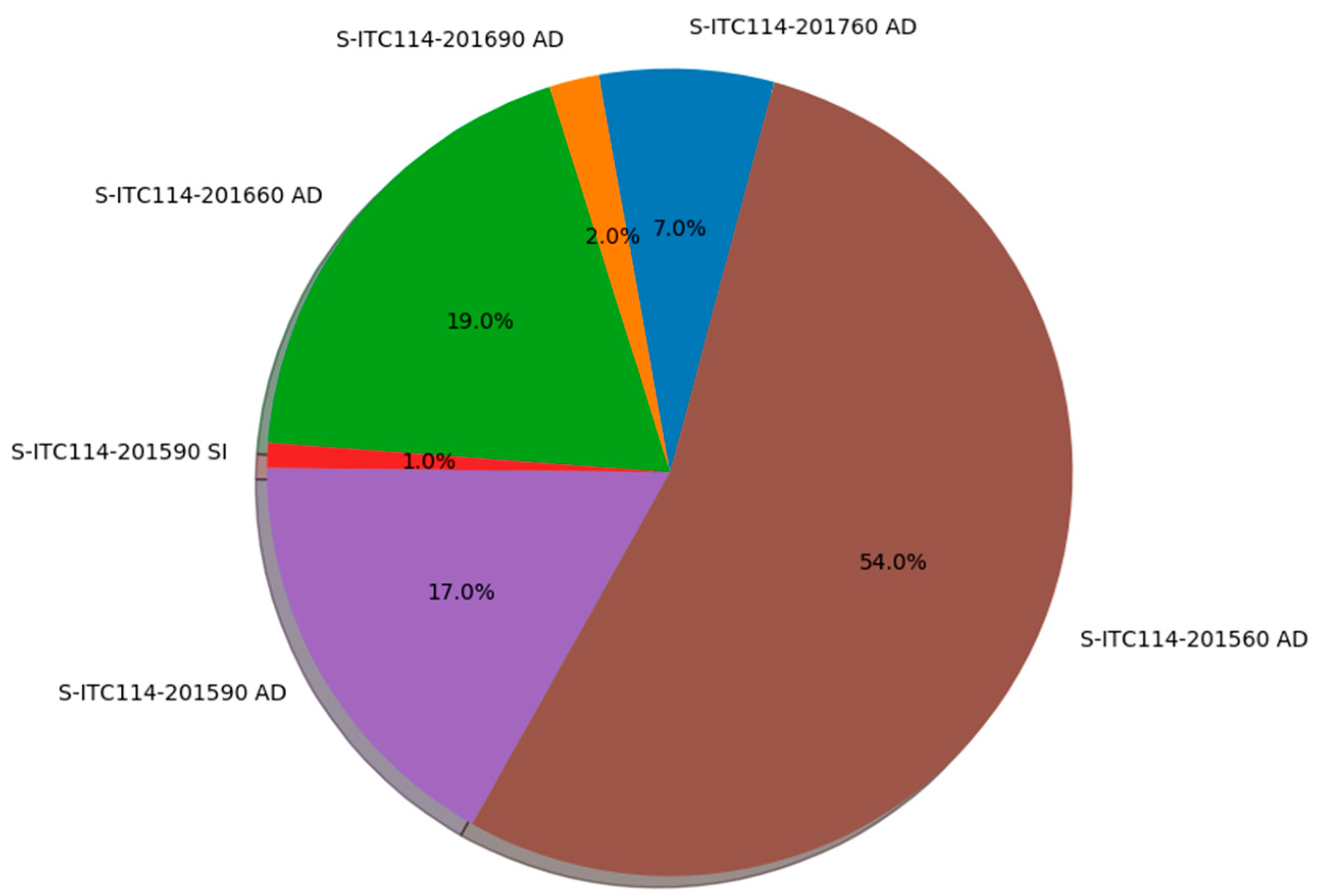
As shown in
Figure 8, we examine the number of comments on different days and over different teaching sessions of the ITC-114 database.
The percentages of comments from the ITC-114 database on different days are 22.05% for Monday, 17.32% for Sunday, 14.96% for Tuesday, 13.39% for Wednesday, 13.12% for Saturday, 12.20% for Tuesday, and 6.96% for Friday.
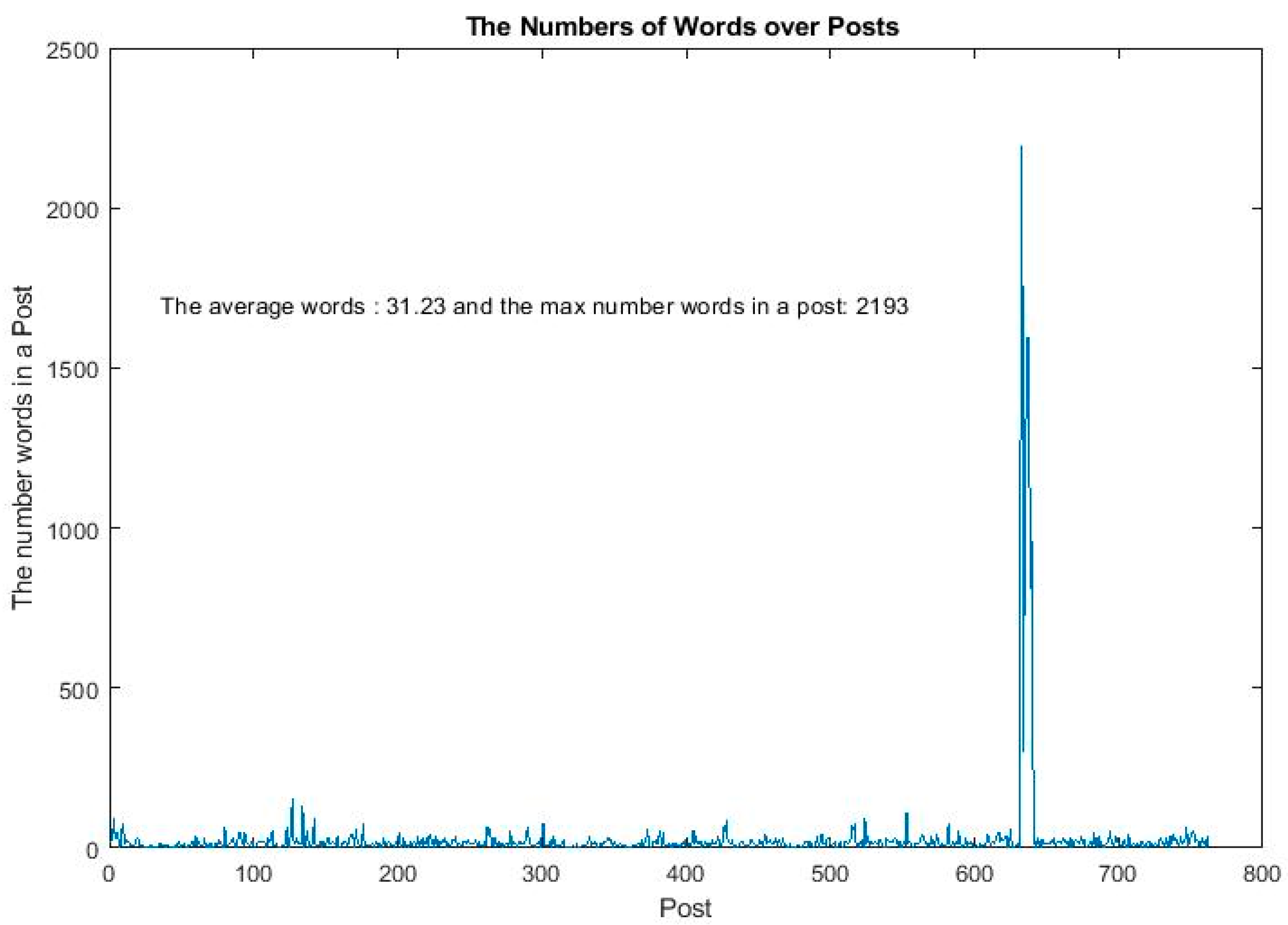
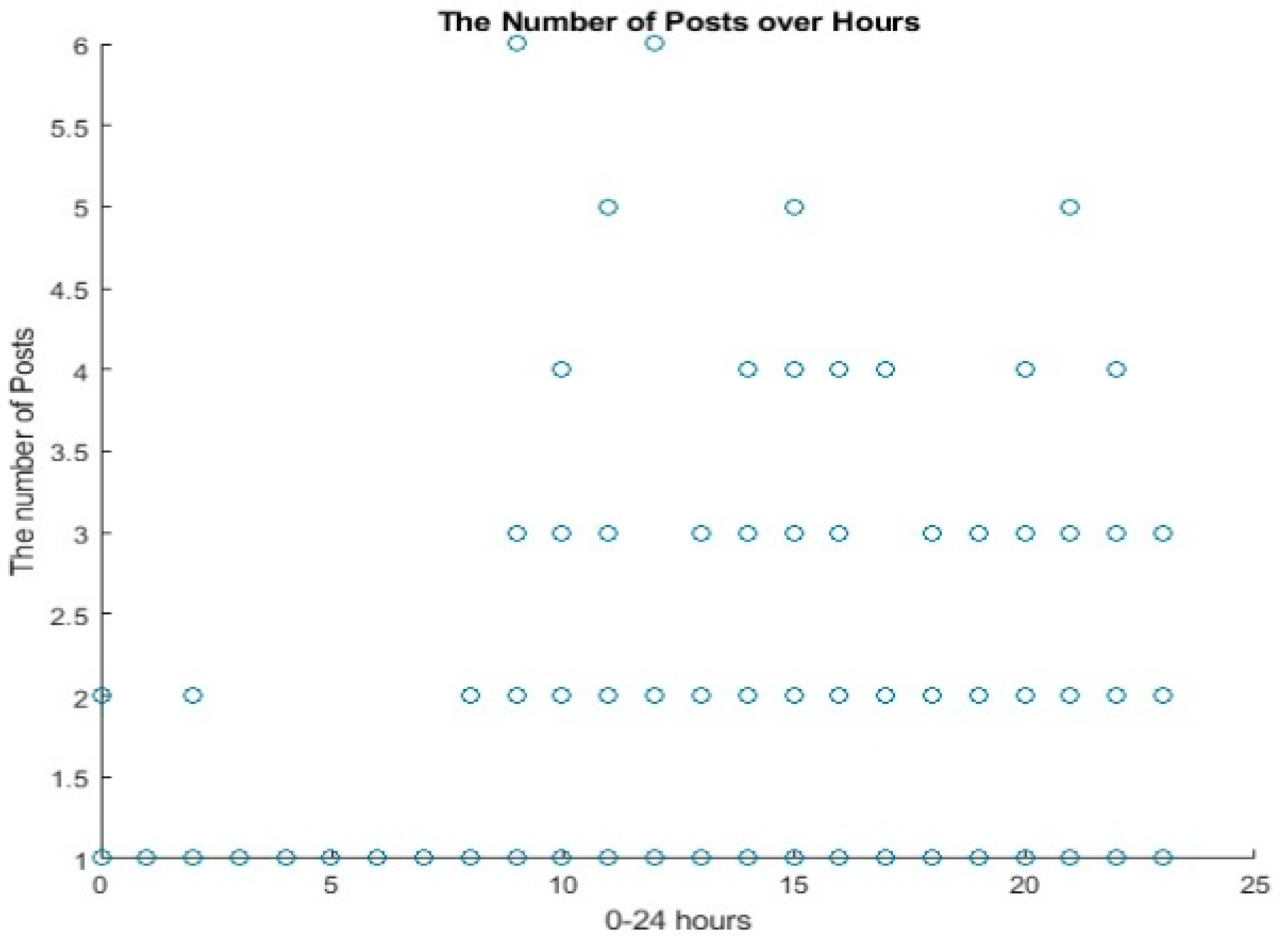
Next, the number of words in the posts and the number of words posted over hours from the ITC-114 database are shown in
Figure 9.
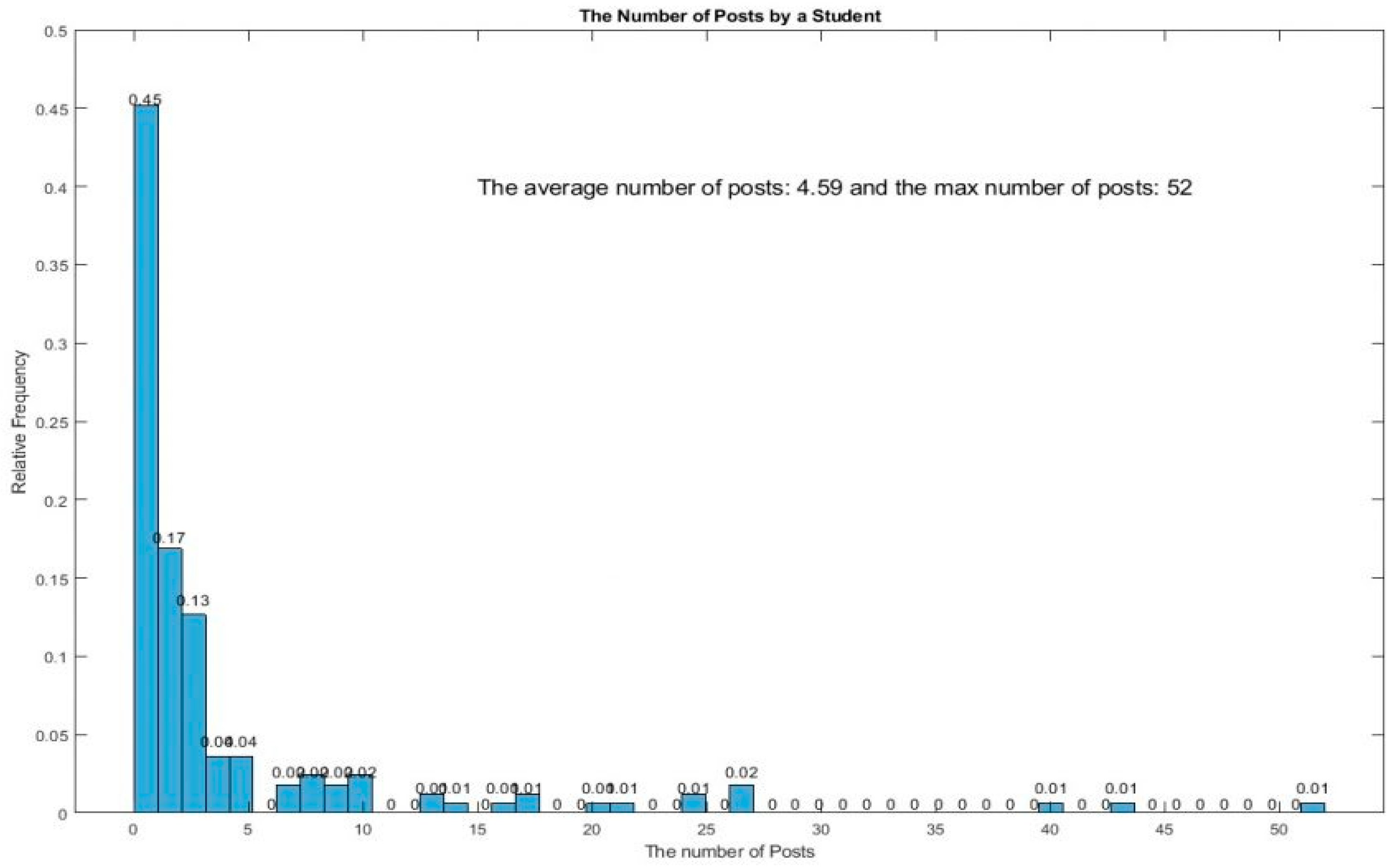
The distribution of comments by per student in the dataset of ITC-114 is shown in
Figure 10.
Visualization of the patterns in student comments aims to disclose the possible relationships between comments from the time perspective. We can regard the number of comments posted on different weekdays by different students or one student as time–serial data. In other words, these comments contain spatiotemporal information that may be captured by Att-LSTM. This is because the cells in LSTM can remember information over time intervals and use their gates to regulate the flow of information. However, we cannot see the obvious connections between the comments posted based on time and the results of Att-LSTM in our experiments. This may be because the dataset is not big enough or topics of comments do not have the spatiotemporal characteristics that are useful for Att-LSTM.
5.2. Keywords in Student Comments
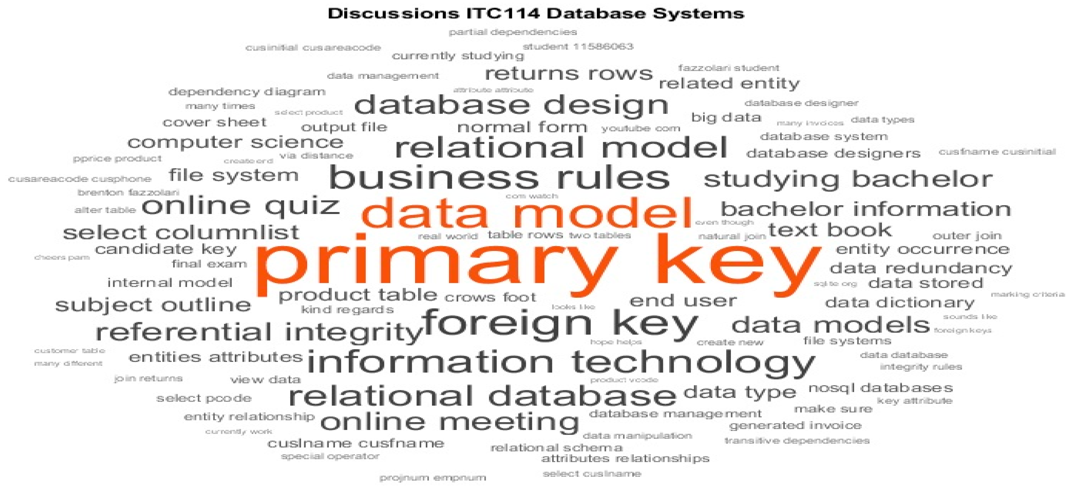
The word cloud of keyword frequencies in the comments is shown in
Figure 11.
This cloud is based on counting word pairs (bigrams) in comments. The more frequent the pairs, the bigger the sizes of their display in the cloud visualization are. The top 10 bigrams in our dataset are given as follows:
From
Table 4, we could see that the most important and difficult concepts related to the subject content have appeared in the student comments. We compare this visualization results with the keywords used in category results from the machine learning algorithms. We find that the word cloud is largely consistent with those by NB but little with Att-LSTM. For example, the category of the
concept identified by NB shares the highest number of the same keywords in the visualization. This may be because NB uses individual keywords as the feature for clustering labels without considering the semantic relationships between keywords. In this sense, it is similar to the word cloud that is based on the occurrence frequency of keywords in all the comments from a particular category.
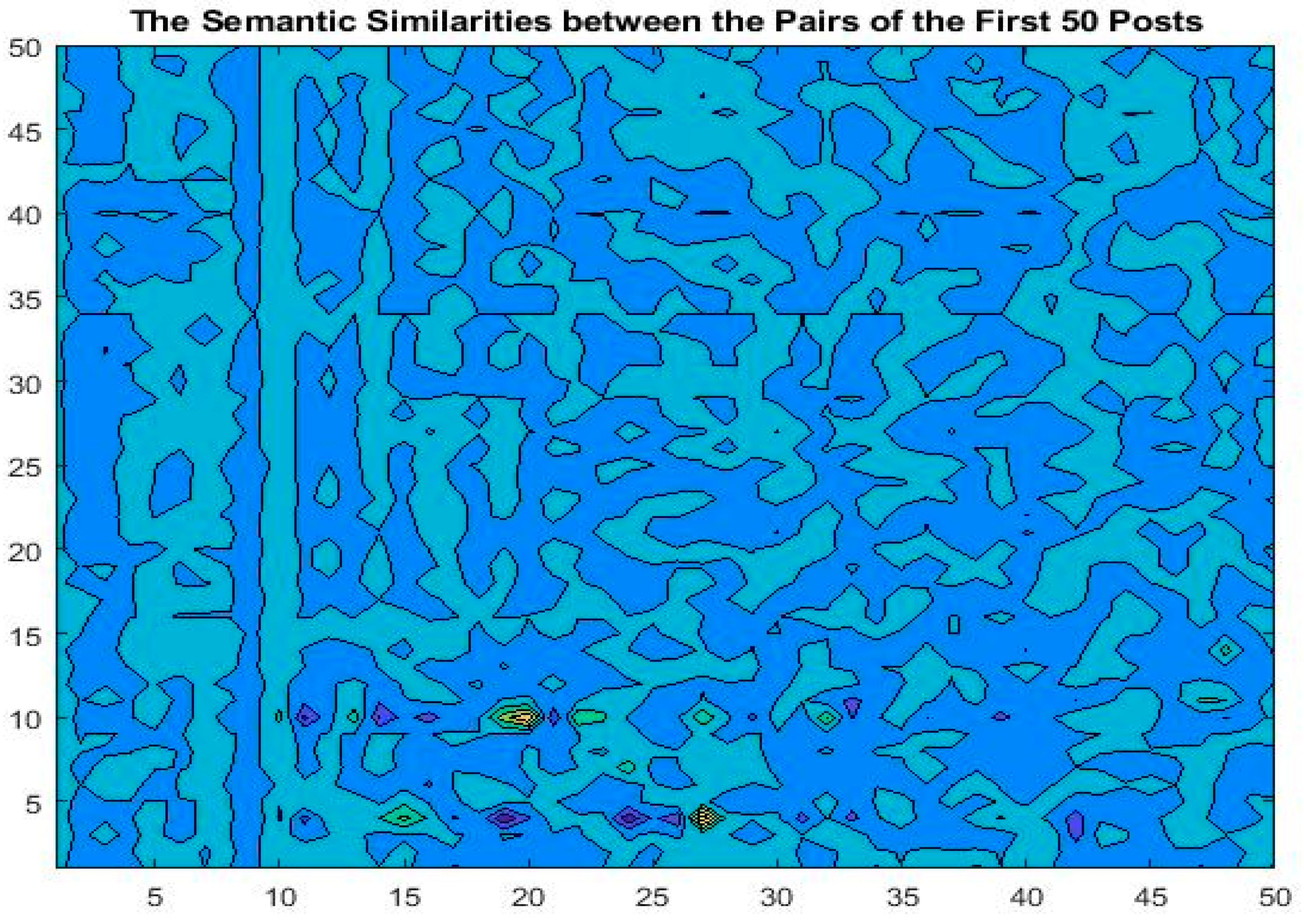
Finally, we visualize the semantic similarities between the pairs of the first 50 comments in ITC-114 in
Figure 12. For this, we first regard the first 50 comments as a collection and represent it as a matrix where each row is the TF–IDF scores of its keywords of a comment. Second, the similarity scores of all the comments (rows or columns) are calculated by using the pairwise cosine seminaries. As shown in
Figure 12, the visualization demonstrates that there are some degrees of similarities among the comments. This fact partially explains why learning algorithms can detect the categories of the comments. Further, we examine the similarity visualization of each category and the results by the compared algorithms. Some keywords in the clustered detected by Att-LSTM appear in the areas with relatively high similarity scores in the visualization. However, other algorithms produce the results that are marginally similar to the visual presentation.
After comparing what the algorithms produce, we conclude that results from some algorithms and visualization are consistent (and symmetry) to some extent. Further, we first divided a teaching session into several stages, such as introduction, assignment, online meeting, and exam. By companion, we then find that the extracted topics from the messages posted at the same stages were, almost, a reflection symmetry to those from different sessions. This is also reflected in
Figure 12 with some symmetry. This is because the data has not only the regularizes, but also some symmetry.
This work implies that we should consider actionable insight from the results of the algorithms and visualization. Actionable insight is the result of data-driven analytics of patterns that occur in student comments. By analyzing the comments—important data regarding online students—the lecturers can develop an understanding of students’ needs and expectations. More importantly, we can make data-informed decisions. On Mondays and Tuesdays, we may, for example, post our questions and read student comments on discussion boards, according to the identified categories by the algorithm. This comprehensive data analysis will shed light into optimal ways of creating meaningful learning experiences for students.
6. Conclusions
Online comments from students can provide an effective way of teaching and receiving feedback. How to automatically extract insightful information from these comments are important. In this work, we rely on machine learning algorithms to extract topic keywords from student comments to predict their topics. By doing so, we can summarize the information of online subject posts for improving the quality of learning and teaching in higher education.
In this paper, we presented the results of the compared performances of five algorithms given the same task of extracting topic keywords from student comment dataset. The selected methods ranged from traditional approaches to deep learning algorithms. They were compared against the same dataset and evaluated by the five metrics. From our experiments, our conclusions are as follows. The performance of the compared statistical algorithms, though being trained faster depends on the selected features. Deep learning algorithms achieved great accuracy, but with more training time. Of the two deep learning approaches compared, Att-LSTM performs the best in terms of all the metrics used. A combination method may perform better than any single approach due to overcoming limitations. Moreover, the quality of the dataset affected the results.
During the past decade, machine learning algorithms have demonstrated promising performances in a wide range of application areas. However, they are still limited in educational settings, particularly for higher education. In universities, many text tasks are usually time-consuming. Machine learning algorithms can automatically assist in completing these tasks, as demonstrated in this work.


