A Numerical Schemefor the Probability Density of the First Hitting Time for Some Random Processes


Abstract
1. Preliminaries
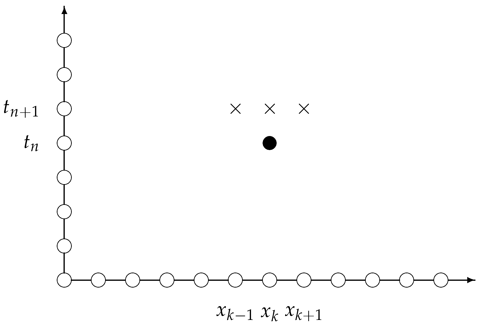
2. Discrete Model
- (a)
- it is strictly diagonally dominant,
- (b)
- its off-diagonal entries are less than or equal to zero, and
- (c)
- its diagonal entries are greater than zero.
- We use the notation to represent that all the components of are nonnegative.
- If the components of are less than or equal to 1, then we denote this by . Note that if and only if , where is the vector of the same dimension of whose components are equal to 1.
- If both and are satisfied, then we will write .
- We use the nomenclature to denote that . Obviously, this represents that each component of is less then or equal to the corresponding component of .
- Finally, we use to mean that , and are all satisfied.
- (a)
- , for each , and
- (b)
- and , for each .
- (a)
- , for each , and
- (b)
- and , for each .
3. Numerical Properties
4. Discussion and Conclusions
- Regarding the calculation of the first hitting time densities, only some few solutions are known in exact form for certain types of boundaries [4,5]. In every other case, numerical schemes should be considered and, in that sense, the present work contributes to the development of reliable numerical models to approximate the densities of first hitting times. However, we must point out that those densities can also be approximated by numerical schemes derived from the approximation to the associated integral equations. It is worth pointing out that some software has been developed following that approach [40]. The author of the present manuscript has followed a different approach, but the comparison between the present scheme and that reported in [40] is an interesting topic of investigation. However, extensive tests would need to be carried out under similar computational conditions. To start with, the codes must be in the same language and tests must be performed under the same computational architecture. To this day, the author has not devoted time to perform these tests, but it is an interesting task that the author of this work intends to carry out in the future.
- We must mention that it is possible to generalize the numerical procedure proposed in this work to account for more general stochastic processes than that considered herein, though some suitable adjustments are needed to that effect. As an example, it is well known that the probability distribution of the first passage time for Lévy time-charged Brownian motion with drift is a solution of a time-fractional advection–diffusion equation subjected to initial-boundary conditions [41]. In that case, the present approach can be modified to account for the presence of Caputo time-fractional derivatives and approximate the solutions of the associated partial differential equation. However, the structural and numerical analysis of that scheme would require a substantial amount of more effort and time. That could be the research topic of some independent report in the near future.
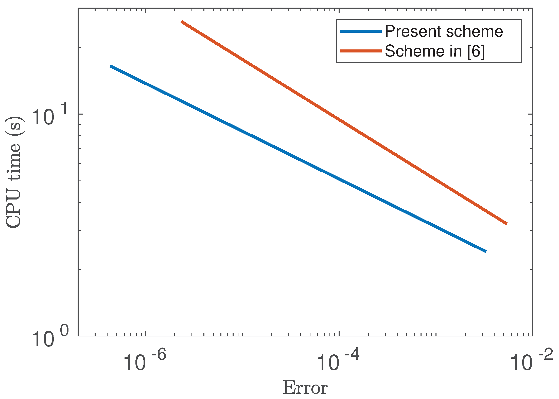
- It is important to point out that the same mathematical problem was considered in the work [6]. In that paper, the authors proposed a finite-difference scheme to approximate the probability distribution of the first hitting time associated with the same problem investigated in the present manuscript. The present approach has more advantages, though. To start with, the current numerical model is easier to implement computationally than that investigated in [6]. This fact can be easily checked from the Matlab code in Appendix A. Moreover, various theoretical and numerical advantages in the present approach are described below in the conclusions.
- The numerical scheme presented in this work may be relatively simple, but the analysis is rigorous and has various advantages. For example, it preserves the positivity, the boundedness and the monotonicity of the numerical solutions. This is an important feature in view that the relevant solutions of the parabolic problem considered herein possess these properties. The existence and uniqueness of solutions was thoroughly established here. Moreover, the scheme proposed in this work was theoretically analyzed for the numerical properties. Another advantage of our present approach is that the proofs of stability and convergence do not require additional conditions other than those asked to guarantee the existence of solutions.
- The numerical model introduced in the present work has a much easier computational implementation, in view that the system to solve at each time step is simpler. Indeed, the simplified Matlab program to obtain the simulations in this manuscript is that presented in Appendix A. Notice the simplicity of the code. Obviously, the computer program may be simplified or generalized even more.
- The current discretization presents spatial symmetry.
- The analysis of stability is the numerical model of the present manuscript was carried out without assuming that the matrices depend on the approximations at the time . This is a strong limitation of the results in [6]. Indeed, in that work, the authors needed to assume that the matrices did not depend on , which was an unrealistic assumption.
- The limitations of [6] described in the previous remark carried over to the analysis of convergence. Indeed, the model proposed in that paper had order of convergence , but the hypotheses to guarantee that order were utterly restrictive and unrealistic.
- Stability and convergence were established in the present discretization. On the contrary, the paper mentioned above requires additional constraints which limit the approach severely. Our present approach has convergence order , but the theoretical result need less constraints to guarantee this order. We have performed numerical tests of convergence (not presented here in order to avoid redundancy), and they show that the present scheme has linear order of convergence in the temporal variable, and second order in the spatial domain.
- It is worth mentioning that there are various reports available in the literature in which problems with moving boundaries have been investigated numerically [42,43,44,45,46,47,48]. However, the present is an easy-to-implement model which preserves various advantages from the structural and numerical points of view.
Funding
Acknowledgments
Conflicts of Interest
Appendix A. Matlab Code

References
- Strassen, V. Almost sure behaviour of sums of independent random variables and martingales. In Proceedings of the Fifth Berkeley Symposium; University of California Press: Berkeley, CA, USA, 1967; Volume 2, pp. 315–343. [Google Scholar]
- Ferebee, B. The tangent approximation to one-sided Brownian exit densities. Z. Wahrscheinlichkeitstheorie Verwandte Geb. 1982, 61, 309–326. [Google Scholar] [CrossRef]
- Palyulin, V.V.; Blackburn, G.; Lomholt, M.A.; Watkins, N.W.; Metzler, R.; Klages, R.; Chechkin, A.V. First passage and first hitting times of Lévy flights and Lévy walks. New J. Phys. 2019, 21, 103028. [Google Scholar] [CrossRef]
- Giorno, V.; Nobile, A.; Ricciardi, L.; Sato, S. On the evaluation of first-passage-time probability densities via non-singular integral equations. Adv. Appl. Probab. 1989, 21, 20–36. [Google Scholar] [CrossRef]
- Gutiérrez-Jáimez, R.; Román-Román, P.; Torres-Ruiz, F. A note on the Volterra integral equation for the first-passage-time density. J. Appl. Probab. 1995, 32, 635–648. [Google Scholar]
- Macías-Díaz, J.E.; Villa-Morales, J. A structure-preserving method for the distribution of the first hitting time to a moving boundary for some Gaussian processes. Comput. Math. Appl. 2017, 74, 1799–1812. [Google Scholar] [CrossRef]
- Salminen, P. On the first hitting time and the last exit time for a Brownian motion to/from a moving boundary. Adv. Appl. Probab. 1988, 20, 411–426. [Google Scholar] [CrossRef]
- Lipton, A.; Kaushansky, V. On the first hitting time density for a reducible diffusion process. Quant. Financ. 2020, 20, 723–743. [Google Scholar] [CrossRef]
- Abundo, M. On the first hitting time of a one-dimensional diffusion and a compound Poisson process. Methodol. Comput. Appl. Probab. 2010, 12, 473–490. [Google Scholar] [CrossRef]
- Ettl, W. Markov Processes Between Moving Barriers—Moments of the First Hitting Time of Retaining or Absorbing Barrier. In Insurance and Risk Theory; Springer: Berlin/Heidelberg, Germany, 1986; pp. 239–245. [Google Scholar]
- Lo, C.F.; Hui, C.H. Computing the first passage time density of a time-dependent Ornstein—Uhlenbeck process to a moving boundary. Appl. Math. Lett. 2006, 19, 1399–1405. [Google Scholar] [CrossRef]
- Aurzada, F.; Kramm, T. The first passage time problem over a moving boundary for asymptotically stable Lévy processes. J. Theor. Probab. 2016, 29, 737–760. [Google Scholar] [CrossRef][Green Version]
- Zhang, S.; Geng, J. Efficiently pricing continuously monitored barrier options under stochastic volatility model with jumps. Int. J. Comput. Math. 2017, 94, 2166–2177. [Google Scholar] [CrossRef]
- Nishioka, K. The first hitting time and place of a half-line by a biharmonic pseudo process. Jpn. J. Math. New Ser. 1997, 23, 235–280. [Google Scholar] [CrossRef][Green Version]
- Liu, W. Analytical study on a moving boundary problem of semispherical centripetal seepage flow of Bingham fluid with threshold pressure gradient. Int. J. Non-Linear Mech. 2019, 113, 17–30. [Google Scholar] [CrossRef]
- Čanić, S.; Mikelić, A.; Kim, T.B.; Guidoboni, G. Existence of a unique solution to a nonlinear moving-boundary problem of mixed type arising in modeling blood flow. In Nonlinear Conservation Laws and Applications; Springer: Berlin/Heidelberg, Germany, 2011; pp. 235–256. [Google Scholar]
- Crank, J.; Gupta, R.S. A moving boundary problem arising from the diffusion of oxygen in absorbing tissue. IMA J. Appl. Math. 1972, 10, 19–33. [Google Scholar] [CrossRef]
- Sassa, S.; Sekiguchi, H.; Miyamoto, J. Analysis of progressive liquefaction as a moving-boundary problem. Geotechnique 2001, 51, 847–857. [Google Scholar] [CrossRef]
- Purlis, E.; Salvadori, V.O. Bread baking as a moving boundary problem. Part 1: Mathematical modelling. J. Food Eng. 2009, 91, 428–433. [Google Scholar] [CrossRef]
- Cui, S.; Escher, J. Asymptotic behaviour of solutions of a multidimensional moving boundary problem modeling tumor growth. Commun. Partial Differ. Eqs. 2008, 33, 636–655. [Google Scholar] [CrossRef]
- Benard, C.; Gobin, D.; Zanoli, A. Moving boundary problem: Heat conduction in the solid phase of a phase-change material during melting driven by natural convection in the liquid. Int. J. Heat Mass Transf. 1986, 29, 1669–1681. [Google Scholar] [CrossRef]
- Muntean, A.; Böhm, M. A moving-boundary problem for concrete carbonation: Global existence and uniqueness of weak solutions. J. Math. Anal. Appl. 2009, 350, 234–251. [Google Scholar] [CrossRef]
- Liu, W.; Yao, J.; Chen, Z.; Zhu, W. An exact analytical solution of moving boundary problem of radial fluid flow in an infinite low-permeability reservoir with threshold pressure gradient. J. Pet. Sci. Eng. 2019, 175, 9–21. [Google Scholar] [CrossRef]
- Kumar, A.; Rajeev. A moving boundary problem with space-fractional diffusion logistic population model and density-dependent dispersal rate. Appl. Math. Model. 2020, 88, 951–965. [Google Scholar] [CrossRef]
- Garshasbi, M.; Malek Bagomghaleh, S. An iterative approach to solve a nonlinear moving boundary problem describing the solvent diffusion within glassy polymers. Math. Methods Appl. Sci. 2020, 43, 3754–3772. [Google Scholar] [CrossRef]
- Egorova, V.N.; Tan, S.H.; Lai, C.H.; Company, R.; Jódar, L. Moving boundary transformation for American call options with transaction cost: Finite difference methods and computing. Int. J. Comput. Math. 2017, 94, 345–362. [Google Scholar] [CrossRef]
- Bakhta, A.; Ehrlacher, V. Cross-diffusion systems with non-zero flux and moving boundary conditions. ESAIM Math. Model. Numer. Anal. 2018, 52, 1385–1415. [Google Scholar] [CrossRef]
- Sakakibara, K.; Miyatake, Y. A fully discrete curve-shortening polygonal evolution law for moving boundary problems. arXiv 2020, arXiv:1912.00545. [Google Scholar] [CrossRef]
- Wang, L.; Wang, Y. Multisymplectic structure-preserving scheme for the coupled Gross—Pitaevskii equations. Int. J. Comput. Math. 2020, 1–24. [Google Scholar] [CrossRef]
- Chen, H.; Lv, W. Kronecker product-based structure preserving preconditioner for three-dimensional space-fractional diffusion equations. Int. J. Comput. Math. 2020, 97, 585–601. [Google Scholar] [CrossRef]
- Macías-Díaz, J.E.; Puri, A. An explicit positivity-preserving finite-difference scheme for the classical Fisher–Kolmogorov–Petrovsky–Piscounov equation. Appl. Math. Comput. 2012, 218, 5829–5837. [Google Scholar] [CrossRef]
- Macías-Díaz, J.E.; Szafrańska, A. Existence and uniqueness of monotone and bounded solutions for a finite-difference discretization à la Mickens of the generalized Burgers–Huxley equation. J. Differ. Eqs. Appl. 2014, 20, 989–1004. [Google Scholar] [CrossRef]
- Zhang, X.; Shu, C.W. On positivity-preserving high order discontinuous Galerkin schemes for compressible Euler equations on rectangular meshes. J. Comput. Phys. 2010, 229, 8918–8934. [Google Scholar] [CrossRef]
- Yu, Y.; Deng, W.; Wu, Y. Positivity and boundedness preserving schemes for space–time fractional predator–prey reaction–diffusion model. Comput. Math. Appl. 2015, 69, 743–759. [Google Scholar] [CrossRef]
- Macías-Díaz, J.E.; Hendy, A.S.; De Staelen, R.H. A compact fourth-order in space energy-preserving method for Riesz space-fractional nonlinear wave equations. Appl. Math. Comput. 2018, 325, 1–14. [Google Scholar] [CrossRef]
- Macías-Díaz, J.E.; Puri, A. On the transmission of binary bits in discrete Josephson-junction arrays. Phys. Lett. A 2008, 372, 5004–5010. [Google Scholar] [CrossRef]
- Fujimoto, T.; Ranade, R.R. Two characterizations of inverse-positive matrices: The Hawkins-Simon condition and the Le Chatelier-Braun principle. Electron. J. Linear Algebra 2004, 11, 6. [Google Scholar] [CrossRef][Green Version]
- Chen, S.; Liu, F.; Turner, I.; Anh, V. An implicit numerical method for the two-dimensional fractional percolation equation. Appl. Math. Comput. 2013, 219, 4322–4331. [Google Scholar] [CrossRef]
- Tian, G.X.; Huang, T.Z. Inequalities for the minimum eigenvalue of M-matrices. ELA Electron. J. Linear Algebra 2010, 20, 291–302. [Google Scholar] [CrossRef]
- Román-Román, P.; Serrano-Pérez, J.; Torres-Ruiz, F. An R package for an efficient approximation of first-passage-time densities for diffusion processes based on the FPTL function. Appl. Math. Comput. 2012, 218, 8408–8428. [Google Scholar] [CrossRef]
- Abundo, M.; Ascione, G.; Carfora, M.; Pirozzi, E. A fractional PDE for first passage time of time-changed Brownian motion and its numerical solution. Appl. Numer. Math. 2020, 155, 103–118. [Google Scholar] [CrossRef]
- Bretti, G.; Natalini, R.; Piccoli, B. A fluid-dynamic traffic model on road networks. Arch. Comput. Methods Eng. 2007, 14, 139–172. [Google Scholar] [CrossRef]
- Bretti, G.; Piccoli, B. A tracking algorithm for car paths on road networks. SIAM J. Appl. Dyn. Syst. 2008, 7, 510–531. [Google Scholar] [CrossRef][Green Version]
- Cutolo, A.; Piccoli, B.; Rarità, L. An upwind-Euler scheme for an ODE-PDE model of supply chains. SIAM J. Sci. Comput. 2011, 33, 1669–1688. [Google Scholar] [CrossRef][Green Version]
- Pasquino, N.; Rarità, L. Automotive processes simulated by an ODE-PDE model. In Proceedings of the EMSS 2012, Vienna, Austria, 19–21 September 2012; pp. 352–361. [Google Scholar]
- de Falco, M.; Gaeta, M.; Loia, V.; Rarità, L.; Tomasiello, S. Differential quadrature-based numerical solutions of a fluid dynamic model for supply chains. Commun. Math. Sci. 2016, 14, 1467–1476. [Google Scholar] [CrossRef]
- Lattanzio, C.; Maurizi, A.; Piccoli, B. Modeling and simulation of vehicular traffic flow with moving bottlenecks. Proc. MASCOT09 2010, 15, 181–190. [Google Scholar]
- Lattanzio, C.; Maurizi, A.; Piccoli, B. Moving bottlenecks in car traffic flow: A PDE-ODE coupled model. SIAM J. Math. Anal. 2011, 43, 50–67. [Google Scholar] [CrossRef]


Publisher’s Note: MDPI stays neutral with regard to jurisdictional claims in published maps and institutional affiliations. |
© 2020 by the author. Licensee MDPI, Basel, Switzerland. This article is an open access article distributed under the terms and conditions of the Creative Commons Attribution (CC BY) license (http://creativecommons.org/licenses/by/4.0/).
Share and Cite
Macías-Díaz, J.E. A Numerical Schemefor the Probability Density of the First Hitting Time for Some Random Processes. Symmetry 2020, 12, 1907. https://doi.org/10.3390/sym12111907
Macías-Díaz JE. A Numerical Schemefor the Probability Density of the First Hitting Time for Some Random Processes. Symmetry. 2020; 12(11):1907. https://doi.org/10.3390/sym12111907
Chicago/Turabian StyleMacías-Díaz, Jorge E. 2020. "A Numerical Schemefor the Probability Density of the First Hitting Time for Some Random Processes" Symmetry 12, no. 11: 1907. https://doi.org/10.3390/sym12111907
APA StyleMacías-Díaz, J. E. (2020). A Numerical Schemefor the Probability Density of the First Hitting Time for Some Random Processes. Symmetry, 12(11), 1907. https://doi.org/10.3390/sym12111907