1. Introduction
The idea of overcoming the limitations of fluids’ thermal properties in the case of heat transfer processes was and still is very tempting. The concept of adding small solid particles to the fluids, characterized by much higher values regarding thermal properties (e.g., thermal conductivity), was already realized and resulted in the appearance of nanofluids. The Maxwell model [
1] predicts that an increasing volume fraction of particles leads to an increased value of thermal conductivity. Since the appearance of this model, a lot of effort was made to demonstrate the superior properties of the nanofluids over commonly used fluids [
2,
3,
4]. However, there is still an unequivocal conclusion on the positive effect of nanoparticle additions [
5,
6,
7]. Nevertheless, nanofluids are considered as a very promising medium for engineering applications and the addition of nanoparticles is treated as a passive method of heat transfer enhancement. Due to the very fast technology development, there is increasing demand for the transfer of high heat fluxes, therefore any idea to increase their transfer is welcomed. Simultaneous use of various methods of heat transfer enhancement is a natural response to this demand and resulted in a proposal of utilization of magnetic field together with nanofluids. Such a combination was a consequence of previous research on the strong magnetic field ability to control heat transfer processes for single-phase paramagnetic fluids. Published results [
8,
9,
10] confirmed this ability.
Investigation of nanofluid heat transfer influenced by a strong magnetic field is mostly performed by numerical methods. This approach has many advantages, such as availability of detailed information on the velocity and temperature fields or other parameters characterizing thermal and hydrodynamic flow aspects. The nanofluids in these investigations are commonly treated as single-phase fluids while their properties are modelled as weighted averages. These assumptions significantly simplify the calculations. It is also worth mentioning that mainly two-dimensional geometry is considered. The numerical analyses involves, for example, Lattice Boltzmann Methods (LBMs) [
11,
12,
13,
14], Finite-difference Method (FDM) [
15], Finite Element Method (FEM) [
16], Finite Volume Method (FVM) [
17], and Control Volume Finite Element Method (CVFEM) [
18]. Results coming from all investigations could be shortly concluded as heat transfer processes are augmented by increasing nanoparticle volume fractions and they are also attenuated under a magnetic field effect.
Coming to the nanofluid flow structure influenced by the magnetic environment, it could be said that there is no general tendency. Mixed convection of various nanofluids (consisting of water as a base fluid and Ag, Cu, CuO, Al
2O
3 and TiO
2 as solid particles) influenced by a magnetic field was discussed in [
19]. One of the observations coming from this report was that flow with one dominating cell could be changed by increasing the strength of the magnetic field to symmetrical three rolls flow, one above the other. Examination of aluminum oxide–water nanofluid free convection within cubic porous cavity was conducted in [
20]. Magnetic force was responsible for decreasing velocity component values (presented by
x and
z components); however, it did not change the symmetrical distribution of those parameters for Al
2O
3 nanoparticle concentration. The effect of silver nanoparticles’ volume fraction and magnetic field on convective heat transfer processes in cylindrical annulus enclosure was studied in [
21]. The velocity components’ values increased as a function of increasing nanoparticle concentrations. On the other hand, the pattern of isotherms was affected strongly and convection was suppressed by increasing the magnetic field. Investigations on the influence of magnetic and thermal gradients’ mutual orientations (at a different angle) on ferrofluid flow was studied in [
22]. Unicellular flow, rotating counter-clockwise, changed to the two-cell mode. Then, a single clockwise cell appeared for a varied angle, which showed that in such a case, the resultant force is strong enough to reverse the fluid flow. The phenomena of reverse flow was occurring when the thermo-magnetic convection force was dominant over the thermo-gravity convection—force names are as in the referenced article.
Since the experimental analysis presented in [
23] exhibited a different tendency than reported in the literature, referring to the influence of increasing nanoparticle concentration and magnetic field on the heat transfer processes, a numerical analysis of these issues was conducted. Moreover, the flow structure was considered as unknown, because of the opaqueness of the nanofluid. Therefore, the aim of this paper is to investigate a strong magnetic field’s ability to change diamagnetic nanofluid thermal convection inside differentially heated cubical enclosures placed in a Rayleigh–Benard configuration. To achieve the goal, the numerical approach of two-phase flow, namely the Euler–Euler approach, was utilized. The various Ag nanoparticle concentrations and magnetic induction values were considered at constant temperature differences. The focus was on the heat transfer processes, occurring in the enclosure and the flow structure without and with influence of a magnetic field. The Fast Fourier Transform (FFT) analysis was also conducted to deepen the understanding of occurring phenomena.
2. Considered System
The thermal convection of silver nanofluid in the Rayleigh–Benard configuration was subjected to a strong magnetic field. The silver nanofluid consisted of water as the base fluid and spherical silver nanoparticles of about 50 nm in diameter. Various concentrations of silver nanoparticles (0, 0.1, 0.25 and 0.5 vol.%) and various values of magnetic induction (in range 0–9 T) were analyzed. There are some publications referring to the properties of silver nanofluids [
24,
25], however, analyzed nanoparticle concentrations were different than presented in these publications. Therefore, in a small part of the numerical analysis, the nanofluid properties were determined in the basis of theoretical equations described in
Section 3.
The studied system was a cubical enclosure 0.032 m in size. The bottom horizontal wall was kept at a constant temperature equal to 299 K, while the top horizontal wall was at a constant temperature equal to 291 K. Remaining walls were considered adiabatic.
The enclosure was located in the magnetic field and distribution was calculated on the basis of characteristics of a real superconducting magnet (Superconducting Helium Free Magnet HF10-100VHT-B, SHI Cryogenics Europe GmbH, Darmstadt, Germany).
Magnetic Field
The stationary magnetic field was considered. The following set of equations (coming from the Maxwell equations) were utilized for calculations:
where:
H is a vector of the magnetic field strength [A/m],
B is a vector of the magnetic induction [T],
J is a vector of electric current density, which is a source of the magnetic field [A/m
2],
A is a vector of magnetic field potential [Wb/m] and
μ is the medium magnetic permeability [H/m], resulting in the final equation:
which should be solved for the analyzed system regarding variable
A, when the electrical current density is known. The boundary conditions of the magnetic field potential equal to zero was set at the large shell (4 m diameter) covering the electrical solenoid. Calculations were conducted in Comsol software.
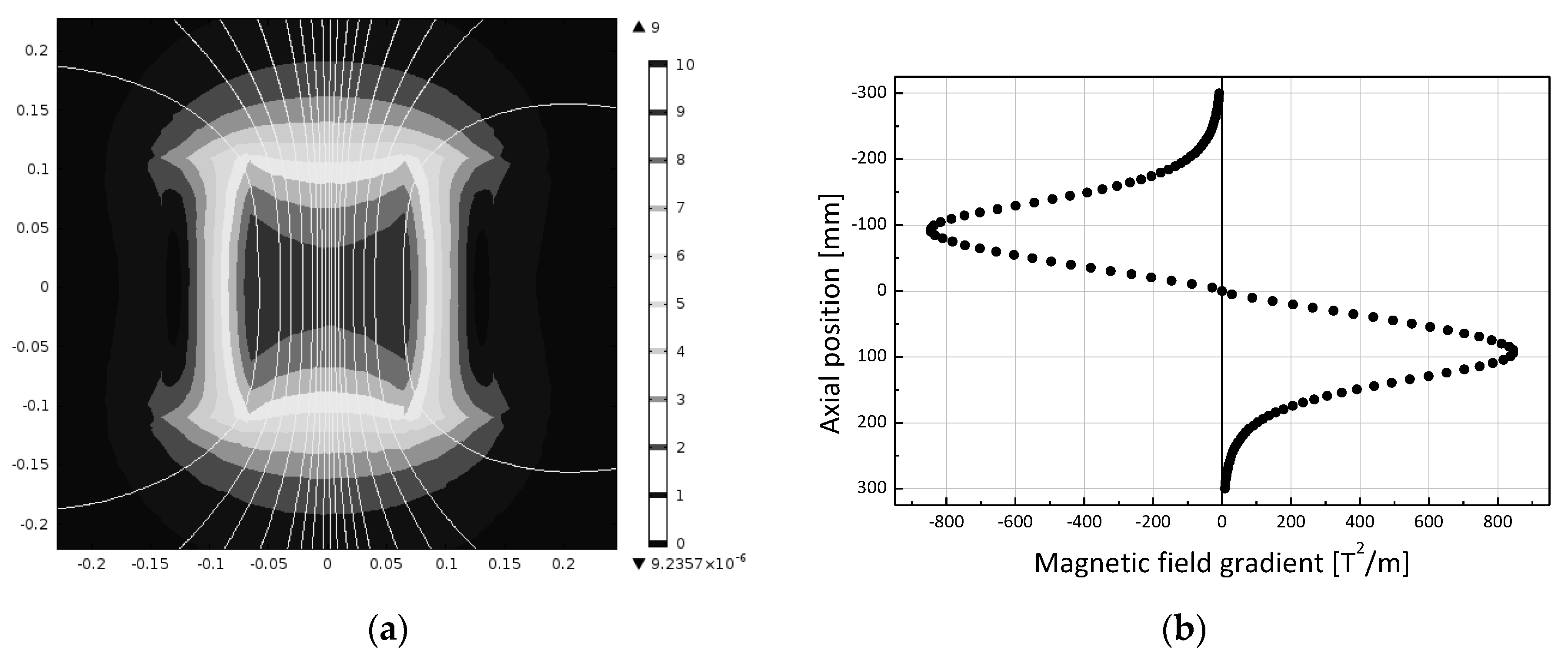
The magnetic induction distribution in the vicinity of the electrical solenoid is shown in
Figure 1a, while the gradient of magnetic induction square is shown in
Figure 1b. The distribution of the magnetic induction square exhibit two maxima which are related to the strongest influence of magnetic buoyancy force. In the presented study, the enclosure was placed in the lower maximum.
3. Mathematical Modelling of Nanofluid Flow
As already mentioned, in the majority of published papers the nanofluid was treated as single-phase, characterized by the weighted average properties which are the functions of nanoparticle concentrations. In the presented research, the nanofluid was considered as a two-phase one. The properties of each component are presented in
Table 1.
The nanofluid was then treated as a mixture of two interpenetrating phases: the continuous water phase and the dispersed phase formed by the nanoparticles. Each phase is a separate one, therefore such an approach belongs to a class of separated flow (SF) models. The computational methods currently utilized for an analysis of two-phase SF flow can be classified into three categories [
26]: Euler–Euler (E-E), Euler–Lagrange (E-L) and Lagrange–Lagrange (L-L).
In the E-E model, each phase is treated as the continuous one, which is why the instantaneous continuum transport equations are used to describe it. In the E-L method, the so called “carrier” fluid phase dynamics is described in Eulerian frame of reference based on a continuum model, and the dispersed phase is described by a set of classical Newtonian rigid body dynamics equations in the Lagrange frame of reference. In the third category, L-L models, both phases are described in the Lagrangian frame of reference.
In the presented work, the E-E model was utilized. It should be added that the momentum exchange between the phases was taken as a one-way coupling condition. It occurs at the phase boundary due to friction introduced by the non-zero slip velocity and molecular viscosity of the carrier phase. The instantaneous equations, describing each of the phases, are represented by the balance of mass and momentum.
The mass balance, represented by the continuity equation, takes a particular form for each phase:
dispersed phase:
where:
ϕ is the volume fraction of the dispersed phase [-];
u,
v are the velocity vectors of the carrier and dispersed phases, respectively [m/s];
are the density of the carrier and dispersed phases, respectively, [kg/m
3].
The momentum balance equations for particular phases are as follows:
dispersed phase:
where
are the viscous stress tensors of the carrier and dispersed phases, respectively [N/m
2];
Fc and
Fd are the sum of body forces acting on the carrier phase and dispersed phase, respectively. Definitions of these forces are written as:
where
Fg and
Fm are the vectors of volumetric forces (gravitational and magnetic, [N/m
3]):
where:
g is the gravitational acceleration, [m/s
2];
ρ is the density, [kg/m
3];
β is the thermal expansion coefficient, [1/K];
T is the temperature, [K];
T0 is the reference temperature, which in this case was average value of hot and cold walls’ temperature, [K]. The symbols describing phase properties in Equation (7) represent the carrier phase, while in Equation (8) represent the dispersed phase,
where:
Fm is the magnetic buoyancy force [N/m
3];
χm is the mass magnetic susceptibility, [m
3/kg];
μm is the vacuum magnetic permeability, 4π × 10
−7, [H/m] = [N/A
2];
B2 is the gradient of magnetic induction square, [T
2/m],
are the vectors of volumetric force exerted by one phase on the second phase (as a result of an exchange of momentum between the phases) [N/m
3], defined as:
where:
is the friction coefficient between the coexisting phases, [kg/(m
3s)]. The collisions between the particles were not considered, and their constant concentration and uniform spatial distribution were assumed.
The energy balance was considered for the single-phase fluid since it was assumed that the temperature of the dispersed phase (nanoparticles) is the same as the carrier phase (water). The fluid properties in this equation were calculated as weighted averages (in proportion to volume fractions) of the density, the specific heat capacity and the thermal conductivity coefficient of particular phases. The following equations represent the properties of nanofluids treated as single-phase fluids and implemented in the energy balance [
27]:
The balance equation can be formulated as:
where:
T is the temperature, [K];
is the density of the nanofluid, [kg/m
3];
is the specific heat of the nanofluid, [J/(kgK)];
is the thermal conductivity coefficient of the nanofluid, [W/(mK)].
4. Numerical Model
The cubical computational space was divided into the quadrilateral elements in number of 25 × 25 × 35 in the
x,
y and
z directions, respectively. In the vicinity of the walls, the size of the elements was refined to well represent the hydrodynamic and thermal boundary layers. The height of the first element was equal to 0.00005 m. As it was mentioned before, the horizontal walls were isothermal with constant temperature differences between them equal to 8 K, while the side walls were treated as adiabatic. The initial conditions represented a uniform temperature distribution inside the enclosure. The uniform temperature value was at the level of horizontal walls’ average temperature (295 K). The uniform temperature distribution then followed the sigmoidal function to reach the assumed temperature of the horizontal walls within 20 s. Initial velocity value was equal to zero. According to [
28], and considering the following parameters characterizing the system and the flow—namely, aspect ratio equal to 1, thermal Rayleigh number about 4.5 × 10
6 and the Prandtl number about 6.5—the analyzed cases were in the range of laminar and transition flows. Therefore, the authors decided to treat the flow as laminar one. Moreover, the mesh characteristics, especially in a vicinity of the walls, enable the correct solution of some turbulence features, which can appear in the transition flow regime. Additionally, the calculations discussed in [
29] and utilizing the realizable
k-ε turbulence model [
30], led to the results being similar to the presented ones in the case of natural convection. In the results section, it will be shown that magnetic field stabilized the flow, which is why in the authors’ opinion the laminar approach was the right selection.
The set of equations was solved using the block iterative method and PARDISO procedure (International Math Science Library). The variable time steps were adjusted to attain a stable solution. The upper limit of the time step was set at 0.5 s. Simulations were carried out for the time period for at least 1500 s. All discussed results were calculated as the average values over 600 s. The Nusselt number is defined as:
calculated as the ratio of the average value of the top and bottom horizontal walls’ heat rates and the heat rate during the conduction process.
5. Results
The results presented in
Figure 2,
Figure 3,
Figure 4 and
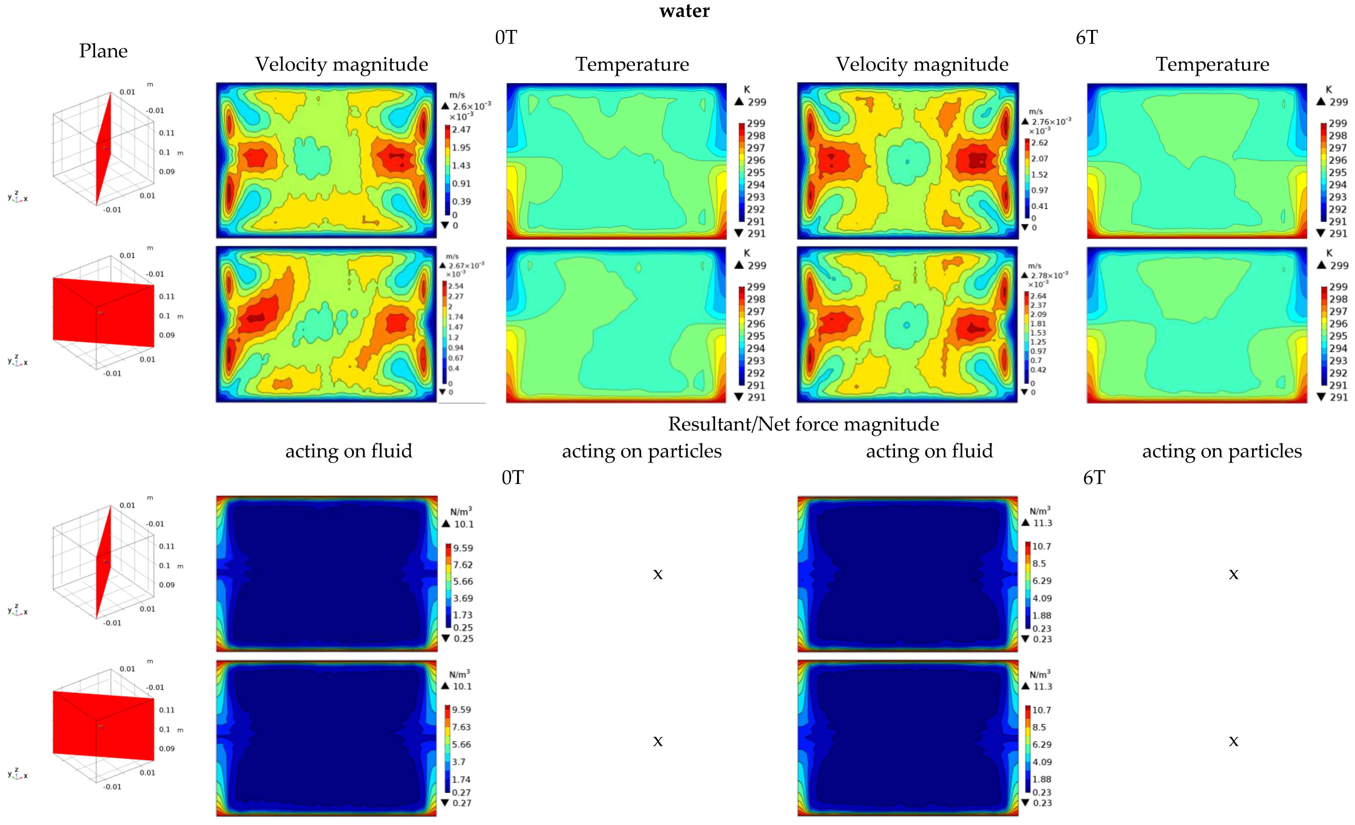
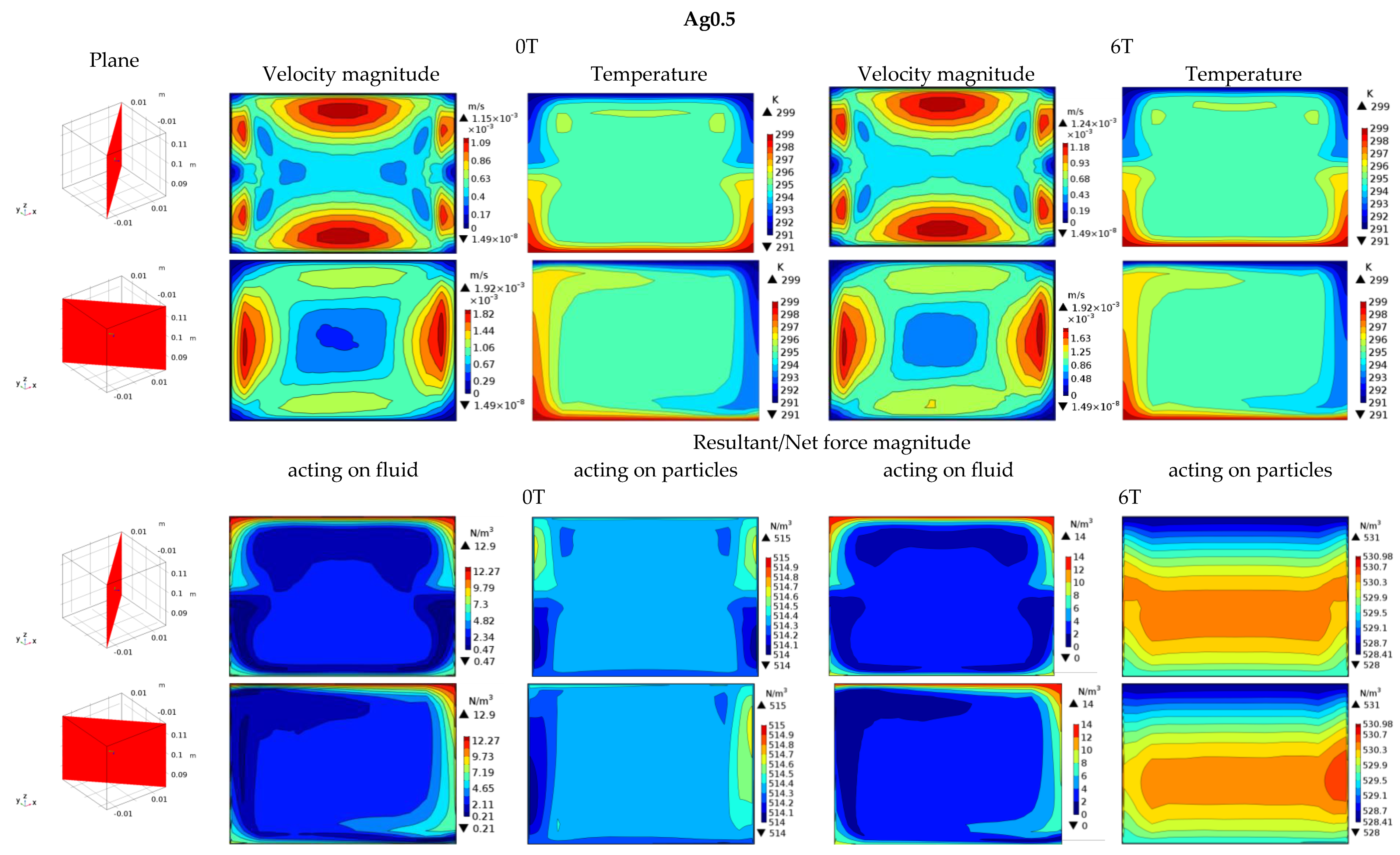
Figure 5 are arranged in the following manner: at the top a kind of fluid is marked, then the velocity magnitude and temperature distributions in two indicated diagonal cross-sections are shown at 0T and 6T of magnetic induction; the bottom part of the figure is related to the net force magnitude (
Fc) acting on the fluid (carrier phase) and the particles (dispersed phase) also at 0 and 6T of magnetic induction. Attention should be payed to the fact that, in the majority of cases, an individual scale is shown. This was done on purpose to visualize the flow structure. When a uniform scale was used, the fine flow pattern disappeared.
In
Figure 2, the results for water are presented. Velocity distribution does not present a typical convection roll at 0 T of magnetic induction. It exhibits streams of higher velocity, in the middle part, which seem to be related to the stream of higher temperature moving up and also the streams of cold fluid flowing down. Interaction between these streams resulted in non-symmetrical structure of the flow. Application of magnetic induction equal to 6T causes change in the velocity magnitude, increasing it slightly in the central part and making its distribution symmetrical. Looking at the net force, the highest value of its magnitude was close to the horizontal walls. When the magnetic field is acting, additional force is added to the system and the magnitude of net force increases.
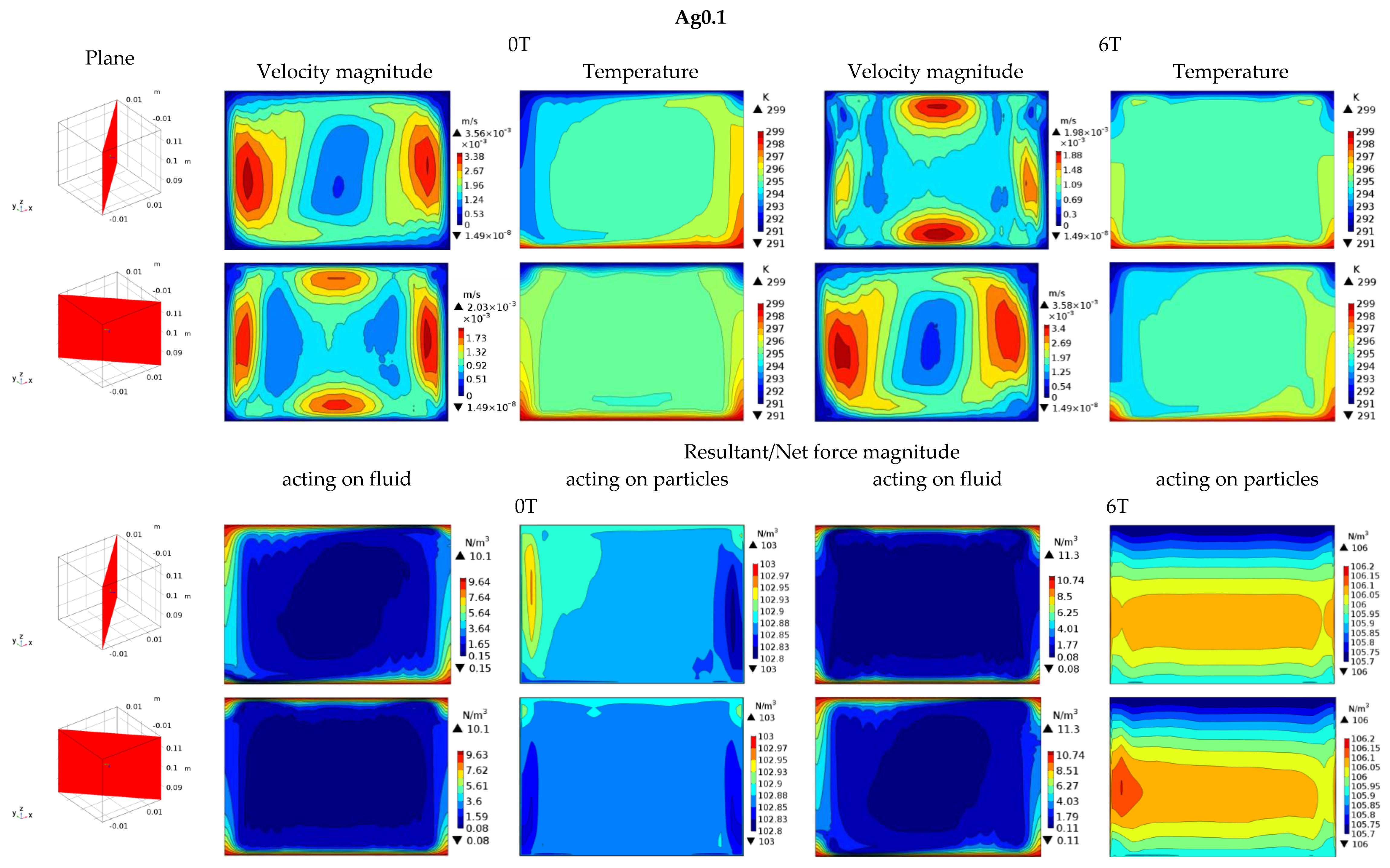
In
Figure 3, the results for nanofluid Ag0.1 are shown. The velocity magnitude distribution suggests one big roll in the enclosure and the areas of high velocity are close to the side walls, along which the streams of cold nanofluid (left side) and hot nanofluid (right side) flow. Influence of the magnetic field of magnetic induction equal to 6T causes the rotation of the flow and the velocity magnitude distribution, in particular for cross-section swaps. By analyzing the distribution of the net force acting on the fluid, it is clear that it is directly connected with temperature distribution and its magnitude takes the highest values in the regions of the highest and the lowest temperature values. Considering the net force acting on the particles, in one cross-section the asymmetry of its magnitude can be seen. On the left side it takes slightly higher values than on the right side. When the magnetic field is applied to the system, the magnitude of the net force acting on the nanofluid changes between the analyzed cross-sections. In the case of particles, the net force magnitude varies horizontally with maximal value in the central part of enclosure.
The results for nanofluid of the highest concentration, namely Ag0.5, are presented in
Figure 5. A very interesting pattern of high and low velocity areas are visible. It suggests few convective rolls present in the enclosure. Application of the magnetic field does not change this pattern, only the value of magnitude slightly increases. A very regular distribution of the net force magnitude acting on the fluid can be found. The highest values are located in the vicinity of the top horizontal (cooled) wall. The biggest influence of magnetic field can be distinguished through the pattern of net force magnitude distribution.
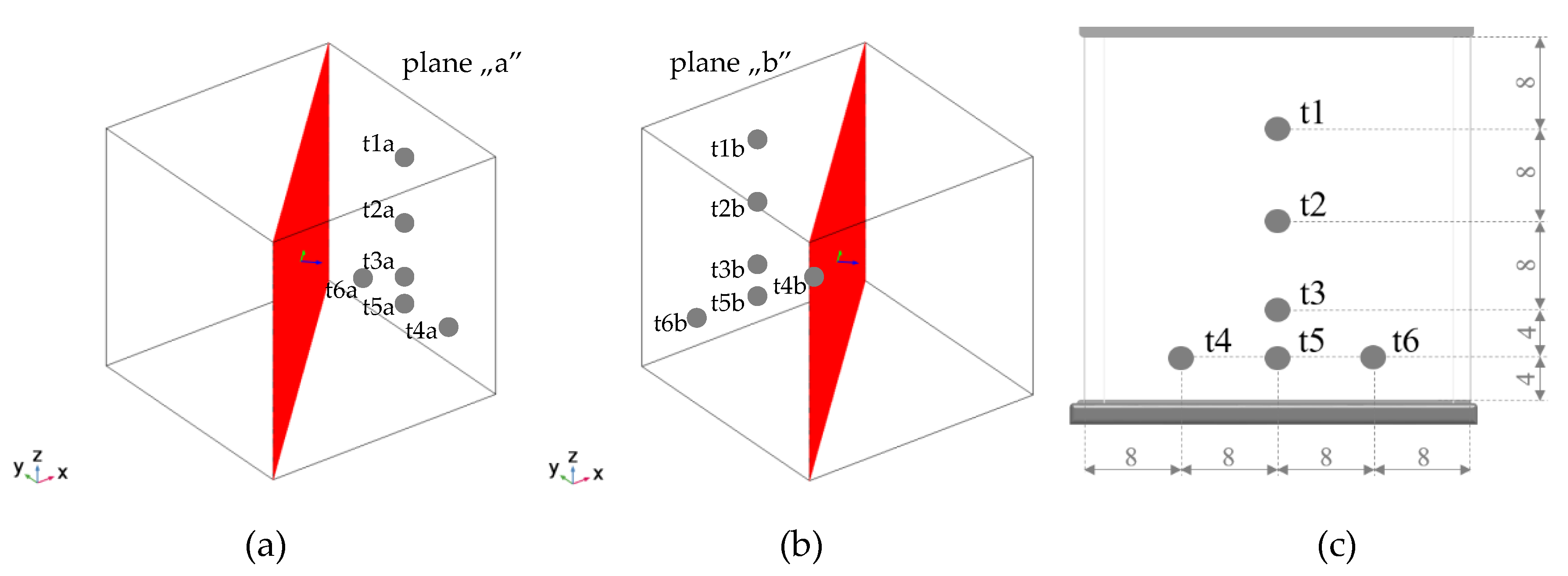
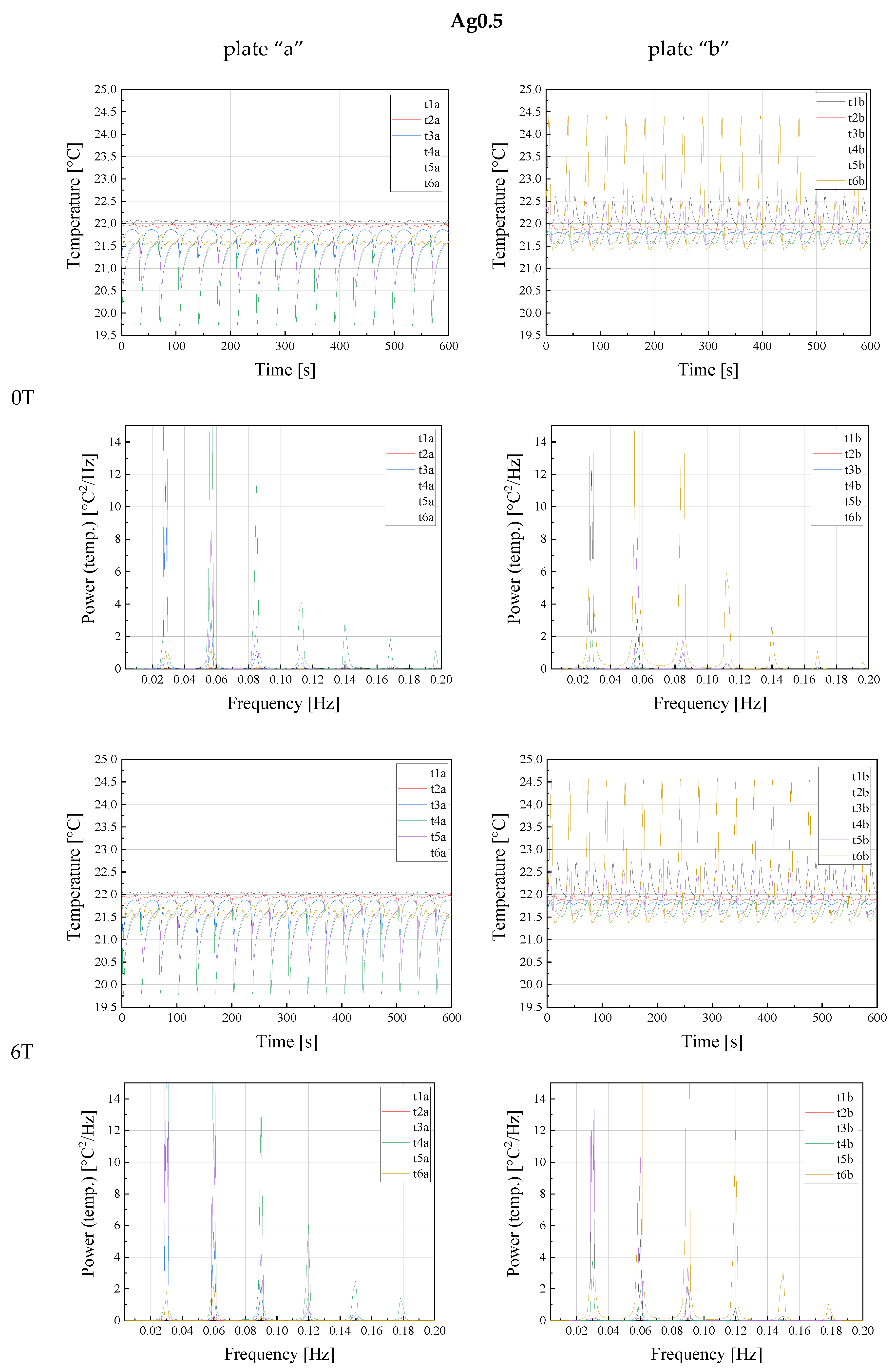
Local values of temperature in the vicinity of two side walls were obtained in the sampling points marked in
Figure 6. Determined temperature values are shown in
Figure 7 and
Figure 8. Six local temperature values during 600 s of convection process are presented at 0 and 6T together with the results of Fast Fourier Transform (FFT). The FFT spectrum through the existence of peaks can suggest the flow structure, combining the peaks of a particular frequency with convective rolls of particular angular speeds. The higher the frequency is, the higher the angular speed of the roll found and the smaller their size.
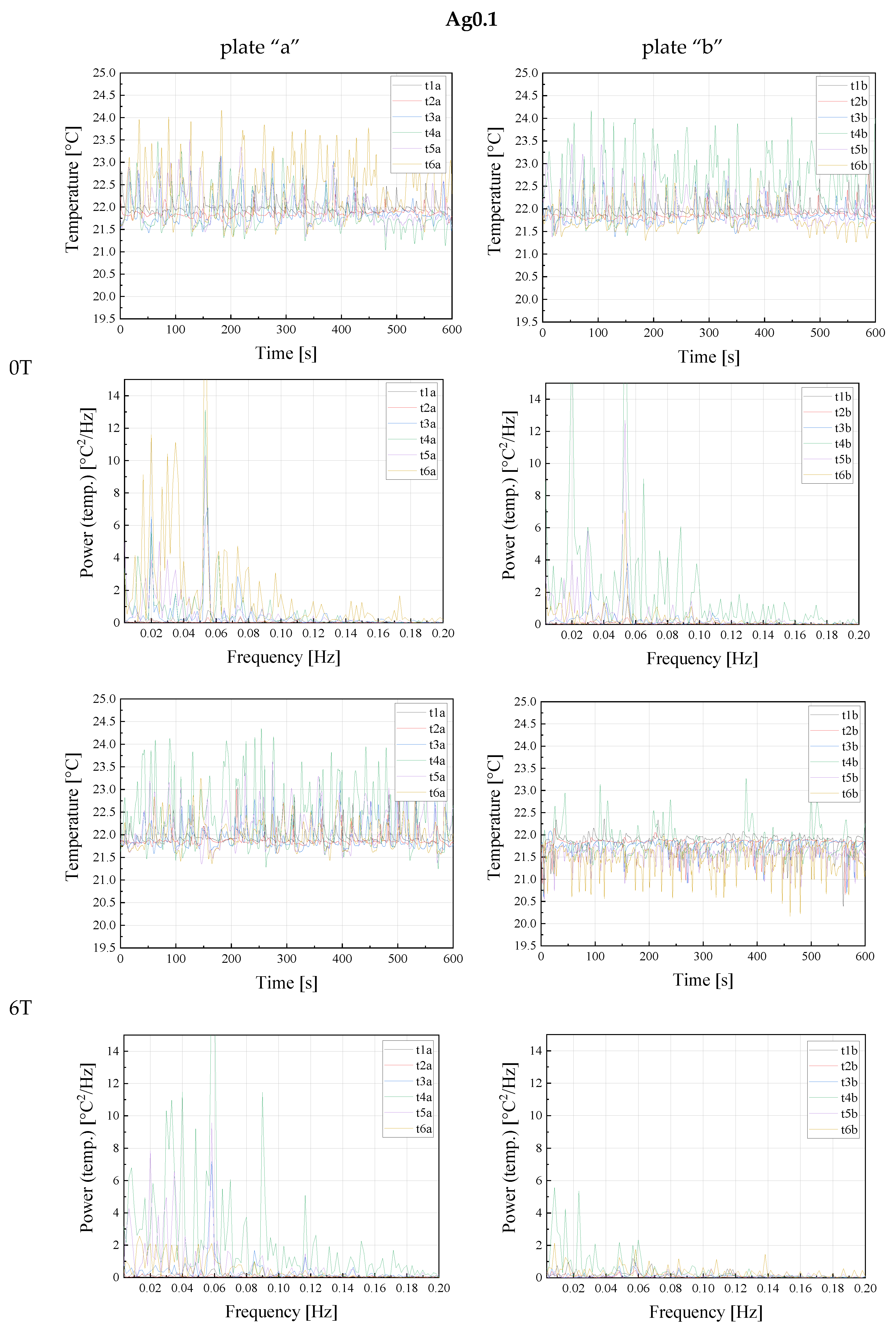
In
Figure 7, the results for the Ag0.1 nanofluid are presented. Instantaneous temperature signals in both planes, “a” and “b”, exhibit fluctuations toward higher temperature values. It suggests movement of the hot stream of the nanofluid. The FFT spectrum is not very clear, but close observation reveals one strong peak of frequency about 0.06 Hz, common for when there are few thermo-couples. It can be understood as a roll of global range. A similar situation is found with the peak of frequency about 0.02 Hz. The other peaks suggest the structure changes with time. Temperature signals at 6T of magnetic induction change their character in plane “a”, the fluctuations are oriented toward the lower temperature values, which indicates movement of cold stream of nanofluid. In plane “b”, the majority of fluctuations become smaller in both directions, which represents area of no direct inflow of any streams on that plane. The FFT spectrum responds to these signals and in plane “a” there is still a peak of frequency of about 0.06 Hz, while one location of sampling points becomes very active. This location is close to the bottom and looks similar to the cold stream of nanofluid reaches that position. Plane “b” is clearly less active and no global roll structure is present. The FFT spectrum corresponds with this swapping of the velocity magnitude distribution, caused by the presence of the magnetic field.
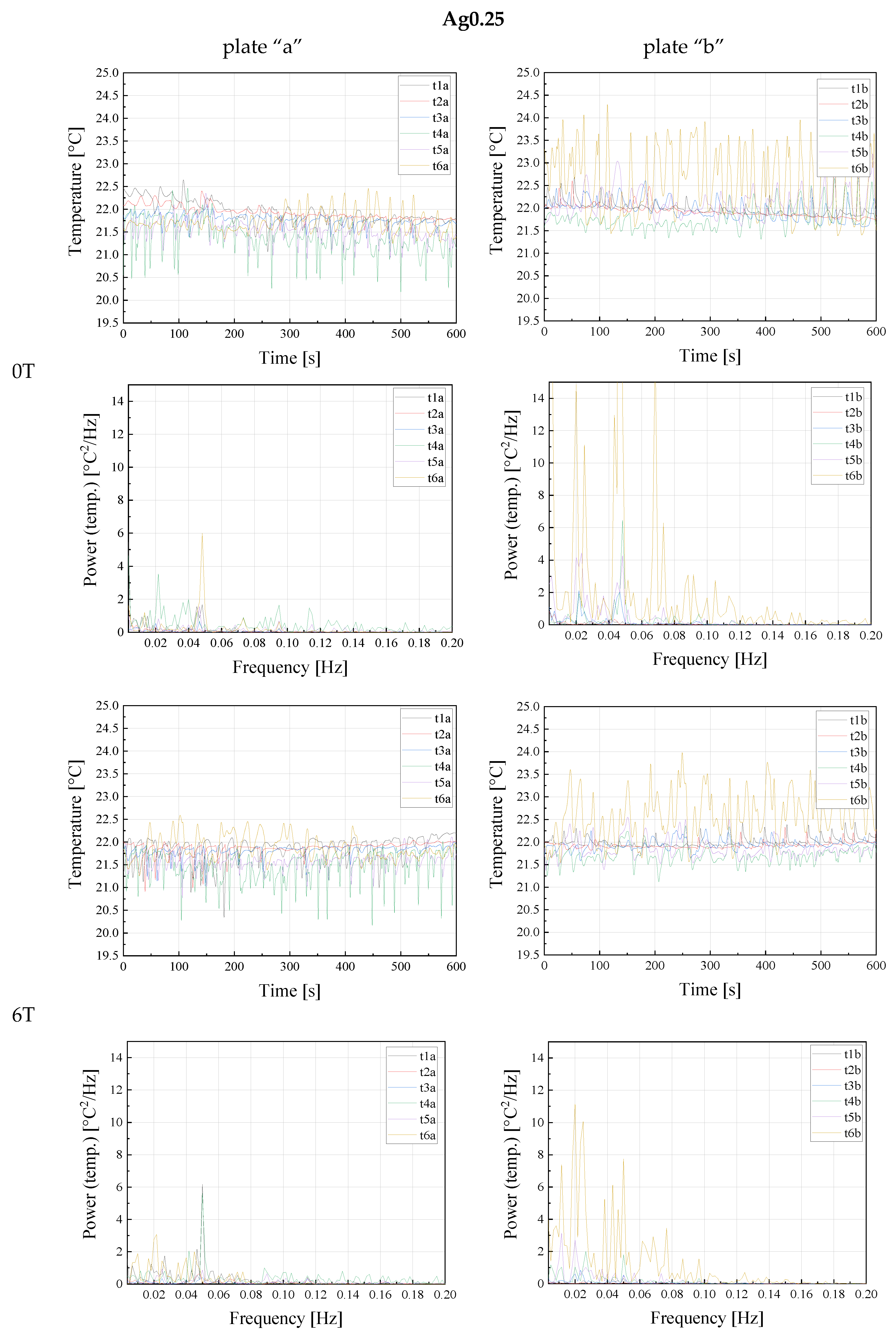
In
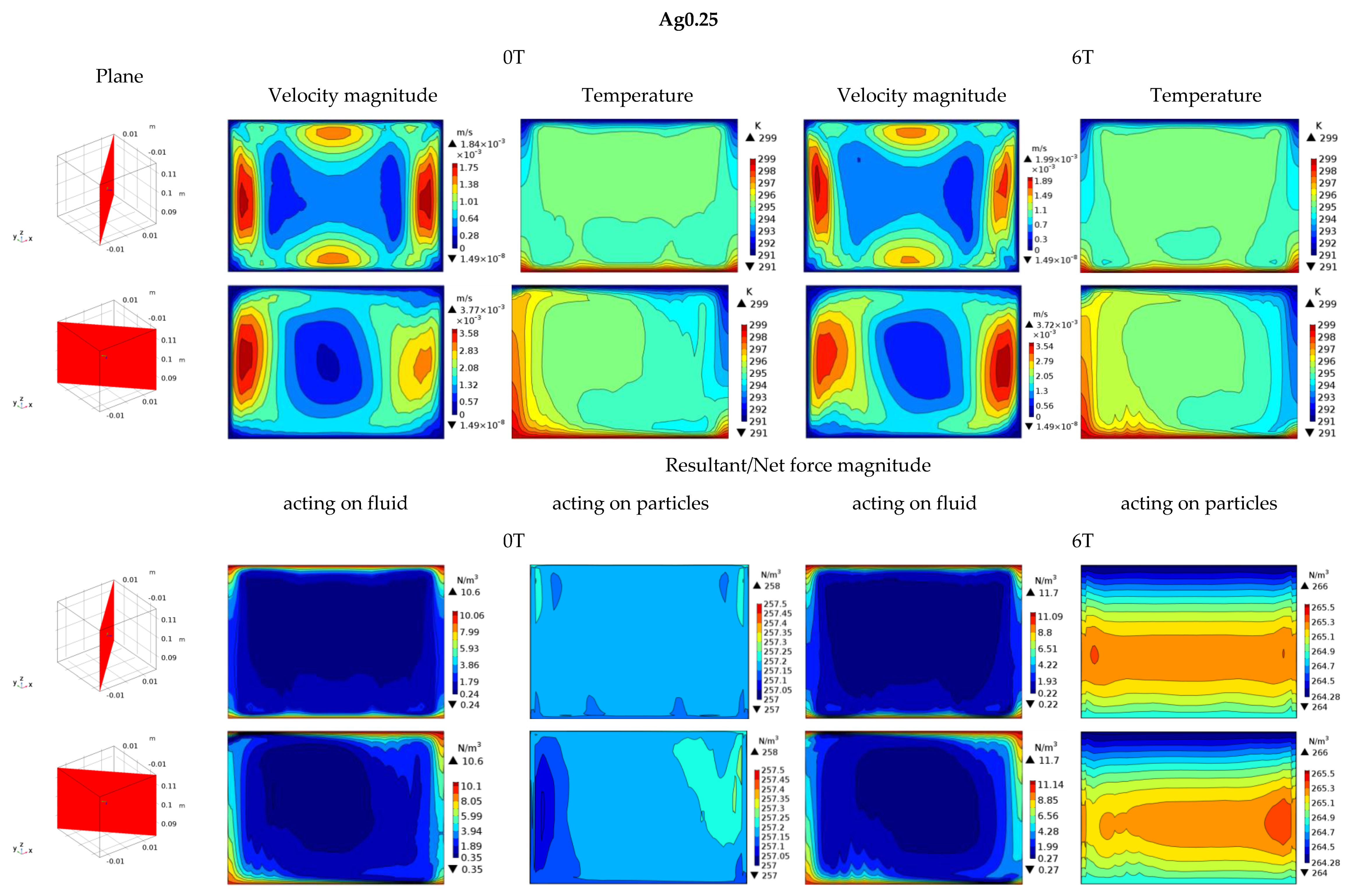
Figure 8, the results for the Ag0.25 nanofluid are presented. In plane “a”, the fluctuations are oriented downwards, what represents downward flow of the cold stream. The power FFT spectrum indicates small peaks of local meaning. There is no global roll in this plane. In plane “b”, high values of temperature fluctuations close to the bottom horizontal are visible, what means that the stream of hot fluid starts to rise. The FFT spectrum exhibits few very high peaks, which might correspond with the flow structure and temperature distribution presented in
Figure 4. At 6T of magnetic induction, there is not much difference in local temperature values in comparison with 0T, and the values seem to be constant in time. The FFT spectrum in the case of plane “a” does not change, but in the case of plane “b” it is characterized by lower peaks values, and it seems to be less clear then at 0T, but it might correspond with the second diagonal, at which some small fluctuations of velocity magnitude and temperature distribution close to the bottom plate are observed.
In
Figure 9, the results for the Ag0.5 nanofluid are presented. Local temperature values demonstrate periodical variations in time. In plane “b”, they represent downward flow of cold streams, while in plane “b” they represent the upward flow of hot ones. The FFT spectrum exhibits seven clearly visible peaks in plane “a” and six in plane “b”, which correspond with the fine pattern of velocity magnitude distribution. The magnetic field of magnetic induction equal to 6T does not change the local temperature values, while the FFT spectrum in the case of plane “a” indicates six peaks. In the case of plane “b”, there are no visible changes.
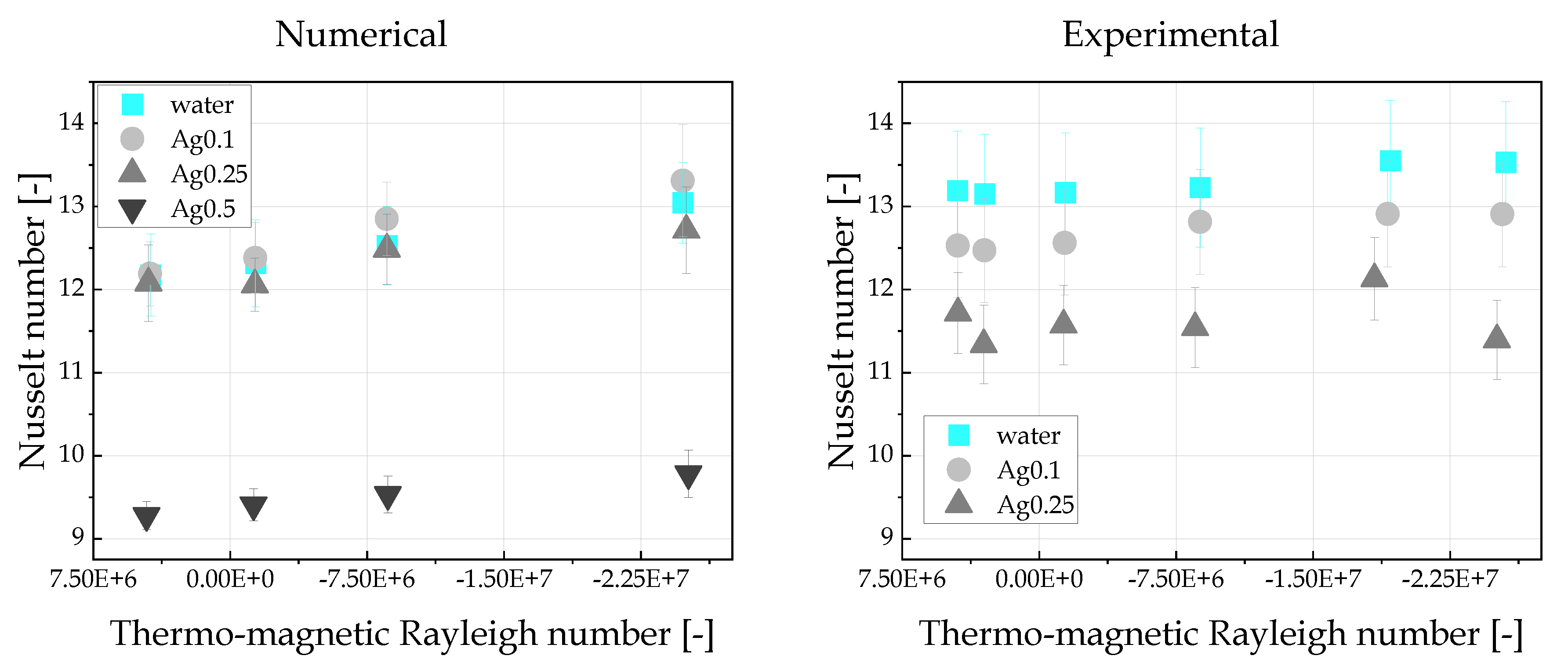
The heat transfer performance of numerically and experimentally analyzed phenomena is presented in
Figure 10 in the form of the Nusselt number value dependence on the thermo-magnetic Rayleigh number defined as:
where Ra
T is the thermal Rayleigh number represented by:
and
γ is the magnetization number expressed as:
g is the gravitational acceleration [m/s
2];
βnf is the thermal expansion coefficient of the nanofluid [1/K] [
27];
ρnf is the density of the nanofuid [kg/m
3];
Cp,nf is the specific heat of nanofluid [J/(kgK)];
μnf is the dynamic viscosity of the nanofluid [kg/(ms)];
knf is the thermal conductivity of the nanofluid [W/(mK)];
d is the characteristic dimension [m]; Δ
T is the temperature difference [K] and
is the magnetic susceptibility determined experimentally [m
3/kg].
The numerically obtained Nusselt number values (
Figure 10, left side) increase with increasing values of thermo-magnetic Rayleigh number in all analyzed cases. However, increasing the concentration of nanoparticles reduces the heat transfer performance. The error bars, indicated in this figure, represent the standard deviation and they can be treated as the uncertainties of the numerical analysis. As discussed above, this tendency was also observed in the experimental analysis described in [
31]. Selected results are shown in
Figure 10 on the right side. The error bars in this figure represent an experimental uncertainty calculated on the basis of error propagation, represented by the variance formula. At lower values of magnetic induction, up to 4T, a small influence of the magnetic field can be recognized. In all experimental cases, it causes attenuation of convection. A magnetic field of magnetic induction ≥6T causes an increase in the Nusselt number value, while the addition of nanoparticles decreases. The most similar results to the numerical ones are the results for water and Ag0.1, both in terms of their tendency and value. A difference between numerical and experimental results can be observed for Ag0.25 at 9T of magnetic induction, but at 10T (not shown here), the value of the Nusselt number increased again. Some discrepancies can be found in the Nusselt number value for the cases without magnetic field. These are the consequence of temperature settings during the experiment, which were very difficult to keep constant. In the case of numerical analysis, such discrepancies can be easily avoided. Taking all mentioned issues into consideration, it can be concluded that an agreement between numerical and experimental analyses is good, especially for such a difficult to experimentally handle medium. Both numerical and experimental results exhibited different tendencies than presented in the literature. Possible reasons come from the analysis of nanofluid flow as two-phase and consideration of momentum exchange between the phases.
6. Discussion
Considering the velocity magnitude of water and nanofluids, it can be observed that, without a magnetic field in some regions, the values were higher for Ag0.1 and Ag0.25 than for water and the smallest was found for Ag0.5. In the case of water, the magnetic field makes the flow symmetrical. It rotates the flow swapping distribution between cross-sections when applied to the Ag0.1 nanofluid. Addition of a magnetic buoyancy force to the system results in preserving the flow structure characteristic for thermal convection of the Ag0.25 nanofluid. A similar situation was observed in the case of the Ag0.5 nanofluid.
The symmetry and asymmetry are both present in the studied phenomena. When the velocity magnitude or temperature distribution are symmetrical, then in the local temperature values asymmetry can be found. In all analyzed cases, symmetry about the diagonal is clearly visible, but another symmetry axis can also be found. The magnetic field definitely stabilizes the flow structure. It should be emphasized, once more, that presented results are averaged over 600 s, so the distributions lasted quite a long time. Obviously, the more intensive convection movement is observed, the less complicated the flow structure is. When the convection motion is slow (as in the case of Ag0.5), more convective rolls appears. All the findings are summarized by the Nusselt number’s dependence on the thermo-magnetic Rayleigh number.
The addition of particles caused a lowering of the Nusselt number, which can be observed in all experimental cases and in the numerical cases of Ag0.25 and Ag0.5. In the numerical case of Ag0.1, another tendency was observed—the averaged Nusselt number was higher than in the case of water. A possible explanation is connected with the low concentration of nanoparticles, which in the magnetic field acts as a promotors of the convection, while the interaction between the phases is negligible. For Ag0.25 and Ag0.5, the momentum transfer between each phase becomes significant, which causes attenuation of convection (lowering of Nusselt number value at 0T of magnetic induction); however, the magnetic buoyancy force helps to overcome it and an increase in the Nusselt number can be observed. This increase is small due to the low values of magnetic susceptibility of the nanofluid components. The flow structure and the heat transfer performance depend on the force systems and their mutual interactions. The gravitational buoyancy force and friction force between the phases are dominant. The magnetic buoyancy force at the analyzed conditions is not strong enough to overcome them, but its presence was noticed. The analysis of higher concentrations of nanoparticles might be of great interest in this matter.


