A Modified Whale Optimization Algorithm with Single-Dimensional Swimming for Global Optimization Problems

Abstract

As a novel meta-heuristic algorithm, the Whale Optimization Algorithm (WOA) has well performance in solving optimization problems. However, WOA usually tends to trap in local optimal and it suffers slow convergence speed for large-scale and high-dimension optimization problems. A modified whale optimization algorithm with single-dimensional swimming (abbreviated as SWWOA) is proposed in order to overcome the shortcoming. First, tent map is applied to generate the initialize population for maximize search ability. Second, quasi-opposition learning is adopted after every iteration for further improving the search ability. Third, a novel nonlinearly control parameter factor that is based on logarithm function is presented in order to balance exploration and exploitation. Additionally, the last, single-dimensional swimming is proposed in order to replace the prey behaviour in standard WOA for tuning. The simulation experiments were conducted on 20 well-known benchmark functions. The results show that the proposed SWWOA has better performance in solution precision and higher convergence speed than the comparison methods.

1. Introduction

With the development of technology, increasing global optimization problems have to be solved in various fields, such as economic scheduling, aerospace, signal processing, artificial intelligence, mechanical design, chemical engineering [1,2,3], etc. In general, optimization problems with typical mathematical characteristics can be solved by traditional algorithms and the optimal solution is guaranteed in this case. However, many problems in modern applications have the characteristics of large-scale, high-dimensional, and lack of typical mathematical characteristics, and they cannot be solved by traditional optimization algorithms or the solution is too complex to be feasible. For this, many scholars have conducted research on the meta-heuristic algorithm and have remarkable results.

A meta-heuristic algorithm is an implementation on a specific problem guided by a set of guidelines or strategies, which adopts the “trial-and-error” mechanism [4]. The “trial-and-error” mechanism is a method for obtaining a feasible solution at first, and then gradually improve it by comparing the fitness of feasible solutions, finally approach or obtain the optimal solution. The meta-heuristic algorithms cannot guarantee to obtain the optimal, but it can obtain a satisfactory solution within a certain amount of time. The “trial-and-error” mechanism adopted by the meta-heuristic algorithms ensure that it does not require the problem to have precise mathematical characteristics, and it is very adaptable. Motivated by the diversity of engineering applications, many meta-heuristic algorithms have been proposed, such as the Genetic Algorithm (GA) [5,6], Simulated Annealing (SA) [7,8], and the subsequently, Ant Colony Optimization (ACO) [9,10], Differential Evolution (DE) [11], Particle Swarm Optimization (PSO) [12,13,14], Gravitational Search Algorithm (GSA) [15], and so on. Some of these meta-heuristic algorithms are called Swarm Intelligent algorithm (SI), which iteratively solve problems by simulating group collaboration. In recent years, a large number of novel swarm intelligent optimization algorithms have been proposed in order to meet the challenge of global optimization problems, such as artificial bee colony optimization (ABC) [16,17,18], Whale Optimization Algorithm, (WOA) [19,20,21,22], Glowworm Swarm Optimization (GSO) [23,24], Grey Wolf Optimization (GWO) [25], and Symbiotic Organisms Search (SOS) [26,27], etc.

The meta-heuristic algorithm can generally obtain good results when solving small-scale optimization problems, but, when targeting some high-dimensional large-scale optimization problems, there are often two problems: (1) convergence speed slow, which leads to long computation time; and, (2) it is easy to fall into the local optimum. These two problems are related to each other, the former is that the approximation speed is too low, which can be improved by improving some parameters or introducing some mechanisms, while the latter is mainly due to the lack of population diversity, which is directly related to the final solution quality, and it can be improved by enhancing population diversity. Many scholars have conducted a lot of work on the shortcomings of meta-heuristic algorithms, and have obtained good results by improving the standard algorithm or mixing the standard algorithm with various mechanisms.

Whale Optimization Algorithm is a new meta-heuristic optimization algorithm for simulating humpback whale hunting behavior proposed by Mirjalili [28] in 2016, and it has been shown that WOA has better optimization performance when compared to PSO, ABC, and DE algorithms [29], but it still suffers from slow convergence and low solution accuracy when solving high-dimensional large-scale optimization problems. In view of this, a lot of work has been done on WOA for improving the WOA algorithm in order to obtain better performance. In the literature [30], Adel introduces the concept of leader to guide the population into the optimal solution region, which enhances the convergence speed of WOA. In [31], Mohamed proposed that chaotic sequences and Opposition-Based Learning (OBL) are the two most effective ways to improve WOA. The adaptive chaotic sequence selection method is proposed in the paper in order to improve the diversity of the initial population and, at the same time, a part of the population is selected to execute the DE algorithm, which finally results in an improved DEWCO algorithm that is a mixture of WOA and DE. A nonlinear dynamic control parameter update strategy that is based on a cosine function is proposed in [20] in order to balance the exploration and tuning ability. Additioanlly, the Lévy flight strategy is used to make the algorithm jump out of the local optimum and avoid stagnation [22]. In the literature [19], a WOA based on quadratic interpolation is proposed. The algorithm mainly introduces new parameters, improves the search process, and balances the convergence speed and solution accuracy. At the same time, quadratic interpolation is used to search the optimal agent, which improves the solution accuracy. The literature [21] employs a logistic chaos map in order to improve the distribution of the initial population in the solution space and a quasi-opposition learning mechanism, in which both the standard algorithm and the quasi-opposition learning generate and evaluate agents during predation, and the better agent is retained by comparing the adaptation values of the two agents to improve the convergence speed. In literature [32], two strategies are used to improve the standard WOA: (1) random replacement of poorer agents with better ones, which is used to improve the algorithm’s solution convergence speed, and (2) adaptive double weights, which is used to balance the algorithm’s early spatial search ability and later local spatial tuning ability. There are three main improvements in the literature [33]; firstly, a chaotic sequence is introduced for optimizing the initial population. Subsequently, Gaussian variation is used to maintain the diversity level of the population. Finally, a “reduced” strategy is used to search near the optimal solution. The literature [34] introduced quantum behavior in the standard WOA to simulate the hunting process of humpback whales in order to enhance the search capability of the algorithm, which is used for feature selection. Although these studies have improved the standard WOA algorithm to some extent, there are still problems of slow convergence and low solution accuracy, especially for high-dimensional large-scale optimization problems.

In this paper, a modified WOA algorithm SWWOA based on single-dimensional swimming is proposed, with four main improvements: (1) the use of tent chaotic sequences to optimize the quality of the initial population; (2) the introduction of quasi-opposition learning mechanism, any agent updated position will be learned by quasi-opposition learning, retain the better agent by fitness; (3) the use of logarithmic function to dynamically update the weights, instead of the original linear weights. Balancing the between convergence speed and solution quality; and, (4) the single-dimensional swimming improvement is borrowed from the single-dimensional update of position in the ABC algorithm, which replaces the full dimensional update in the standard WOA with single-dimensional improvement in order to further improve the algorithm’s ability.

The rest of paper is organized, as follows. Section 2 introduces the standard whale optimization algorithm. Section 3 describes the proposed SWWOA algorithm. Simulations and the discussion of results are shown in Section 4. Finally, Section 5 gives the conclusions.

2. Standard WOA Algorithm

WOA is a novel meta-heuristic optimization algorithm by imitating the hunting mechanism of humpback whales, which consists of three phases: encircling prey, spiral bubble-net feeding maneuver, and search for prey [28].

2.1. Encircling Prey (Exploitation Phase)

At this stage, the algorithm sets the current optimal position in the population as the global optimal, which is, the prey. All of the whales in the population move towards the prey and gradually shrink to surround the prey, as follows:

$$\overrightarrow{D}=\left|C·\overrightarrow{X^{*}}\left(t\right)-\overrightarrow{X}\left(t\right)\right|$$

(1)

$$\overrightarrow{X}\left(t+1\right)=\overrightarrow{X^{*}}\left(t\right)-A·\overrightarrow{D}$$

(2)

where t represents the current time, $\overrightarrow{X}$ is the position vector, which represents a feasible solution. $\overrightarrow{X^{*}}$ represents the optimal solution at the current time and $\left|·\right|$ represents the absolute value. A and C are two control parameters, which are calculated, as follows:

$$A=2ar-a$$

(3)

$$C=2r$$

(4)

where a is linearly factor from 2 to 0 over the whole iterations (both exploration and exploitation) and r is a random number in [0, 1].

2.2. Bubble-Net Attacking Method (Exploitation Phase)

At this stage, WOA imitate humpback whales attacking prey with bubble net, which are essentially spiral search space, whose mathematical model is as follows:

$$\overrightarrow{D^{\prime }}=\left|\overrightarrow{X^{*}}\left(t\right)-\overrightarrow{X}\left(t\right)\right|$$

(5)

$$\overrightarrow{X}\left(t+1\right)=\overrightarrow{D^{\prime }}·e^{bl}·\cos \left(2\pi l\right)+\overrightarrow{X^{*}}\left(t\right)$$

(6)

where $\overrightarrow{D^{\prime }}$ represents the distance between current whale and the best solution of population. l is a random number in [−1, 1] and b is a constant used in order to define the shape of the spiral, normally is 1. Exploitation phase has bubble-net attacking and encircling prey two methods, each is implemented with 50% probability. Accordingly, combining the two method, the following formula can be obtained:

$$\overrightarrow{X}\left(t+1\right)=\left\{\begin{array}{cc}\overrightarrow{X^{*}}\left(t\right)-A·\overrightarrow{D}& p<0.5\\ \overrightarrow{X^{*}}\left(t\right)+\overrightarrow{D^{\prime }}·e^{bl}·\cos \left(2\pi l\right)& p\ge 0.5\end{array}\right.$$

(7)

2.3. Search for Prey (Exploration Phase)

In a standard WOA algorithm, this stage is the mainly phase for exploration, where the mathematical model is similar to Equations (1) and (2), and the only difference is the use of a random agent instead of the optimal agent. The formula is as follows:

$$\overrightarrow{D}=\left|C·\overrightarrow{X_{rand}}\left(t\right)-\overrightarrow{X}\left(t\right)\right|$$

(8)

$$\overrightarrow{X}\left(t+1\right)=\overrightarrow{X_{rand}}\left(t\right)-A·\overrightarrow{D}$$

(9)

$\overrightarrow{X_{rand}}$ denotes a random agent in population, other meanings same to the Section 2.1. It is worth noting that the scheduling between encircling (exploitation) and search (exploration) is done by the value of $\left|A\right|$. When $\left|A\right|<1$, exploitation is selected. When $\left|A\right|\ge 1$, exploration is selected.

2.4. The Pseudo Code of WOA

When compared with other meta-heuristic algorithms, in addition to the necessary parameters, such as population size and max iteration times, the WOA algorithm only has one parameter a for balanced exploitation and exploration, which is a very good advantage. However, from another aspect, WOA has very few adjustable parameters and it is slightly lacking in flexibility. The pseudo code of the standard WOA Algorithm 1 is as follows:

Algorithm 1 WOA

01 initialize maxIteration, popsize and parameter b 02 initialize the population and calculate fitness 03 obtain the optimal agent 04 WHILE t<maxIteration DO 05  update a, A, C by Equations (3) and (4) 06  WHILE i<popsize DO 07   generate random number $p\in [0,1]$ 08   IF p < 0.5 THEN 09    IF $\left|A\right|<1$ THEN 10     update position of agent i by Equation (2) 11    ELSE 12     generate random agent rand 13     update position of agent i by Equation (9) 14    ENDIF 15   ELSE 16     update position of agent i by Equation (6) 17   ENDIF 18   i = i + 1 19  ENDWHILE 20  update optimal agent if there is a better solution 21   t = t + 1 22 ENDWHILE 23 RETURN optimal agent

3. Whale Optimization Algorithm with Single-Dimensional Swimming (SWWOA)

In this paper, an improved algorithm is proposed for the features of the standard WOA algorithm. The main improvements are divided into four interrelated aspects. First, the quality of the initial population is directly related to the convergence speed and, if there are agents located in the optimal solution region at the beginning, it will save a lot of useless calculations. Subsequently, quasi-opposition learning is introduced in order to improve search capability in all directions. On the basis of greatly improving the search ability, this paper introduces a logarithm-based nonlinear parameter, which is used in order to apply more computation to tuning and improve the solution accuracy. Finally, borrowing from the ABC algorithm for finding food, the full-dimensional encircling prey is replaced by a single-dimensional swimming, which is essentially a more fine-grained approach to finding excellence and, moreover, gives the algorithm the ability to jump out of the local optimum. Before describing the improvements in this paper, the test functions are first described.

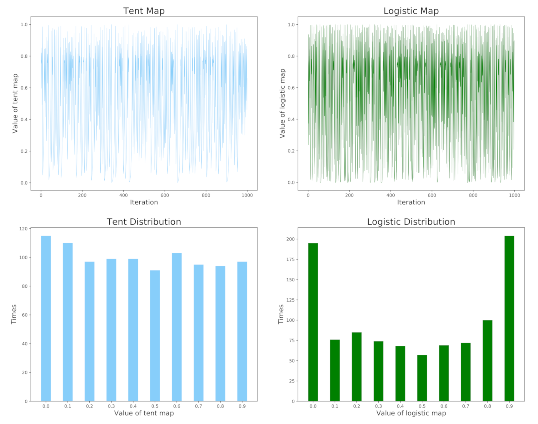
3.1. Chaotic Sequence Based on Tent Map

A chaotic system is a deterministic system, in which there is seemingly random irregular movement that behaves in an indeterminate, unrepeatable, and unpredictable manner [21]. Chaos is an inherent property of nonlinear system and it is a common phenomenon in nonlinear systems. There are many map functions for chaotic system, the most commonly used of which are logistic map and tent map [21,31,33]. In this paper, we use tent map with the following formula. Presently, most of the improved algorithms use logistic map. However, logistic map has uneven traversal characteristics, while tent map has better uniform characteristics [31]. Figure 1 shows the specific comparison of logistic map and tent map.

In this paper, the tent map is selected, whose formula is as follows:

$$s_{k+1}=\left\{\begin{array}{cc}10s_k/7& s_k<0.7\\ 10(1-s_k)/3& s_k\ge 0.7\end{array}\right.$$

(10)

when the initial value $s_1\in \left(0,1\right)$ is randomly given, through Equation (10) iteration $n-1$ times, a chaotic sequence $\left\{s_{1,}{s}_2,\cdots ,s_n\right\}$ can be generated. The initial agent can be generated by mapping the sequence to the solution, as follows:

$$x_i=x_{i,\min }+(x_{i,\max }-x_{i,\min })s_i$$

(11)

where $x_{i,\min }$ represents the lower boundary of x in the i-th dimension, $x_{i,\max }$ represents the upper boundary of x in the i-th dimension. At the time of initialization, all of the agents in the population are mapping according to formula Equations (10) and (11) in order to generate chaotic population.

3.2. Quasi-Opposition Learning

In the meta-heuristic algorithm, feasible solutions are obtained first, and then the solution space is searched for the optimal based on the fitness of the feasible solution. Various different meta-heuristic algorithms search in different ways, but all of them essentially have a random factor. In recent years, Opposition-Based Learning [35] has been widely used in meta-heuristic algorithms [21,27,29], which is essentially a method of replacing random search with symmetric search, which can greatly improve the search ability of the algorithm.

Although the opposite-learning method improves the search capability of the algorithm considerably, Opposition-Based Learning is too fixed and not very effective for tuning in a small space. The literature [31,36] proposes quasi-opposite learning, which adds a random factor to Opposition-Based Learning, and the resulting position is not a fixed symmetric position, but a random position between the central position and the symmetric position. Assuming $x\in [a,b]$, the expression for quasi-opposite learning is as follows:

$$x^o=\frac{a+b}{2}+r\left(\frac{a+b}{2}-x\right)$$

(12)

where $r\in [0,1]$ is a random variable. If $r\in [0,2]$, quasi-opposite point theoretically has 50% chance falling within the symmetry point and the center, and 50% chance of falling outside the symmetry point. If it falls within the symmetry point, it is good for algorithm tuning to improve solution quality, while falling outside the symmetry point is more good for spatial search to improve convergence speed. If the variables x are multi-dimensional, then each dimension of x needs to separately execute Equation (12), i.e., where a and b are vectors, the multi-dimensional expression is as follows:

$$\overrightarrow{x^o}=\frac{\overrightarrow{a}+\overrightarrow{b}}{2}+r\left(\frac{\overrightarrow{a}+\overrightarrow{b}}{2}-\overrightarrow{x}\right)$$

(13)

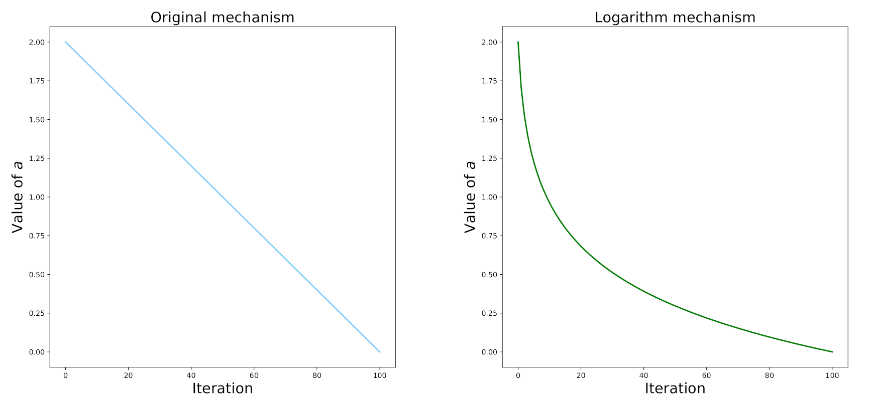
3.3. Logarithm-Based Nonlinear Control Parameter

There is only one control parameter a in the standard WOA, as mentioned in Section 2.3 and Section 2.4. This parameter controls the proportion of exploitation and exploration, as shown in Equation (3). In the standard WOA, the parameter a varies linearly from 2 to 0, while the direct control of exploration and exploitation is $\left|A\right|$. From Equation (3) alone, exploration and exploitation each account for about 50% weight. At the beginning of WOA, exploration accounts for a greater proportion and, after beginning, the proportion of exploration gradually decreases, while that of exploitation gradually increases.

The proposed SWWOA algorithm, employs a chaos mechanism Section 3.1 and quasi-opposite learning Section 3.2 mechanism, which has already improved exploration more substantially, so nonlinear control mechanism based on logarithm with a greater proportion of exploitation is employed, which improves the tuning ability of the algorithm and ultimately improves the quality of the solution. The expression of parameter is as follows, and the comparison of two parameter mechanism is shown in Figure 2:

$$a=2-{log}_{10}\left(1+\frac{99t}{t_{\max }}\right)$$

(14)

where t denotes t-th iteration, $t_{\max }$ denotes the max iteration times. As can be seen in Figure 2, the logarithm-based control parameter curve starts out very steep and declines rapidly, while it flattens out later. Overall, the tuning is performed with greater probability.

3.4. Single-Dimensional Swimming

It has been documented in [16], that the ABC algorithm has better optimization performance when compared with algorithms, such as PSO and GA. Most of the above improvements in this paper are dedicated to improving the search capability, in order to allow for the population to perform a fine-grained search in a narrow space near the optimal; this paper introduces the employed bee position update method in the ABC algorithm for single-dimensional swimming.

$$D_d=\left|C·X_d^{*}\left(t\right)-X_d\left(t\right)\right|$$

(15)

$$X_d\left(t+1\right)=X_d^{*}\left(t\right)-A·D_d$$

(16)

where d denotes a dimension, randomly generated for each agent, otherwise refer to Equations (1) and (2).

3.5. The Pseudo Code of SWWOA

SWWOA introduces four improvements to the standard WOA. These four improvements are interrelated. Chaos mechanisms and opposition-based learning are used in order to improve the spatial search capability; on top of this, nonlinear control parameter factors are introduced, which are used to apply more computations to tuning, and finally single-dimensional swimming are used inn order to search in narrow space and improve the solution quality. In Section 4, the ablation experiment is designed to discuss the impact of each improvement on the algorithm. The pseudo code of the standard SWWOA Algorithm 2 is as follows:

Algorithm 2 SWWOA

01 initialize maxIteration, popsize and parameter b 02 initialize chaos population and calculate fitness by Equations (10) and (11) 03 obtain the optimal agent 04 WHILE t<maxIteration DO 05  update a by Equation (14) 06  update A, C by Equations (3) and (4) 07  WHILE i<popsize DO 08   quasi-opposition learning $x_i^o$ on agent i by Equation (13) 09   generate random number $p\in [0,1]$ 10   IF p < 0.5 THEN 11    IF $\left|A\right|<1$ THEN 12     generate random dimension d 13     update position of agent i by Equations (15) and (16) 14    ELSE 15     generate random agent rand 16     update position of agent i by Equation (9) 17    ENDIF 18   ELSE 19    update position of agent i by Equation (6) 20   ENDIF 21   compare $x_i^o$ and $x_i$, retaining the better agent 22   i = i + 1 23  ENDWHILE 24  update optimal agent if there is a better solution 25  t = t + 1 26 ENDWHILE 27 RETURN optimal agent

4. Experimental Results and Analysis

In order to verify the effectiveness of the proposed algorithm, we select other four algorithms (WOA [28], ABC [16], PSO [12], and OBCWOA [21]) to conduct comparative experiments on 20 well-known test functions. The language used for the implementation is C/C++, the compiler is gcc-4.8.5, the computer CPU is i3-9100, the memory is 16GB, and the CentOS-7.5 amd64 with kernel 3.10 operating system is used.

The PSO algorithm is a very famous meta-heuristic algorithm, which has a very stable performance and it is often used as a benchmark for meta-heuristic algorithm. The ABC algorithm is also a much studied algorithm with high solution quality, which is selected in this paper, because SWWOA draws on its scout bee update mechanism. SWWOA is a proposed algorithm based on standard WOA, and the standard WOA is also selected. In addition, the literature [21], which is almost the latest improvement algorithm of the standard WOA, it uses a chaos mechanism and quasi-opposition learning mechanism, which is similar to SWWOA, so the OBCWOA algorithm proposed in [21] is selected. Among the above four algorithms, ABC is special, in that it is mainly updated in single-dimensional way. For fairness, more iterations and a bigger population size are set for ABC.

Table 1. Parameter setting.

Algorithm	Parameter Settings
ABC	$popsize=60$, $t_{\max }=2000$, $trial=20$
PSO	$popsize=30$, $t_{\max }=1000$, $w=0.9-(0.9-0.2)t/t_{\max }$,
	$c_1=1.5$, $c_2=1.5$, $V\in [-0.5,0.5]$
WOA	$popsize=30$, $t_{\max }=1000$, $a=2\left(1-t/t_{\max }\right)$,
OBCWOA	$popsize=30$, $t_{\max }=1000$, $a=2\left(1-t/t_{\max }\right)$, $a_{logistic}=4$, $b=1$
SWWOA	$popsize=30$, $t_{\max }=1000$, $a=2-{log}_{10}\left(1+99t/t_{\max }\right)$, $b=1$

shows the specific parameters of algorithm.

4.1. Test Functions

A series of large-scale and high-dimensional test functions presented in

Table 2. Test functions.

Name	Equation	Range	Type
Sphere	$f_1\left(x\right)={\sum }_{i=1}^n{x}_i^2$	${[-100,100]}^n$	US
Sum Squares	$f_2\left(x\right)={\sum }_{i=1}^{n}i{x}_i^2$	${[-10,10]}^n$	US
Schwefel 2.21	$f_3\left(x\right)=\max \left|x_i\right|,1\le i\le n$	${[-100,100]}^n$	US
Powell Sum	$f_4\left(x\right)={\sum }_{i=1}^n|x_i{|}^{i+1}$	${[-1,1]}^n$	US
Quartic	$f_5\left(x\right)={\sum }_{i=1}^{n}i{x}_i^4$	${[-1.28,1.28]}^n$	US
Step	$f_6\left(x\right)={\sum }_{i=1}^n{⌊x_i+0.5⌋}^2$	${[-100,100]}^n$	US
Zakharov	$f_7\left(x\right)={\sum }_{i=1}^n{x}_i^2+({\sum }_{i=1}^{n}0.5i{x}_i{)}^2+({\sum }_{i=1}^{n}0.5ix{)}^4$	${[-5,10]}^n$	UN
Rosenbrock	$f_8\left(x\right)={\sum }_{i=1}^{n-1}[100{(x_{i+1}-x_i^2)}^2+{(x_i-1)}^2]$	${[-30,30]}^n$	UN
Schwefel 1.2	$f_9\left(x\right)={\sum }_{i=1}^n{\left({\sum }_{j=1}^i{x}_j\right)}^2$	${[-100,100]}^n$	UN
Schwefel 2.22	$f_{10}\left(x\right)={\sum }_{i=1}^n|x_i|+{\prod }_{i=1}^n\left|x_i\right|$	${[-10,10]}^n$	UN
Discus	$f_{11}\left(x\right)={10}^6{x}_1^2+{\sum }_{i=2}^n{x}_i^6$	${[-1,1]}^n$	UN
Cigar	$f_{12}\left(x\right)=x_1^2+{10}^6{\sum }_{i=2}^n{x}_i^6$	${[-100,100]}^n$	UN
Alpine	$f_{13}\left(x\right)=\left|x_{i}sin\left(x_i+0.1x_i\right)\right|$	${[-10,10]}^n$	MS
Rastrigin	$f_{14}\left(x\right)={\sum }_{i=1}^n(x_i^2-10cos2\pi x_i+10)$	${[-5.12,5.12]}^n$	MS
Bohachevsky	$f_{15}\left(x\right)={\sum }_{i=1}^{n-1}(x_i^2+2x_{i+1}^2-0.3cos3\pi x_i-0.4cos4\pi x_{i+1}+0.7)$	${[-50,50]}^n$	MS
Griewank	$f_{16}\left(x\right)={\sum }_{i=1}^n{x}_i^2/4000-{\prod }_{i=1}^{n}cos(x_i/\sqrt{i})+1$	${[-60,60]}^n$	MN
Weierstrass	$f_{17}\left(x\right)={\sum }_{i=1}^n{\sum }_{k=0}^{20}\{[cos\left(2\pi 3^k(x_i+0.5)\right)-cos(2\pi 3^k·0.5)]/2^k\}$	${[-0.5,0.5]}^n$	MN
Ackley	$f_{18}\left(x\right)=-20exp(-0.2\sqrt{\frac{{\sum }_{i=1}^n{x}_i^2}{n}})-exp{\sum }_{i=1}^n\frac{cos2\pi x_i}{n}+20+e$	${[-32,32]}^n$	MN
Schaffer	$f_{19}\left(x\right)=0.5+[{sin}^2{\left({\sum }_{i=1}^n{x}_i^2\right)}^{0.5}-0.5]/{(1+{\sum }_{i=1}^n{x}_i^2/1000)}^2$	${[-100,100]}^n$	MN
Salomon	$f_{20}\left(x\right)=1-cos\left(2\pi \sqrt{{\sum }_{i=1}^n{x}_i^2}\right)+\sqrt{{\sum }_{i=1}^n{x}_i^2}/10$	${[-100,100]}^n$	MN

are utilized to test algorithms’ performance. $f_1$–$f_6$ are unimodal-separable functions (abbreviated as US), mainly to check the convergence speed of the algorithm. $f_7$–$f_{12}$ are unimodal-nonseparable functions (abbreviated as UN), when compared with the US functions, more able to detect the search capability of the algorithm. $f_{13}$–$f_{15}$ are multimodal-separable functions (abbreviated as MS), more test algorithm out of the local optimum ability. $f_{16}$–$f_{20}$ are multimodal-nonseparable functions (abbreviated as MN); these types of functions are more complex and more reflective of the overall performance.

4.2. Numerical Analysis

In the comparative experiments, the problem dimensions are set to 20 (

Table 3. Comparison results for 20 test functions with n = 20.

Function		ABC	PSO	WOA	OBCWOA	SWWOA
	best	8.38 $\times {10}^{-07}$	1.29 $\times {10}^{-39}$	1.86 $\times {10}^{-185}$	0.00 $\times {10}^{+00}$	0.00 $\times {10}^{+00}$
$f_1$	avg	8.38 $\times {10}^{-07}$	1.29 $\times {10}^{-39}$	1.15 $\times {10}^{-162}$	0.00 $\times {10}^{+00}$	0.00 $\times {10}^{+00}$
	std	4.74 $\times {10}^{-22}$	1.46 $\times {10}^{-54}$	2.19 $\times {10}^{-161}$	0.00 $\times {10}^{+00}$	0.00 $\times {10}^{+00}$
	best	1.32 $\times {10}^{-08}$	2.30 $\times {10}^{-40}$	4.19 $\times {10}^{-191}$	0.00 $\times {10}^{+00}$	0.00 $\times {10}^{+00}$
$f_2$	avg	1.46 $\times {10}^{-04}$	9.61 $\times {10}^{-39}$	1.81 $\times {10}^{-167}$	0.00 $\times {10}^{+00}$	0.00 $\times {10}^{+00}$
	std	4.80 $\times {10}^{-04}$	3.80 $\times {10}^{-38}$	0.00 $\times {10}^{+00}$	0.00 $\times {10}^{+00}$	0.00 $\times {10}^{+00}$
	best	7.24 $\times {10}^{+01}$	4.18 $\times {10}^{-05}$	1.34 $\times {10}^{-30}$	1.96 $\times {10}^{-218}$	0.00 $\times {10}^{+00}$
$f_3$	avg	7.24 $\times {10}^{+01}$	4.18 $\times {10}^{-05}$	1.58 $\times {10}^{-21}$	2.87 $\times {10}^{-200}$	0.00 $\times {10}^{+00}$
	std	0.00 $\times {10}^{+00}$	0.00 $\times {10}^{+00}$	3.00 $\times {10}^{-20}$	0.00 $\times {10}^{+00}$	0.00 $\times {10}^{+00}$
	best	1.10 $\times {10}^{-05}$	4.33 $\times {10}^{-90}$	1.49 $\times {10}^{-267}$	0.00 $\times {10}^{+00}$	0.00 $\times {10}^{+00}$
$f_4$	avg	1.10 $\times {10}^{-05}$	4.33 $\times {10}^{-90}$	1.81 $\times {10}^{-226}$	0.00 $\times {10}^{+00}$	0.00 $\times {10}^{+00}$
	std	1.52 $\times {10}^{-20}$	7.80 $\times {10}^{-105}$	0.00 $\times {10}^{+00}$	0.00 $\times {10}^{+00}$	0.00 $\times {10}^{+00}$
	best	1.05 $\times {10}^{-12}$	1.22 $\times {10}^{-72}$	7.63 $\times {10}^{-303}$	0.00 $\times {10}^{+00}$	0.00 $\times {10}^{+00}$
$f_5$	avg	5.76 $\times {10}^{-09}$	1.22 $\times {10}^{-72}$	5.52 $\times {10}^{-263}$	0.00 $\times {10}^{+00}$	0.00 $\times {10}^{+00}$
	std	4.46 $\times {10}^{-08}$	2.25 $\times {10}^{-87}$	0.00 $\times {10}^{+00}$	0.00 $\times {10}^{+00}$	0.00 $\times {10}^{+00}$
	best	1.97 $\times {10}^{+02}$	4.20 $\times {10}^{+01}$	0.00 $\times {10}^{+00}$	0.00 $\times {10}^{+00}$	0.00 $\times {10}^{+00}$
$f_6$	avg	1.97 $\times {10}^{+02}$	4.20 $\times {10}^{+01}$	0.00 $\times {10}^{+00}$	0.00 $\times {10}^{+00}$	0.00 $\times {10}^{+00}$
	std	0.00 $\times {10}^{+00}$	0.00 $\times {10}^{+00}$	0.00 $\times {10}^{+00}$	0.00 $\times {10}^{+00}$	0.00 $\times {10}^{+00}$
	best	3.07 $\times {10}^{+02}$	1.06 $\times {10}^{-09}$	4.91 $\times {10}^{-08}$	3.38 $\times {10}^{-02}$	6.94 $\times {10}^{-19}$
$f_7$	avg	3.07 $\times {10}^{+02}$	1.06 $\times {10}^{-09}$	6.87 $\times {10}^{+01}$	3.15 $\times {10}^{+01}$	2.48 $\times {10}^{-15}$
	std	5.08 $\times {10}^{-13}$	1.85 $\times {10}^{-24}$	3.03 $\times {10}^{+02}$	1.31 $\times {10}^{+02}$	2.68 $\times {10}^{-14}$
	best	3.79 $\times {10}^{+02}$	1.14 $\times {10}^{+00}$	3.37 $\times {10}^{-03}$	1.44 $\times {10}^{-02}$	1.17 $\times {10}^{+01}$
$f_8$	avg	3.79 $\times {10}^{+02}$	1.14 $\times {10}^{+00}$	3.59 $\times {10}^{-01}$	7.16 $\times {10}^{+00}$	1.31 $\times {10}^{+01}$
	std	5.08 $\times {10}^{-13}$	0.00 $\times {10}^{+00}$	2.31 $\times {10}^{+00}$	3.84 $\times {10}^{+01}$	5.46 $\times {10}^{+00}$
	best	1.45 $\times {10}^{+04}$	4.83 $\times {10}^{-05}$	2.23 $\times {10}^{-43}$	0.00 $\times {10}^{+00}$	0.00 $\times {10}^{+00}$
$f_9$	avg	1.47 $\times {10}^{+04}$	4.83 $\times {10}^{-05}$	8.77 $\times {10}^{+01}$	0.00 $\times {10}^{+00}$	0.00 $\times {10}^{+00}$
	std	1.02 $\times {10}^{+03}$	0.00 $\times {10}^{+00}$	1.53 $\times {10}^{+03}$	0.00 $\times {10}^{+00}$	0.00 $\times {10}^{+00}$
	best	1.54 $\times {10}^{-02}$	2.52 $\times {10}^{-10}$	3.54 $\times {10}^{-120}$	2.10 $\times {10}^{-239}$	0.00 $\times {10}^{+00}$
$f_{10}$	avg	1.54 $\times {10}^{-02}$	2.52 $\times {10}^{-10}$	1.68 $\times {10}^{-112}$	3.03 $\times {10}^{-225}$	0.00 $\times {10}^{+00}$
	std	3.10 $\times {10}^{-17}$	0.00 $\times {10}^{+00}$	3.21 $\times {10}^{-111}$	0.00 $\times {10}^{+00}$	0.00 $\times {10}^{+00}$
	best	1.12 $\times {10}^{-02}$	2.36 $\times {10}^{-85}$	1.70 $\times {10}^{-304}$	0.00 $\times {10}^{+00}$	0.00 $\times {10}^{+00}$
$f_{11}$	avg	1.12 $\times {10}^{-02}$	2.36 $\times {10}^{-85}$	2.04 $\times {10}^{-233}$	0.00 $\times {10}^{+00}$	0.00 $\times {10}^{+00}$
	std	1.55 $\times {10}^{-17}$	3.83 $\times {10}^{-100}$	0.00 $\times {10}^{+00}$	0.00 $\times {10}^{+00}$	0.00 $\times {10}^{+00}$
	best	3.12 $\times {10}^{+07}$	1.24 $\times {10}^{-72}$	3.60 $\times {10}^{-303}$	0.00 $\times {10}^{+00}$	0.00 $\times {10}^{+00}$
$f_{12}$	avg	3.12 $\times {10}^{+07}$	1.16 $\times {10}^{-66}$	3.12 $\times {10}^{-251}$	0.00 $\times {10}^{+00}$	0.00 $\times {10}^{+00}$
	std	1.67 $\times {10}^{-08}$	1.73 $\times {10}^{-66}$	0.00 $\times {10}^{+00}$	0.00 $\times {10}^{+00}$	0.00 $\times {10}^{+00}$
	best	2.64 $\times {10}^{+00}$	4.26 $\times {10}^{-09}$	3.48 $\times {10}^{-122}$	6.94 $\times {10}^{-241}$	0.00 $\times {10}^{+00}$
$f_{13}$	avg	2.75 $\times {10}^{+00}$	4.26 $\times {10}^{-09}$	3.80 $\times {10}^{-105}$	1.47 $\times {10}^{-231}$	0.00 $\times {10}^{+00}$
	std	3.19 $\times {10}^{-01}$	7.40 $\times {10}^{-24}$	7.35 $\times {10}^{-104}$	0.00 $\times {10}^{+00}$	0.00 $\times {10}^{+00}$
	best	1.60 $\times {10}^{+01}$	2.49 $\times {10}^{+01}$	0.00 $\times {10}^{+00}$	0.00 $\times {10}^{+00}$	0.00 $\times {10}^{+00}$
$f_{14}$	avg	2.81 $\times {10}^{+01}$	2.49 $\times {10}^{+01}$	0.00 $\times {10}^{+00}$	0.00 $\times {10}^{+00}$	0.00 $\times {10}^{+00}$
	std	3.12 $\times {10}^{+01}$	3.18 $\times {10}^{-14}$	0.00 $\times {10}^{+00}$	0.00 $\times {10}^{+00}$	0.00 $\times {10}^{+00}$
	best	3.85 $\times {10}^{-02}$	0.00 $\times {10}^{+00}$	0.00 $\times {10}^{+00}$	0.00 $\times {10}^{+00}$	0.00 $\times {10}^{+00}$
$f_{15}$	avg	1.99 $\times {10}^{-01}$	1.39 $\times {10}^{+00}$	0.00 $\times {10}^{+00}$	0.00 $\times {10}^{+00}$	0.00 $\times {10}^{+00}$
	std	2.01 $\times {10}^{+00}$	1.43 $\times {10}^{+00}$	0.00 $\times {10}^{+00}$	0.00 $\times {10}^{+00}$	0.00 $\times {10}^{+00}$
	best	3.13 $\times {10}^{-02}$	3.33 $\times {10}^{-16}$	0.00 $\times {10}^{+00}$	0.00 $\times {10}^{+00}$	0.00 $\times {10}^{+00}$
$f_{16}$	avg	1.23 $\times {10}^{-01}$	3.33 $\times {10}^{-16}$	0.00 $\times {10}^{+00}$	0.00 $\times {10}^{+00}$	0.00 $\times {10}^{+00}$
	std	3.71 $\times {10}^{-01}$	0.00 $\times {10}^{+00}$	0.00 $\times {10}^{+00}$	0.00 $\times {10}^{+00}$	0.00 $\times {10}^{+00}$
	best	2.02 $\times {10}^{-02}$	5.34 $\times {10}^{-02}$	0.00 $\times {10}^{+00}$	0.00 $\times {10}^{+00}$	0.00 $\times {10}^{+00}$
$f_{17}$	avg	7.10 $\times {10}^{-01}$	1.23 $\times {10}^{+00}$	0.00 $\times {10}^{+00}$	0.00 $\times {10}^{+00}$	0.00 $\times {10}^{+00}$
	std	4.93 $\times {10}^{+00}$	5.42 $\times {10}^{+00}$	0.00 $\times {10}^{+00}$	0.00 $\times {10}^{+00}$	0.00 $\times {10}^{+00}$
	best	6.85 $\times {10}^{-01}$	4.31 $\times {10}^{-14}$	4.44 $\times {10}^{-16}$	4.44 $\times {10}^{-16}$	4.44 $\times {10}^{-16}$
$f_{18}$	avg	2.02 $\times {10}^{+00}$	4.31 $\times {10}^{-14}$	2.40 $\times {10}^{-15}$	4.44 $\times {10}^{-16}$	4.44 $\times {10}^{-16}$
	std	9.08 $\times {10}^{+00}$	0.00 $\times {10}^{+00}$	7.90 $\times {10}^{-15}$	0.00 $\times {10}^{+00}$	0.00 $\times {10}^{+00}$
	best	4.99 $\times {10}^{-01}$	4.15 $\times {10}^{-01}$	0.00 $\times {10}^{+00}$	0.00 $\times {10}^{+00}$	0.00 $\times {10}^{+00}$
$f_{19}$	avg	4.99 $\times {10}^{-01}$	4.28 $\times {10}^{-01}$	8.26 $\times {10}^{-03}$	4.86 $\times {10}^{-04}$	0.00 $\times {10}^{+00}$
	std	4.97 $\times {10}^{-16}$	9.25 $\times {10}^{-02}$	1.55 $\times {10}^{-02}$	9.47 $\times {10}^{-03}$	0.00 $\times {10}^{+00}$
	best	1.21 $\times {10}^{+01}$	4.50 $\times {10}^{+00}$	4.25 $\times {10}^{-86}$	0.00 $\times {10}^{+00}$	0.00 $\times {10}^{+00}$
$f_{20}$	avg	1.21 $\times {10}^{+01}$	4.50 $\times {10}^{+00}$	8.49 $\times {10}^{-02}$	0.00 $\times {10}^{+00}$	0.00 $\times {10}^{+00}$
	std	1.59 $\times {10}^{-14}$	3.97 $\times {10}^{-15}$	1.59 $\times {10}^{-01}$	0.00 $\times {10}^{+00}$	0.00 $\times {10}^{+00}$

), 100 (

Table 4. Comparison results for 20 test functions with n = 100.

Function		ABC	PSO	WOA	OBCWOA	SWWOA
	best	4.13 $\times {10}^{+02}$	7.69 $\times {10}^{-02}$	3.61 $\times {10}^{-181}$	0.00 $\times {10}^{+00}$	0.00 $\times {10}^{+00}$
$f_1$	avg	7.82 $\times {10}^{+02}$	8.34 $\times {10}^{-02}$	2.15 $\times {10}^{-166}$	0.00 $\times {10}^{+00}$	0.00 $\times {10}^{+00}$
	std	4.96 $\times {10}^{+03}$	2.88 $\times {10}^{-02}$	0.00 $\times {10}^{+00}$	0.00 $\times {10}^{+00}$	0.00 $\times {10}^{+00}$
	best	3.16 $\times {10}^{+03}$	8.59 $\times {10}^{-01}$	2.13 $\times {10}^{-194}$	0.00 $\times {10}^{+00}$	0.00 $\times {10}^{+00}$
$f_2$	avg	3.16 $\times {10}^{+03}$	8.76 $\times {10}^{-01}$	1.02 $\times {10}^{-162}$	0.00 $\times {10}^{+00}$	0.00 $\times {10}^{+00}$
	std	4.07 $\times {10}^{-12}$	7.57 $\times {10}^{-02}$	1.47 $\times {10}^{-161}$	0.00 $\times {10}^{+00}$	0.00 $\times {10}^{+00}$
	best	9.45 $\times {10}^{+01}$	5.55 $\times {10}^{+00}$	3.63 $\times {10}^{-36}$	4.78 $\times {10}^{-196}$	0.00 $\times {10}^{+00}$
$f_3$	avg	9.46 $\times {10}^{+01}$	5.80 $\times {10}^{+00}$	9.67 $\times {10}^{-19}$	4.43 $\times {10}^{-185}$	0.00 $\times {10}^{+00}$
	std	1.17 $\times {10}^{+00}$	1.23 $\times {10}^{+00}$	1.88 $\times {10}^{-17}$	0.00 $\times {10}^{+00}$	0.00 $\times {10}^{+00}$
	best	1.00 $\times {10}^{-02}$	1.55 $\times {10}^{-26}$	3.57 $\times {10}^{-266}$	0.00 $\times {10}^{+00}$	0.00 $\times {10}^{+00}$
$f_4$	avg	1.23 $\times {10}^{-01}$	9.91 $\times {10}^{-22}$	4.61 $\times {10}^{-221}$	0.00 $\times {10}^{+00}$	0.00 $\times {10}^{+00}$
	std	5.45 $\times {10}^{-01}$	7.22 $\times {10}^{-21}$	0.00 $\times {10}^{+00}$	0.00 $\times {10}^{+00}$	0.00 $\times {10}^{+00}$
	best	1.20 $\times {10}^{-02}$	7.38 $\times {10}^{-04}$	8.34 $\times {10}^{-296}$	0.00 $\times {10}^{+00}$	0.00 $\times {10}^{+00}$
$f_5$	avg	3.30 $\times {10}^{-02}$	1.73 $\times {10}^{-03}$	4.91 $\times {10}^{-262}$	0.00 $\times {10}^{+00}$	0.00 $\times {10}^{+00}$
	std	1.57 $\times {10}^{-01}$	3.24 $\times {10}^{-03}$	0.00 $\times {10}^{+00}$	0.00 $\times {10}^{+00}$	0.00 $\times {10}^{+00}$
	best	2.01 $\times {10}^{+04}$	2.90 $\times {10}^{+02}$	0.00 $\times {10}^{+00}$	0.00 $\times {10}^{+00}$	0.00 $\times {10}^{+00}$
$f_6$	avg	2.01 $\times {10}^{+04}$	3.05 $\times {10}^{+02}$	0.00 $\times {10}^{+00}$	0.00 $\times {10}^{+00}$	0.00 $\times {10}^{+00}$
	std	0.00 $\times {10}^{+00}$	6.23 $\times {10}^{+01}$	0.00 $\times {10}^{+00}$	0.00 $\times {10}^{+00}$	0.00 $\times {10}^{+00}$
	best	1.48 $\times {10}^{+03}$	1.64 $\times {10}^{+03}$	6.41 $\times {10}^{+02}$	3.61 $\times {10}^{+02}$	1.15 $\times {10}^{-11}$
$f_7$	avg	1.39 $\times {10}^{+08}$	2.11 $\times {10}^{+03}$	1.56 $\times {10}^{+03}$	2.07 $\times {10}^{+03}$	3.08 $\times {10}^{-05}$
	std	2.08 $\times {10}^{+08}$	2.35 $\times {10}^{+03}$	1.27 $\times {10}^{+03}$	4.08 $\times {10}^{+03}$	3.56 $\times {10}^{-04}$
	best	8.24 $\times {10}^{+06}$	1.00 $\times {10}^{+02}$	5.59 $\times {10}^{-02}$	3.17 $\times {10}^{-01}$	9.50 $\times {10}^{+01}$
$f_8$	avg	8.24 $\times {10}^{+06}$	1.78 $\times {10}^{+02}$	1.71 $\times {10}^{+00}$	5.70 $\times {10}^{+01}$	9.75 $\times {10}^{+01}$
	std	0.00 $\times {10}^{+00}$	2.57 $\times {10}^{+02}$	1.31 $\times {10}^{+01}$	2.05 $\times {10}^{+02}$	5.28 $\times {10}^{+00}$
	best	2.79 $\times {10}^{+05}$	1.63 $\times {10}^{+03}$	7.36 $\times {10}^{-04}$	0.00 $\times {10}^{+00}$	0.00 $\times {10}^{+00}$
$f_9$	avg	3.18 $\times {10}^{+05}$	2.05 $\times {10}^{+03}$	1.83 $\times {10}^{+05}$	0.00 $\times {10}^{+00}$	0.00 $\times {10}^{+00}$
	std	2.37 $\times {10}^{+05}$	1.53 $\times {10}^{+03}$	8.87 $\times {10}^{+05}$	0.00 $\times {10}^{+00}$	0.00 $\times {10}^{+00}$
	best	3.55 $\times {10}^{+01}$	1.21 $\times {10}^{+00}$	2.42 $\times {10}^{-120}$	3.33 $\times {10}^{-227}$	0.00 $\times {10}^{+00}$
$f_{10}$	avg	4.21 $\times {10}^{+01}$	1.50 $\times {10}^{+00}$	5.95 $\times {10}^{-106}$	1.07 $\times {10}^{-213}$	0.00 $\times {10}^{+00}$
	std	1.22 $\times {10}^{+01}$	1.17 $\times {10}^{+00}$	1.16 $\times {10}^{-104}$	0.00 $\times {10}^{+00}$	0.00 $\times {10}^{+00}$
	best	5.09 $\times {10}^{-02}$	1.00 $\times {10}^{+00}$	3.20 $\times {10}^{-316}$	0.00 $\times {10}^{+00}$	0.00 $\times {10}^{+00}$
$f_{11}$	avg	5.09 $\times {10}^{-02}$	1.60 $\times {10}^{+00}$	7.45 $\times {10}^{-253}$	0.00 $\times {10}^{+00}$	0.00 $\times {10}^{+00}$
	std	6.21 $\times {10}^{-17}$	2.19 $\times {10}^{+00}$	0.00 $\times {10}^{+00}$	0.00 $\times {10}^{+00}$	0.00 $\times {10}^{+00}$
	best	1.00 $\times {10}^{+11}$	1.07 $\times {10}^{+02}$	1.75 $\times {10}^{-315}$	0.00 $\times {10}^{+00}$	0.00 $\times {10}^{+00}$
$f_{12}$	avg	1.84 $\times {10}^{+13}$	1.17 $\times {10}^{+02}$	1.78 $\times {10}^{-245}$	0.00 $\times {10}^{+00}$	0.00 $\times {10}^{+00}$
	std	1.26 $\times {10}^{+13}$	3.28 $\times {10}^{+01}$	0.00 $\times {10}^{+00}$	0.00 $\times {10}^{+00}$	0.00 $\times {10}^{+00}$
	best	2.63 $\times {10}^{+01}$	7.77 $\times {10}^{-02}$	1.16 $\times {10}^{-121}$	2.16 $\times {10}^{-232}$	0.00 $\times {10}^{+00}$
$f_{13}$	avg	3.56 $\times {10}^{+01}$	2.08 $\times {10}^{-01}$	2.25 $\times {10}^{-110}$	3.78 $\times {10}^{-214}$	0.00 $\times {10}^{+00}$
	std	2.78 $\times {10}^{+01}$	4.83 $\times {10}^{-01}$	2.49 $\times {10}^{-109}$	0.00 $\times {10}^{+00}$	0.00 $\times {10}^{+00}$
	best	3.36 $\times {10}^{+02}$	1.02 $\times {10}^{+02}$	0.00 $\times {10}^{+00}$	0.00 $\times {10}^{+00}$	0.00 $\times {10}^{+00}$
$f_{14}$	avg	4.44 $\times {10}^{+02}$	1.21 $\times {10}^{+02}$	0.00 $\times {10}^{+00}$	0.00 $\times {10}^{+00}$	0.00 $\times {10}^{+00}$
	std	2.78 $\times {10}^{+02}$	6.84 $\times {10}^{+01}$	0.00 $\times {10}^{+00}$	0.00 $\times {10}^{+00}$	0.00 $\times {10}^{+00}$
	best	1.66 $\times {10}^{+02}$	2.68 $\times {10}^{+01}$	0.00 $\times {10}^{+00}$	0.00 $\times {10}^{+00}$	0.00 $\times {10}^{+00}$
$f_{15}$	avg	4.07 $\times {10}^{+02}$	3.26 $\times {10}^{+01}$	0.00 $\times {10}^{+00}$	0.00 $\times {10}^{+00}$	0.00 $\times {10}^{+00}$
	std	1.11 $\times {10}^{+03}$	1.84 $\times {10}^{+01}$	0.00 $\times {10}^{+00}$	0.00 $\times {10}^{+00}$	0.00 $\times {10}^{+00}$
	best	1.05 $\times {10}^{+00}$	4.12 $\times {10}^{-04}$	0.00 $\times {10}^{+00}$	0.00 $\times {10}^{+00}$	0.00 $\times {10}^{+00}$
$f_{16}$	avg	1.80 $\times {10}^{+00}$	5.91 $\times {10}^{-03}$	0.00 $\times {10}^{+00}$	0.00 $\times {10}^{+00}$	0.00 $\times {10}^{+00}$
	std	4.11 $\times {10}^{+00}$	2.53 $\times {10}^{-02}$	0.00 $\times {10}^{+00}$	0.00 $\times {10}^{+00}$	0.00 $\times {10}^{+00}$
	best	8.03 $\times {10}^{+00}$	7.44 $\times {10}^{+01}$	0.00 $\times {10}^{+00}$	0.00 $\times {10}^{+00}$	0.00 $\times {10}^{+00}$
$f_{17}$	avg	2.27 $\times {10}^{+01}$	9.07 $\times {10}^{+01}$	0.00 $\times {10}^{+00}$	0.00 $\times {10}^{+00}$	0.00 $\times {10}^{+00}$
	std	4.53 $\times {10}^{+01}$	4.14 $\times {10}^{+01}$	0.00 $\times {10}^{+00}$	0.00 $\times {10}^{+00}$	0.00 $\times {10}^{+00}$
	best	7.75 $\times {10}^{+00}$	3.46 $\times {10}^{+00}$	4.44 $\times {10}^{-16}$	4.44 $\times {10}^{-16}$	4.44 $\times {10}^{-16}$
$f_{18}$	avg	9.89 $\times {10}^{+00}$	5.07 $\times {10}^{+00}$	1.69 $\times {10}^{-15}$	4.44 $\times {10}^{-16}$	4.44 $\times {10}^{-16}$
	std	6.97 $\times {10}^{+00}$	7.40 $\times {10}^{+00}$	7.58 $\times {10}^{-15}$	0.00 $\times {10}^{+00}$	0.00 $\times {10}^{+00}$
	best	5.00 $\times {10}^{-01}$	4.96 $\times {10}^{-01}$	0.00 $\times {10}^{+00}$	0.00 $\times {10}^{+00}$	0.00 $\times {10}^{+00}$
$f_{19}$	avg	5.00 $\times {10}^{-01}$	4.96 $\times {10}^{-01}$	9.15 $\times {10}^{-03}$	4.37 $\times {10}^{-03}$	0.00 $\times {10}^{+00}$
	std	3.93 $\times {10}^{-07}$	1.80 $\times {10}^{-03}$	3.36 $\times {10}^{-02}$	2.16 $\times {10}^{-02}$	0.00 $\times {10}^{+00}$
	best	4.87 $\times {10}^{+01}$	7.50 $\times {10}^{+00}$	4.90 $\times {10}^{-89}$	0.00 $\times {10}^{+00}$	0.00 $\times {10}^{+00}$
$f_{20}$	avg	4.87 $\times {10}^{+01}$	8.38 $\times {10}^{+00}$	5.49 $\times {10}^{-02}$	2.00 $\times {10}^{-02}$	0.00 $\times {10}^{+00}$
	std	0.00 $\times {10}^{+00}$	4.82 $\times {10}^{+00}$	2.22 $\times {10}^{-01}$	1.79 $\times {10}^{-01}$	0.00 $\times {10}^{+00}$

), 200 (

Table 5. Comparison results for 20 test functions with n = 200.

Function		ABC	PSO	WOA	OBCWOA	SWWOA
	best	4.69 $\times {10}^{+02}$	5.31 $\times {10}^{+00}$	1.62 $\times {10}^{-183}$	0.00 $\times {10}^{+00}$	0.00 $\times {10}^{+00}$
$f_1$	avg	1.41 $\times {10}^{+04}$	1.08 $\times {10}^{+01}$	1.81 $\times {10}^{-160}$	0.00 $\times {10}^{+00}$	0.00 $\times {10}^{+00}$
	std	1.06 $\times {10}^{+05}$	1.68 $\times {10}^{+01}$	3.45 $\times {10}^{-159}$	0.00 $\times {10}^{+00}$	0.00 $\times {10}^{+00}$
	best	2.02 $\times {10}^{+02}$	1.36 $\times {10}^{+02}$	5.00 $\times {10}^{-179}$	0.00 $\times {10}^{+00}$	0.00 $\times {10}^{+00}$
$f_2$	avg	3.82 $\times {10}^{+02}$	1.47 $\times {10}^{+02}$	1.83 $\times {10}^{-164}$	0.00 $\times {10}^{+00}$	0.00 $\times {10}^{+00}$
	std	7.26 $\times {10}^{+02}$	5.92 $\times {10}^{+01}$	0.00 $\times {10}^{+00}$	0.00 $\times {10}^{+00}$	0.00 $\times {10}^{+00}$
	best	9.80 $\times {10}^{+01}$	8.66 $\times {10}^{+00}$	8.53 $\times {10}^{-31}$	1.09 $\times {10}^{-193}$	0.00 $\times {10}^{+00}$
$f_3$	avg	9.83 $\times {10}^{+01}$	9.61 $\times {10}^{+00}$	1.52 $\times {10}^{-18}$	6.38 $\times {10}^{-179}$	0.00 $\times {10}^{+00}$
	std	1.22 $\times {10}^{+00}$	4.03 $\times {10}^{+00}$	2.93 $\times {10}^{-17}$	0.00 $\times {10}^{+00}$	0.00 $\times {10}^{+00}$
	best	2.52 $\times {10}^{-01}$	4.44 $\times {10}^{-16}$	8.13 $\times {10}^{-271}$	0.00 $\times {10}^{+00}$	0.00 $\times {10}^{+00}$
$f_4$	avg	1.11 $\times {10}^{+00}$	6.11 $\times {10}^{-14}$	2.03 $\times {10}^{-227}$	0.00 $\times {10}^{+00}$	0.00 $\times {10}^{+00}$
	std	1.43 $\times {10}^{+00}$	4.36 $\times {10}^{-13}$	0.00 $\times {10}^{+00}$	0.00 $\times {10}^{+00}$	0.00 $\times {10}^{+00}$
	best	3.45 $\times {10}^{-02}$	2.44 $\times {10}^{+00}$	2.17 $\times {10}^{-303}$	0.00 $\times {10}^{+00}$	0.00 $\times {10}^{+00}$
$f_5$	avg	3.35 $\times {10}^{-01}$	7.11 $\times {10}^{+00}$	1.58 $\times {10}^{-270}$	0.00 $\times {10}^{+00}$	0.00 $\times {10}^{+00}$
	std	1.21 $\times {10}^{+00}$	2.71 $\times {10}^{+01}$	0.00 $\times {10}^{+00}$	0.00 $\times {10}^{+00}$	0.00 $\times {10}^{+00}$
	best	1.76 $\times {10}^{+04}$	1.38 $\times {10}^{+03}$	0.00 $\times {10}^{+00}$	0.00 $\times {10}^{+00}$	0.00 $\times {10}^{+00}$
$f_6$	avg	2.16 $\times {10}^{+04}$	3.21 $\times {10}^{+03}$	0.00 $\times {10}^{+00}$	0.00 $\times {10}^{+00}$	0.00 $\times {10}^{+00}$
	std	1.98 $\times {10}^{+04}$	6.05 $\times {10}^{+03}$	0.00 $\times {10}^{+00}$	0.00 $\times {10}^{+00}$	0.00 $\times {10}^{+00}$
	best	1.00 $\times {10}^{+11}$	6.13 $\times {10}^{+03}$	2.23 $\times {10}^{+03}$	8.80 $\times {10}^{+02}$	4.50 $\times {10}^{-08}$
$f_7$	avg	1.04 $\times {10}^{+13}$	6.92 $\times {10}^{+03}$	3.37 $\times {10}^{+03}$	4.27 $\times {10}^{+03}$	1.46 $\times {10}^{+00}$
	std	3.24 $\times {10}^{+13}$	3.15 $\times {10}^{+03}$	2.63 $\times {10}^{+03}$	6.43 $\times {10}^{+03}$	2.82 $\times {10}^{+01}$
	best	2.17 $\times {10}^{+05}$	1.20 $\times {10}^{+03}$	8.76 $\times {10}^{-02}$	2.52 $\times {10}^{+00}$	1.96 $\times {10}^{+02}$
$f_8$	avg	2.19 $\times {10}^{+05}$	1.34 $\times {10}^{+03}$	1.23 $\times {10}^{+01}$	1.30 $\times {10}^{+02}$	1.98 $\times {10}^{+02}$
	std	2.38 $\times {10}^{+04}$	6.42 $\times {10}^{+02}$	1.90 $\times {10}^{+02}$	3.72 $\times {10}^{+02}$	2.71 $\times {10}^{+00}$
	best	1.52 $\times {10}^{+06}$	1.43 $\times {10}^{+04}$	1.55 $\times {10}^{+04}$	0.00 $\times {10}^{+00}$	0.00 $\times {10}^{+00}$
$f_9$	avg	1.52 $\times {10}^{+06}$	2.08 $\times {10}^{+04}$	1.59 $\times {10}^{+06}$	0.00 $\times {10}^{+00}$	0.00 $\times {10}^{+00}$
	std	2.08 $\times {10}^{-09}$	3.22 $\times {10}^{+04}$	6.54 $\times {10}^{+06}$	0.00 $\times {10}^{+00}$	0.00 $\times {10}^{+00}$
	best	9.62 $\times {10}^{+00}$	1.49 $\times {10}^{+01}$	8.18 $\times {10}^{-118}$	5.75 $\times {10}^{-223}$	0.00 $\times {10}^{+00}$
$f_{10}$	avg	1.38 $\times {10}^{+02}$	1.68 $\times {10}^{+01}$	3.49 $\times {10}^{-103}$	1.28 $\times {10}^{-209}$	0.00 $\times {10}^{+00}$
	std	5.11 $\times {10}^{+02}$	8.13 $\times {10}^{+00}$	6.80 $\times {10}^{-102}$	0.00 $\times {10}^{+00}$	0.00 $\times {10}^{+00}$
	best	9.11 $\times {10}^{+00}$	3.01 $\times {10}^{+00}$	4.75 $\times {10}^{-302}$	0.00 $\times {10}^{+00}$	0.00 $\times {10}^{+00}$
$f_{11}$	avg	1.04 $\times {10}^{+01}$	4.46 $\times {10}^{+00}$	3.93 $\times {10}^{-265}$	0.00 $\times {10}^{+00}$	0.00 $\times {10}^{+00}$
	std	6.48 $\times {10}^{+00}$	1.14 $\times {10}^{+01}$	0.00 $\times {10}^{+00}$	0.00 $\times {10}^{+00}$	0.00 $\times {10}^{+00}$
	best	1.00 $\times {10}^{+11}$	2.42 $\times {10}^{+05}$	2.19 $\times {10}^{-311}$	0.00 $\times {10}^{+00}$	0.00 $\times {10}^{+00}$
$f_{12}$	avg	1.64 $\times {10}^{+17}$	8.05 $\times {10}^{+05}$	3.09 $\times {10}^{-243}$	0.00 $\times {10}^{+00}$	0.00 $\times {10}^{+00}$
	std	1.27 $\times {10}^{+18}$	2.76 $\times {10}^{+06}$	0.00 $\times {10}^{+00}$	0.00 $\times {10}^{+00}$	0.00 $\times {10}^{+00}$
	best	5.59 $\times {10}^{+01}$	2.33 $\times {10}^{+00}$	1.24 $\times {10}^{-117}$	6.32 $\times {10}^{-225}$	0.00 $\times {10}^{+00}$
$f_{13}$	avg	9.31 $\times {10}^{+01}$	3.09 $\times {10}^{+00}$	5.09 $\times {10}^{-108}$	6.65 $\times {10}^{-210}$	0.00 $\times {10}^{+00}$
	std	9.07 $\times {10}^{+01}$	2.96 $\times {10}^{+00}$	9.16 $\times {10}^{-107}$	0.00 $\times {10}^{+00}$	0.00 $\times {10}^{+00}$
	best	7.21 $\times {10}^{+02}$	2.43 $\times {10}^{+02}$	0.00 $\times {10}^{+00}$	0.00 $\times {10}^{+00}$	0.00 $\times {10}^{+00}$
$f_{14}$	avg	1.06 $\times {10}^{+03}$	2.75 $\times {10}^{+02}$	0.00 $\times {10}^{+00}$	0.00 $\times {10}^{+00}$	0.00 $\times {10}^{+00}$
	std	6.07 $\times {10}^{+02}$	1.24 $\times {10}^{+02}$	0.00 $\times {10}^{+00}$	0.00 $\times {10}^{+00}$	0.00 $\times {10}^{+00}$
	best	2.45 $\times {10}^{+02}$	1.01 $\times {10}^{+02}$	0.00 $\times {10}^{+00}$	0.00 $\times {10}^{+00}$	0.00 $\times {10}^{+00}$
$f_{15}$	avg	3.57 $\times {10}^{+04}$	1.21 $\times {10}^{+02}$	0.00 $\times {10}^{+00}$	0.00 $\times {10}^{+00}$	0.00 $\times {10}^{+00}$
	std	1.34 $\times {10}^{+05}$	4.76 $\times {10}^{+01}$	0.00 $\times {10}^{+00}$	0.00 $\times {10}^{+00}$	0.00 $\times {10}^{+00}$
	best	2.00 $\times {10}^{-01}$	3.33 $\times {10}^{-02}$	0.00 $\times {10}^{+00}$	0.00 $\times {10}^{+00}$	0.00 $\times {10}^{+00}$
$f_{16}$	avg	2.08 $\times {10}^{+00}$	4.37 $\times {10}^{-02}$	0.00 $\times {10}^{+00}$	0.00 $\times {10}^{+00}$	0.00 $\times {10}^{+00}$
	std	1.55 $\times {10}^{+01}$	3.78 $\times {10}^{-02}$	0.00 $\times {10}^{+00}$	0.00 $\times {10}^{+00}$	0.00 $\times {10}^{+00}$
	best	8.81 $\times {10}^{+01}$	2.41 $\times {10}^{+02}$	0.00 $\times {10}^{+00}$	0.00 $\times {10}^{+00}$	0.00 $\times {10}^{+00}$
$f_{17}$	avg	1.46 $\times {10}^{+02}$	2.56 $\times {10}^{+02}$	0.00 $\times {10}^{+00}$	0.00 $\times {10}^{+00}$	0.00 $\times {10}^{+00}$
	std	1.38 $\times {10}^{+02}$	4.11 $\times {10}^{+01}$	0.00 $\times {10}^{+00}$	0.00 $\times {10}^{+00}$	0.00 $\times {10}^{+00}$
	best	1.23 $\times {10}^{+01}$	5.35 $\times {10}^{+00}$	4.44 $\times {10}^{-16}$	4.44 $\times {10}^{-16}$	4.44 $\times {10}^{-16}$
$f_{18}$	avg	1.45 $\times {10}^{+01}$	6.17 $\times {10}^{+00}$	1.51 $\times {10}^{-15}$	4.44 $\times {10}^{-16}$	4.44 $\times {10}^{-16}$
	std	7.17 $\times {10}^{+00}$	3.27 $\times {10}^{+00}$	7.28 $\times {10}^{-15}$	0.00 $\times {10}^{+00}$	0.00 $\times {10}^{+00}$
	best	5.00 $\times {10}^{-01}$	4.99 $\times {10}^{-01}$	0.00 $\times {10}^{+00}$	0.00 $\times {10}^{+00}$	0.00 $\times {10}^{+00}$
$f_{19}$	avg	5.00 $\times {10}^{-01}$	4.99 $\times {10}^{-01}$	7.77 $\times {10}^{-03}$	6.32 $\times {10}^{-03}$	0.00 $\times {10}^{+00}$
	std	2.27 $\times {10}^{-07}$	4.18 $\times {10}^{-04}$	1.74 $\times {10}^{-02}$	2.07 $\times {10}^{-02}$	0.00 $\times {10}^{+00}$
	best	7.58 $\times {10}^{+01}$	1.29 $\times {10}^{+01}$	1.41 $\times {10}^{-90}$	0.00 $\times {10}^{+00}$	0.00 $\times {10}^{+00}$
$f_{20}$	avg	7.68 $\times {10}^{+01}$	1.32 $\times {10}^{+01}$	6.49 $\times {10}^{-02}$	4.99 $\times {10}^{-03}$	0.00 $\times {10}^{+00}$
	std	4.44 $\times {10}^{+00}$	1.34 $\times {10}^{+00}$	2.13 $\times {10}^{-01}$	9.73 $\times {10}^{-02}$	0.00 $\times {10}^{+00}$

), 500 (

Table 6. Comparison results for 20 test functions with n = 500.

Function		ABC	PSO	WOA	OBCWOA	SWWOA
	best	1.33 $\times {10}^{+05}$	1.56 $\times {10}^{+02}$	9.48 $\times {10}^{-181}$	0.00 $\times {10}^{+00}$	0.00 $\times {10}^{+00}$
$f_1$	avg	9.21 $\times {10}^{+05}$	2.00 $\times {10}^{+02}$	2.22 $\times {10}^{-160}$	0.00 $\times {10}^{+00}$	0.00 $\times {10}^{+00}$
	std	2.59 $\times {10}^{+06}$	1.69 $\times {10}^{+02}$	4.31 $\times {10}^{-159}$	0.00 $\times {10}^{+00}$	0.00 $\times {10}^{+00}$
	best	7.75 $\times {10}^{+04}$	7.47 $\times {10}^{+03}$	1.19 $\times {10}^{-182}$	0.00 $\times {10}^{+00}$	0.00 $\times {10}^{+00}$
$f_2$	avg	7.63 $\times {10}^{+05}$	9.79 $\times {10}^{+03}$	1.11 $\times {10}^{-158}$	0.00 $\times {10}^{+00}$	0.00 $\times {10}^{+00}$
	std	2.36 $\times {10}^{+06}$	4.56 $\times {10}^{+03}$	2.06 $\times {10}^{-157}$	0.00 $\times {10}^{+00}$	0.00 $\times {10}^{+00}$
	best	9.90 $\times {10}^{+01}$	1.13 $\times {10}^{+01}$	1.06 $\times {10}^{-29}$	9.88 $\times {10}^{-190}$	0.00 $\times {10}^{+00}$
$f_3$	avg	9.92 $\times {10}^{+01}$	1.28 $\times {10}^{+01}$	1.92 $\times {10}^{-20}$	7.55 $\times {10}^{-177}$	0.00 $\times {10}^{+00}$
	std	7.70 $\times {10}^{-01}$	3.99 $\times {10}^{+00}$	2.91 $\times {10}^{-19}$	0.00 $\times {10}^{+00}$	0.00 $\times {10}^{+00}$
	best	1.99 $\times {10}^{+00}$	6.44 $\times {10}^{-12}$	6.58 $\times {10}^{-292}$	0.00 $\times {10}^{+00}$	0.00 $\times {10}^{+00}$
$f_4$	avg	2.72 $\times {10}^{+00}$	1.38 $\times {10}^{-05}$	2.00 $\times {10}^{-217}$	0.00 $\times {10}^{+00}$	0.00 $\times {10}^{+00}$
	std	1.68 $\times {10}^{+00}$	2.43 $\times {10}^{-04}$	0.00 $\times {10}^{+00}$	0.00 $\times {10}^{+00}$	0.00 $\times {10}^{+00}$
	best	4.63 $\times {10}^{+02}$	4.76 $\times {10}^{+02}$	2.83 $\times {10}^{-297}$	0.00 $\times {10}^{+00}$	0.00 $\times {10}^{+00}$
$f_5$	avg	1.71 $\times {10}^{+03}$	1.01 $\times {10}^{+03}$	6.00 $\times {10}^{-258}$	0.00 $\times {10}^{+00}$	0.00 $\times {10}^{+00}$
	std	7.30 $\times {10}^{+03}$	1.92 $\times {10}^{+03}$	0.00 $\times {10}^{+00}$	0.00 $\times {10}^{+00}$	0.00 $\times {10}^{+00}$
	best	1.22 $\times {10}^{+05}$	1.06 $\times {10}^{+04}$	0.00 $\times {10}^{+00}$	0.00 $\times {10}^{+00}$	0.00 $\times {10}^{+00}$
$f_6$	avg	1.34 $\times {10}^{+05}$	1.43 $\times {10}^{+04}$	0.00 $\times {10}^{+00}$	0.00 $\times {10}^{+00}$	0.00 $\times {10}^{+00}$
	std	5.16 $\times {10}^{+04}$	1.14 $\times {10}^{+04}$	0.00 $\times {10}^{+00}$	0.00 $\times {10}^{+00}$	0.00 $\times {10}^{+00}$
	best	1.00 $\times {10}^{+11}$	1.98 $\times {10}^{+04}$	7.15 $\times {10}^{+03}$	2.55 $\times {10}^{+03}$	4.90 $\times {10}^{-10}$
$f_7$	avg	5.55 $\times {10}^{+17}$	9.49 $\times {10}^{+09}$	8.17 $\times {10}^{+03}$	9.20 $\times {10}^{+03}$	1.07 $\times {10}^{+03}$
	std	1.29 $\times {10}^{+18}$	1.27 $\times {10}^{+11}$	4.39 $\times {10}^{+03}$	1.57 $\times {10}^{+04}$	1.64 $\times {10}^{+04}$
	best	1.13 $\times {10}^{+08}$	1.81 $\times {10}^{+04}$	1.33 $\times {10}^{-01}$	3.36 $\times {10}^{+00}$	4.98 $\times {10}^{+02}$
$f_8$	avg	1.64 $\times {10}^{+08}$	2.43 $\times {10}^{+04}$	5.96 $\times {10}^{+00}$	2.79 $\times {10}^{+02}$	4.98 $\times {10}^{+02}$
	std	3.09 $\times {10}^{+08}$	2.06 $\times {10}^{+04}$	2.59 $\times {10}^{+01}$	9.76 $\times {10}^{+02}$	4.21 $\times {10}^{-01}$
	best	6.72 $\times {10}^{+06}$	1.25 $\times {10}^{+05}$	1.07 $\times {10}^{+06}$	0.00 $\times {10}^{+00}$	0.00 $\times {10}^{+00}$
$f_9$	avg	7.41 $\times {10}^{+06}$	2.03 $\times {10}^{+05}$	1.12 $\times {10}^{+07}$	0.00 $\times {10}^{+00}$	0.00 $\times {10}^{+00}$
	std	2.54 $\times {10}^{+06}$	1.71 $\times {10}^{+05}$	3.24 $\times {10}^{+07}$	0.00 $\times {10}^{+00}$	0.00 $\times {10}^{+00}$
	best	3.55 $\times {10}^{+02}$	1.18 $\times {10}^{+02}$	3.17 $\times {10}^{-117}$	6.23 $\times {10}^{-220}$	0.00 $\times {10}^{+00}$
$f_{10}$	avg	7.67 $\times {10}^{+21}$	1.31 $\times {10}^{+02}$	2.87 $\times {10}^{-105}$	4.90 $\times {10}^{-209}$	0.00 $\times {10}^{+00}$
	std	6.86 $\times {10}^{+22}$	4.09 $\times {10}^{+01}$	5.57 $\times {10}^{-104}$	0.00 $\times {10}^{+00}$	0.00 $\times {10}^{+00}$
	best	3.98 $\times {10}^{+01}$	6.66 $\times {10}^{+00}$	2.48 $\times {10}^{-299}$	0.00 $\times {10}^{+00}$	0.00 $\times {10}^{+00}$
$f_{11}$	avg	6.83 $\times {10}^{+01}$	1.39 $\times {10}^{+01}$	4.53 $\times {10}^{-246}$	0.00 $\times {10}^{+00}$	0.00 $\times {10}^{+00}$
	std	1.28 $\times {10}^{+02}$	2.42 $\times {10}^{+01}$	0.00 $\times {10}^{+00}$	0.00 $\times {10}^{+00}$	0.00 $\times {10}^{+00}$
	best	1.00 $\times {10}^{+11}$	4.45 $\times {10}^{+09}$	1.78 $\times {10}^{-307}$	0.00 $\times {10}^{+00}$	0.00 $\times {10}^{+00}$
$f_{12}$	avg	3.03 $\times {10}^{+18}$	8.45 $\times {10}^{+09}$	9.28 $\times {10}^{-262}$	0.00 $\times {10}^{+00}$	0.00 $\times {10}^{+00}$
	std	1.71 $\times {10}^{+19}$	1.11 $\times {10}^{+10}$	0.00 $\times {10}^{+00}$	0.00 $\times {10}^{+00}$	0.00 $\times {10}^{+00}$
	best	2.35 $\times {10}^{+02}$	4.33 $\times {10}^{+01}$	5.30 $\times {10}^{-118}$	1.88 $\times {10}^{-219}$	0.00 $\times {10}^{+00}$
$f_{13}$	avg	4.07 $\times {10}^{+02}$	5.50 $\times {10}^{+01}$	4.57 $\times {10}^{-103}$	4.43 $\times {10}^{-208}$	0.00 $\times {10}^{+00}$
	std	4.95 $\times {10}^{+02}$	2.99 $\times {10}^{+01}$	8.91 $\times {10}^{-102}$	0.00 $\times {10}^{+00}$	0.00 $\times {10}^{+00}$
	best	2.51 $\times {10}^{+03}$	1.34 $\times {10}^{+03}$	0.00 $\times {10}^{+00}$	0.00 $\times {10}^{+00}$	0.00 $\times {10}^{+00}$
$f_{14}$	avg	3.60 $\times {10}^{+03}$	1.56 $\times {10}^{+03}$	0.00 $\times {10}^{+00}$	0.00 $\times {10}^{+00}$	0.00 $\times {10}^{+00}$
	std	2.83 $\times {10}^{+03}$	4.47 $\times {10}^{+02}$	0.00 $\times {10}^{+00}$	0.00 $\times {10}^{+00}$	0.00 $\times {10}^{+00}$
	best	2.19 $\times {10}^{+04}$	7.42 $\times {10}^{+02}$	0.00 $\times {10}^{+00}$	0.00 $\times {10}^{+00}$	0.00 $\times {10}^{+00}$
$f_{15}$	avg	1.47 $\times {10}^{+05}$	8.53 $\times {10}^{+02}$	0.00 $\times {10}^{+00}$	0.00 $\times {10}^{+00}$	0.00 $\times {10}^{+00}$
	std	8.77 $\times {10}^{+05}$	3.16 $\times {10}^{+02}$	0.00 $\times {10}^{+00}$	0.00 $\times {10}^{+00}$	0.00 $\times {10}^{+00}$
	best	4.25 $\times {10}^{+00}$	3.27 $\times {10}^{-01}$	0.00 $\times {10}^{+00}$	0.00 $\times {10}^{+00}$	0.00 $\times {10}^{+00}$
$f_{16}$	avg	3.12 $\times {10}^{+01}$	3.87 $\times {10}^{-01}$	0.00 $\times {10}^{+00}$	0.00 $\times {10}^{+00}$	0.00 $\times {10}^{+00}$
	std	1.56 $\times {10}^{+02}$	1.77 $\times {10}^{-01}$	0.00 $\times {10}^{+00}$	0.00 $\times {10}^{+00}$	0.00 $\times {10}^{+00}$
	best	2.55 $\times {10}^{+02}$	7.62 $\times {10}^{+02}$	0.00 $\times {10}^{+00}$	0.00 $\times {10}^{+00}$	0.00 $\times {10}^{+00}$
$f_{17}$	avg	4.68 $\times {10}^{+02}$	7.95 $\times {10}^{+02}$	0.00 $\times {10}^{+00}$	0.00 $\times {10}^{+00}$	0.00 $\times {10}^{+00}$
	std	9.75 $\times {10}^{+02}$	6.32 $\times {10}^{+01}$	0.00 $\times {10}^{+00}$	0.00 $\times {10}^{+00}$	0.00 $\times {10}^{+00}$
	best	1.62 $\times {10}^{+01}$	6.82 $\times {10}^{+00}$	4.44 $\times {10}^{-16}$	4.44 $\times {10}^{-16}$	4.44 $\times {10}^{-16}$
$f_{18}$	avg	1.70 $\times {10}^{+01}$	7.55 $\times {10}^{+00}$	1.69 $\times {10}^{-15}$	4.44 $\times {10}^{-16}$	4.44 $\times {10}^{-16}$
	std	2.73 $\times {10}^{+00}$	2.23 $\times {10}^{+00}$	7.58 $\times {10}^{-15}$	0.00 $\times {10}^{+00}$	0.00 $\times {10}^{+00}$
	best	5.00 $\times {10}^{-01}$	5.00 $\times {10}^{-01}$	0.00 $\times {10}^{+00}$	0.00 $\times {10}^{+00}$	0.00 $\times {10}^{+00}$
$f_{19}$	avg	5.00 $\times {10}^{-01}$	5.00 $\times {10}^{-01}$	6.80 $\times {10}^{-03}$	4.37 $\times {10}^{-03}$	0.00 $\times {10}^{+00}$
	std	5.05 $\times {10}^{-09}$	8.62 $\times {10}^{-05}$	1.99 $\times {10}^{-02}$	2.16 $\times {10}^{-02}$	0.00 $\times {10}^{+00}$
	best	1.23 $\times {10}^{+02}$	1.77 $\times {10}^{+01}$	3.22 $\times {10}^{-92}$	0.00 $\times {10}^{+00}$	0.00 $\times {10}^{+00}$
$f_{20}$	avg	1.24 $\times {10}^{+02}$	1.93 $\times {10}^{+01}$	6.49 $\times {10}^{-02}$	3.50 $\times {10}^{-02}$	0.00 $\times {10}^{+00}$
	std	2.01 $\times {10}^{+00}$	3.14 $\times {10}^{+00}$	2.13 $\times {10}^{-01}$	2.13 $\times {10}^{-01}$	0.00 $\times {10}^{+00}$

), and 1000 (

Table 7. Comparison results for 20 test functions with n = 1000.

Function		WOA	OBCWOA	SWWOA
	best	1.40 $\times {10}^{-181}$	0.00 $\times {10}^{+00}$	0.00 $\times {10}^{+00}$
$f_1$	avg	1.07 $\times {10}^{-157}$	0.00 $\times {10}^{+00}$	0.00 $\times {10}^{+00}$
	std	2.09 $\times {10}^{-156}$	0.00 $\times {10}^{+00}$	0.00 $\times {10}^{+00}$
	best	1.18 $\times {10}^{-179}$	0.00 $\times {10}^{+00}$	0.00 $\times {10}^{+00}$
$f_2$	avg	3.41 $\times {10}^{-165}$	0.00 $\times {10}^{+00}$	0.00 $\times {10}^{+00}$
	std	0.00 $\times {10}^{+00}$	0.00 $\times {10}^{+00}$	0.00 $\times {10}^{+00}$
	best	1.41 $\times {10}^{-27}$	7.14 $\times {10}^{-189}$	0.00 $\times {10}^{+00}$
$f_3$	avg	9.83 $\times {10}^{-21}$	4.49 $\times {10}^{-171}$	0.00 $\times {10}^{+00}$
	std	1.50 $\times {10}^{-19}$	0.00 $\times {10}^{+00}$	0.00 $\times {10}^{+00}$
	best	6.62 $\times {10}^{-291}$	0.00 $\times {10}^{+00}$	0.00 $\times {10}^{+00}$
$f_4$	avg	2.29 $\times {10}^{-224}$	0.00 $\times {10}^{+00}$	0.00 $\times {10}^{+00}$
	std	0.00 $\times {10}^{+00}$	0.00 $\times {10}^{+00}$	0.00 $\times {10}^{+00}$
	best	5.30 $\times {10}^{-297}$	0.00 $\times {10}^{+00}$	0.00 $\times {10}^{+00}$
$f_5$	avg	2.08 $\times {10}^{-269}$	0.00 $\times {10}^{+00}$	0.00 $\times {10}^{+00}$
	std	0.00 $\times {10}^{+00}$	0.00 $\times {10}^{+00}$	0.00 $\times {10}^{+00}$
	best	0.00 $\times {10}^{+00}$	0.00 $\times {10}^{+00}$	0.00 $\times {10}^{+00}$
$f_6$	avg	0.00 $\times {10}^{+00}$	0.00 $\times {10}^{+00}$	0.00 $\times {10}^{+00}$
	std	0.00 $\times {10}^{+00}$	0.00 $\times {10}^{+00}$	0.00 $\times {10}^{+00}$
	best	1.11 $\times {10}^{+04}$	4.84 $\times {10}^{+03}$	9.94 $\times {10}^{-04}$
$f_7$	avg	1.59 $\times {10}^{+04}$	1.84 $\times {10}^{+04}$	1.31 $\times {10}^{+04}$
	std	8.17 $\times {10}^{+03}$	2.66 $\times {10}^{+04}$	6.18 $\times {10}^{+04}$
	best	3.18 $\times {10}^{-02}$	1.50 $\times {10}^{+00}$	9.98 $\times {10}^{+02}$
$f_8$	avg	8.18 $\times {10}^{+01}$	6.60 $\times {10}^{+02}$	9.98 $\times {10}^{+02}$
	std	9.74 $\times {10}^{+02}$	1.87 $\times {10}^{+03}$	4.41 $\times {10}^{-01}$
	best	4.92 $\times {10}^{+06}$	0.00 $\times {10}^{+00}$	0.00 $\times {10}^{+00}$
$f_9$	avg	7.18 $\times {10}^{+07}$	0.00 $\times {10}^{+00}$	0.00 $\times {10}^{+00}$
	std	2.33 $\times {10}^{+08}$	0.00 $\times {10}^{+00}$	0.00 $\times {10}^{+00}$
	best	7.51 $\times {10}^{-117}$	3.76 $\times {10}^{-220}$	0.00 $\times {10}^{+00}$
$f_{10}$	avg	3.61 $\times {10}^{-108}$	5.96 $\times {10}^{-207}$	0.00 $\times {10}^{+00}$
	std	5.34 $\times {10}^{-107}$	0.00 $\times {10}^{+00}$	0.00 $\times {10}^{+00}$
	best	1.41 $\times {10}^{-304}$	0.00 $\times {10}^{+00}$	0.00 $\times {10}^{+00}$
$f_{11}$	avg	1.41 $\times {10}^{-242}$	0.00 $\times {10}^{+00}$	0.00 $\times {10}^{+00}$
	std	0.00 $\times {10}^{+00}$	0.00 $\times {10}^{+00}$	0.00 $\times {10}^{+00}$
	best	1.43 $\times {10}^{-322}$	0.00 $\times {10}^{+00}$	0.00 $\times {10}^{+00}$
$f_{12}$	avg	2.95 $\times {10}^{-262}$	0.00 $\times {10}^{+00}$	0.00 $\times {10}^{+00}$
	std	0.00 $\times {10}^{+00}$	0.00 $\times {10}^{+00}$	0.00 $\times {10}^{+00}$
	best	2.10 $\times {10}^{-116}$	1.19 $\times {10}^{-220}$	0.00 $\times {10}^{+00}$
$f_{13}$	avg	4.13 $\times {10}^{-109}$	1.54 $\times {10}^{-203}$	0.00 $\times {10}^{+00}$
	std	5.08 $\times {10}^{-108}$	0.00 $\times {10}^{+00}$	0.00 $\times {10}^{+00}$
	best	0.00 $\times {10}^{+00}$	0.00 $\times {10}^{+00}$	0.00 $\times {10}^{+00}$
$f_{14}$	avg	0.00 $\times {10}^{+00}$	0.00 $\times {10}^{+00}$	0.00 $\times {10}^{+00}$
	std	0.00 $\times {10}^{+00}$	0.00 $\times {10}^{+00}$	0.00 $\times {10}^{+00}$
	best	0.00 $\times {10}^{+00}$	0.00 $\times {10}^{+00}$	0.00 $\times {10}^{+00}$
$f_{15}$	avg	0.00 $\times {10}^{+00}$	0.00 $\times {10}^{+00}$	0.00 $\times {10}^{+00}$
	std	0.00 $\times {10}^{+00}$	0.00 $\times {10}^{+00}$	0.00 $\times {10}^{+00}$
	best	0.00 $\times {10}^{+00}$	0.00 $\times {10}^{+00}$	0.00 $\times {10}^{+00}$
$f_{16}$	avg	0.00 $\times {10}^{+00}$	0.00 $\times {10}^{+00}$	0.00 $\times {10}^{+00}$
	std	0.00 $\times {10}^{+00}$	0.00 $\times {10}^{+00}$	0.00 $\times {10}^{+00}$
	best	0.00 $\times {10}^{+00}$	0.00 $\times {10}^{+00}$	0.00 $\times {10}^{+00}$
$f_{17}$	avg	0.00 $\times {10}^{+00}$	0.00 $\times {10}^{+00}$	0.00 $\times {10}^{+00}$
	std	0.00 $\times {10}^{+00}$	0.00 $\times {10}^{+00}$	0.00 $\times {10}^{+00}$
	best	4.44 $\times {10}^{-16}$	4.44 $\times {10}^{-16}$	4.44 $\times {10}^{-16}$
$f_{18}$	avg	2.04 $\times {10}^{-15}$	4.44 $\times {10}^{-16}$	4.44 $\times {10}^{-16}$
	std	7.90 $\times {10}^{-15}$	0.00 $\times {10}^{+00}$	0.00 $\times {10}^{+00}$
	best	0.00 $\times {10}^{+00}$	0.00 $\times {10}^{+00}$	0.00 $\times {10}^{+00}$
$f_{19}$	avg	7.29 $\times {10}^{-03}$	6.80 $\times {10}^{-03}$	0.00 $\times {10}^{+00}$
	std	1.88 $\times {10}^{-02}$	1.99 $\times {10}^{-02}$	0.00 $\times {10}^{+00}$
	best	3.03 $\times {10}^{-88}$	0.00 $\times {10}^{+00}$	0.00 $\times {10}^{+00}$
$f_{20}$	avg	6.99 $\times {10}^{-02}$	3.00 $\times {10}^{-02}$	0.00 $\times {10}^{+00}$
	std	2.05 $\times {10}^{-01}$	2.05 $\times {10}^{-01}$	0.00 $\times {10}^{+00}$

). Each algorithm is run independently on each function 20 times, and the optimal, average, and standard deviation are taken in tables.

The data in Table 3, Table 4, Table 5, Table 6 and Table 7 are the results of experiments conducted on different functional dimensions. The data avg denotes the mean value, which is mainly an indicator of the performance of the algorithm, while the best denotes the optimal result, which mainly reflects the accuracy of the algorithm, and std denotes the standard deviation of the data, which reflects the stability of the algorithm. The following section relies mainly on the avg value for evaluation. It is noteworthy that ABC and PSO are not available in Table 7, because, from the data presented in Table 3, Table 4, Table 5 and Table 6, these two algorithms have not achieved good results, and the gap between the results is too large, which loses the meaning of the analysis.

The data presented in Table 3 are obtained with the function dimension is set to 20. From the data presented in the table, we can see that $f_1$–$f_6$ are functions of type “US”, and SWWOA has obtained all of the optimal solutions on these functions. OBCWOA obtains the optimal solution on five functions except $f_3$. Standard WOA obtains the optimal solution only on $f_6$. ABC and PSO have not obtained the optimal solution. The average value of PSO is lower than ABC except $f_{17}$, and the standard deviation is also smaller than ABC. From these results, SWWOA can obtain the optimal solution stably, which shows that SWWOA has better spatial search capability. $f_7$–$f_{12}$ are functions of type “UN”, which are more difficult to optimize on the basis of “US” functions. SWWOA obtains the optimal solutions on four functions ($f_9$–$f_{12}$). OBCWOA obtains the optimal solution on three functions ($f_9$, $f_{11}$, and $f_{12}$). Standard WOA, ABC, and PSO did not obtain the optimal solution. The overall ABC has the worst performance and SWWOA has the best performance. $f_{13}$–$f_{20}$ are multimodal functions. This type functions test the algorithm’s ability to jump out of the local optimum based on the space search. When compared with the unimodal function, its optimization is more difficult. SWWOA obtained the optimal solution on seven functions ($f_{13}$–$f_{17}$, $f_{19}$, $f_{20}$), OBCWOA obtained the optimal solution on five functions ($f_{14}$–$f_{17}$, $f_{20}$), and the standard WOA obtained the optimal solution on four functions ($f_{14}$–$f_{17}$), ABC and PSO have not obtained the optimal solution. In terms of performance, SWWOA does not obtain the optimal solution on $f_7$, $f_8$, $f_{18}$ and, in comparison, SWWOA does not obtain the optimal result only on $f_8$. The overall situation is similar to that of the unimodal function.

The above analysis focuses on algorithm performance (avg), which is also the basis for other analyses. If the avg of an algorithm is poor, but the std is good, then it can only mean that the algorithm is stuck in local optimum and stagnant. Additionally, an algorithm best is good, but the avg is very bad. From the side, it can show that std must be bad, indicating that the algorithm lacks stability. On the basis of performance analysis, analyze the functions $f_7$, $f_8$, and $f_{18}$, respectively.

Function $f_7$: the “avg” order is SWWOA>PSO>OBCWOA>WOA>ABC, the “best” order is SWWOA>PSO>WOA>OBCWOA>ABC, the “std” order is PSO>SWWOA>ABC>OBCWOA>WOA. From the order view, the “avg” of ABC is the worst, but the “std” of ABC is approximately the best, which can indicate that ABC stably obtains a poor solution on this function, and it has actually fallen into a local optimum. For PSO, “avg” is approximately the best, “best” is also good, which indicates that the solution accuracy and performance of PSO is good. The “avg” and “best” of SWWOA are both best, “std” is also good, indicating that SWWOA can stably obtain better solutions.

Function $f_8$: the “avg” order is WOA>PSO>OBCWOA>SWWOA>ABC, the “best” order is WOA>OBCWOA>PSO>SWWOA>ABC, the “std” order is PSO>ABC>WOA>SWWOA>OBCWOA. With the analysis of $f_7$, ABC is still the worst. The “avg” and “best” of WOA are good and the best. The proposed SWWOA does not achieve the desired effect on this function. This is mainly because the optimal solution area of the function is a narrow and approximately flat area. When SWWOA is close to the optimal solution, it searches near the approximate optimal solution with a very small step, see Equation (14), which is biased towards tuning, instead of searching, so it fails to search the solution space more effectively.

Function $f_{18}$: the “avg” order is SWWOA=OBCWOA>WOA>PSO>ABC, the “best” order is SWWOA=OBCWOA=WOA>PSO>ABC, and the “std” order is SWWOA=OBCWOA=PSO>WOA>ABC. This function is a multimodal function. Both SWWOA and OBCWOA fall into the local optimum, but, overall, SWWOA and OBCWOA should be the two algorithms with the best performance on this function.

Based on the above data, when considering “avg”, “best”, and “std”, the overall performance ranking of the algorithms is roughly SWWOA>OBCWOA>WOA>PSO>ABC.

From the perspective of algorithm comparison, Table 4, Table 5, Table 6 and Table 7 are similar to Table 3, so this paper does not analyze them in detail. The following is to select a function from “US”, “UN”, “MS”, and “MN”, respectively ($f_3$, $f_7$, $f_{13}$, $f_{19}$), and from

Table 8. Comparison results with different dimensions.

		n = 20	n = 100	n = 200	n = 500	n = 1000
	WOA	1.58 $\times {10}^{-21}$	9.67 $\times {10}^{-19}$	1.52 $\times {10}^{-18}$	1.92 $\times {10}^{-20}$	9.83 $\times {10}^{-21}$
$f_3$	OBCWOA	2.87 $\times {10}^{-200}$	4.43 $\times {10}^{-185}$	6.38 $\times {10}^{-179}$	7.55 $\times {10}^{-177}$	4.49 $\times {10}^{-171}$
	SWWOA	0.00 $\times {10}^{+00}$	0.00 $\times {10}^{+00}$	0.00 $\times {10}^{+00}$	0.00 $\times {10}^{+00}$	0.00 $\times {10}^{+00}$
	WOA	6.87 $\times {10}^{+01}$	1.56 $\times {10}^{+03}$	3.37 $\times {10}^{+03}$	8.17 $\times {10}^{+03}$	1.59 $\times {10}^{+04}$
$f_7$	OBCWOA	3.15 $\times {10}^{+01}$	2.07 $\times {10}^{+03}$	4.27 $\times {10}^{+03}$	9.20 $\times {10}^{+03}$	1.84 $\times {10}^{+04}$
	SWWOA	2.48 $\times {10}^{-15}$	3.08 $\times {10}^{-05}$	1.46 $\times {10}^{+00}$	1.07 $\times {10}^{+03}$	1.31 $\times {10}^{+04}$
	WOA	3.80 $\times {10}^{-105}$	2.25 $\times {10}^{-110}$	5.09 $\times {10}^{-108}$	4.57 $\times {10}^{-103}$	4.13 $\times {10}^{-109}$
$f_{13}$	OBCWOA	1.47 $\times {10}^{-231}$	3.78 $\times {10}^{-214}$	6.65 $\times {10}^{-210}$	4.43 $\times {10}^{-208}$	1.54 $\times {10}^{-203}$
	SWWOA	0.00 $\times {10}^{+00}$	0.00 $\times {10}^{+00}$	0.00 $\times {10}^{+00}$	0.00 $\times {10}^{+00}$	0.00 $\times {10}^{+00}$
	WOA	8.26 $\times {10}^{-03}$	9.15 $\times {10}^{-03}$	7.77 $\times {10}^{-03}$	6.80 $\times {10}^{-03}$	7.29 $\times {10}^{-03}$
$f_{19}$	OBCWOA	4.86 $\times {10}^{-04}$	4.37 $\times {10}^{-03}$	6.32 $\times {10}^{-03}$	4.37 $\times {10}^{-03}$	6.80 $\times {10}^{-03}$
	SWWOA	0.00 $\times {10}^{+00}$	0.00 $\times {10}^{+00}$	0.00 $\times {10}^{+00}$	0.00 $\times {10}^{+00}$	0.00 $\times {10}^{+00}$

to perform algorithm performance between different dimensions.

The meta-heuristic algorithm has a great advantage, which is, it is not sensitive to the problem dimension. This feature is also an important indicator to measure the algorithm. The data presented in Table 8 are “avg” data. From the table, it can be seen that the average values of WOA, OBCWOA, and SWWOA almost all deteriorate with the dimensionality, indicating that the algorithms all have good robustness. Among them, WOA and OBCWOA still have some fluctuations, while the SWWOA steadily become worse with the increase of dimensions, correspondingly the best.

In order to more comprehensively compare the performance of algorithms,

Table 9. Comparison of wins under different function types and dimensions.

	n	ABC	PSO	WOA	OBCWOA	SWWOA
	20	0	0	1	5	6
	100	0	0	1	5	6
$f_1$–$f_6$ (US)	200	0	0	1	5	6
	500	0	0	1	5	6
	1000	–	–	1	5	6
	20	0	0	1	3	5
	100	0	0	1	3	5
$f_7$–$f_{12}$ (UN)	200	0	0	1	3	5
	500	0	0	1	3	5
	1000	–	–	1	3	5
	20	0	0	2	2	3
	100	0	0	2	2	3
$f_{13}$–$f_{15}$ (MS)	200	0	0	2	2	3
	500	0	0	2	2	3
	1000	–	–	2	2	3
	20	0	0	2	4	5
	100	0	0	2	3	5
$f_{16}$–$f_{20}$ (MN)	200	0	0	2	3	5
	500	0	0	2	3	5
	1000	–	–	2	3	5

compares algorithms according to different function types and dimensions. The data in the table are the number of times the algorithm won.

First of all, it can be seen from Table 9 that SWWOA is the algorithm with the most wins in various function types and dimensions, which shows that SWWOA has better adaptability. In addition, it can be seen from Table 9 that the effectiveness of the algorithm has little to do with the dimensionality of the function, but it has a greater relationship with the characteristics of the function itself. In general, if an algorithm wins on a function with lower dimension, it is highly likely that the algorithm can win on a higher dimension. When combining the data in Table 8, it can be concluded that the function dimension affects the accuracy of the solution, but whether an algorithm is effective on the function depends more on the characteristics of the function itself.

4.2.1. Test on Shifted Rotated Functions

Most of the benchmark functions shown in the Table 2 obtain the optimal value when $x^{*}=[0,0,0,\cdots ,0]$. This situation can easily lead to better performance of the algorithm while using the “average mechanism”. In view of this, all of the algorithms have been tested on eight shifted/rotated functions in CEC 2014 benchmark functions [37]. The algorithms use the same settings as above, and the test results are shown in

Table 10. Comparison results for 8 shifted rotated functions with n = 20.

Function		ABC	PSO	WOA	OBCWOA	SWWOA
	best	6.27 $\times {10}^{+01}$	1.04 $\times {10}^{+00}$	5.99 $\times {10}^{+02}$	3.64 $\times {10}^{+02}$	1.01 $\times {10}^{-03}$
Shifted Rotated $f_8$	avg	1.49 $\times {10}^{+02}$	2.16 $\times {10}^{+01}$	2.21 $\times {10}^{+03}$	1.52 $\times {10}^{+03}$	5.20 $\times {10}^{+00}$
	std	1.92 $\times {10}^{+02}$	1.25 $\times {10}^{+02}$	5.54 $\times {10}^{+03}$	3.19 $\times {10}^{+03}$	2.91 $\times {10}^{+01}$
	best	8.93 $\times {10}^{+03}$	1.99 $\times {10}^{+03}$	3.34 $\times {10}^{-170}$	0.00 $\times {10}^{+00}$	0.00 $\times {10}^{+00}$
Rotated $f_{11}$	avg	1.28 $\times {10}^{+04}$	1.99 $\times {10}^{+03}$	1.51 $\times {10}^{+04}$	0.00 $\times {10}^{+00}$	0.00 $\times {10}^{+00}$
	std	3.98 $\times {10}^{+03}$	2.03 $\times {10}^{-12}$	1.11 $\times {10}^{+05}$	0.00 $\times {10}^{+00}$	0.00 $\times {10}^{+00}$
	best	3.79 $\times {10}^{+02}$	6.92 $\times {10}^{-33}$	7.21 $\times {10}^{-183}$	0.00 $\times {10}^{+00}$	0.00 $\times {10}^{+00}$
Rotated $f_{12}$	avg	3.81 $\times {10}^{+03}$	6.92 $\times {10}^{-33}$	3.46 $\times {10}^{-145}$	0.00 $\times {10}^{+00}$	0.00 $\times {10}^{+00}$
	std	1.54 $\times {10}^{+04}$	1.22 $\times {10}^{-47}$	6.74 $\times {10}^{-144}$	0.00 $\times {10}^{+00}$	0.00 $\times {10}^{+00}$
	best	2.89 $\times {10}^{+01}$	6.87 $\times {10}^{+01}$	1.18 $\times {10}^{+02}$	1.12 $\times {10}^{+02}$	2.59 $\times {10}^{+01}$
Shifted $f_{14}$	avg	7.86 $\times {10}^{+01}$	7.46 $\times {10}^{+01}$	1.79 $\times {10}^{+02}$	1.55 $\times {10}^{+02}$	2.79 $\times {10}^{+01}$
	std	1.06 $\times {10}^{+02}$	1.54 $\times {10}^{+01}$	1.22 $\times {10}^{+02}$	7.29 $\times {10}^{+01}$	9.75 $\times {10}^{+00}$
	best	2.99 $\times {10}^{+02}$	2.99 $\times {10}^{+02}$	2.99 $\times {10}^{+02}$	2.99 $\times {10}^{+02}$	2.99 $\times {10}^{+02}$
Shifted Rotated $f_{14}$	avg	2.99 $\times {10}^{+02}$	2.99 $\times {10}^{+02}$	2.99 $\times {10}^{+02}$	2.99 $\times {10}^{+02}$	2.99 $\times {10}^{+02}$
	std	2.54 $\times {10}^{-13}$	2.54 $\times {10}^{-13}$	2.54 $\times {10}^{-13}$	2.54 $\times {10}^{-13}$	2.54 $\times {10}^{-13}$
	best	4.45 $\times {10}^{+02}$	4.45 $\times {10}^{+02}$	4.45 $\times {10}^{+02}$	4.45 $\times {10}^{+02}$	4.45 $\times {10}^{+02}$
Shifted Rotated $f_{16}$	avg	4.45 $\times {10}^{+02}$	4.45 $\times {10}^{+02}$	4.45 $\times {10}^{+02}$	4.45 $\times {10}^{+02}$	4.45 $\times {10}^{+02}$
	std	7.63 $\times {10}^{-13}$	7.63 $\times {10}^{-13}$	7.63 $\times {10}^{-13}$	7.63 $\times {10}^{-13}$	7.63 $\times {10}^{-13}$
	best	3.34 $\times {10}^{+01}$	3.34 $\times {10}^{+01}$	3.34 $\times {10}^{+01}$	3.34 $\times {10}^{+01}$	3.34 $\times {10}^{+01}$
Shifted Rotated $f_{17}$	avg	3.34 $\times {10}^{+01}$	3.34 $\times {10}^{+01}$	3.34 $\times {10}^{+01}$	3.34 $\times {10}^{+01}$	3.34 $\times {10}^{+01}$
	std	6.36 $\times {10}^{-14}$	6.36 $\times {10}^{-14}$	6.36 $\times {10}^{-14}$	6.36 $\times {10}^{-14}$	6.36 $\times {10}^{-14}$
	best	2.16 $\times {10}^{+01}$	2.16 $\times {10}^{+01}$	2.16 $\times {10}^{+01}$	2.16 $\times {10}^{+01}$	2.16 $\times {10}^{+01}$
Shifted Rotated $f_{18}$	avg	2.16 $\times {10}^{+01}$	2.16 $\times {10}^{+01}$	2.16 $\times {10}^{+01}$	2.16 $\times {10}^{+01}$	2.16 $\times {10}^{+01}$
	std	0.00 $\times {10}^{+00}$	0.00 $\times {10}^{+00}$	0.00 $\times {10}^{+00}$	0.00 $\times {10}^{+00}$	0.00 $\times {10}^{+00}$

and

Table 11. Comparison results for eight shifted rotated functions with n = 100.

Function		ABC	PSO	WOA	OBCWOA	SWWOA
	best	6.30 $\times {10}^{+02}$	1.87 $\times {10}^{+03}$	5.47 $\times {10}^{+04}$	3.84 $\times {10}^{+04}$	3.16 $\times {10}^{+02}$
Shifted Rotated $f_8$	avg	1.20 $\times {10}^{+03}$	4.97 $\times {10}^{+03}$	7.36 $\times {10}^{+04}$	5.29 $\times {10}^{+04}$	7.48 $\times {10}^{+02}$
	std	1.63 $\times {10}^{+03}$	9.05 $\times {10}^{+03}$	4.96 $\times {10}^{+04}$	3.48 $\times {10}^{+04}$	1.45 $\times {10}^{+03}$
	best	2.18 $\times {10}^{+04}$	1.03 $\times {10}^{+04}$	5.87 $\times {10}^{-07}$	0.00 $\times {10}^{+00}$	0.00 $\times {10}^{+00}$
Rotated $f_{11}$	avg	3.49 $\times {10}^{+04}$	1.56 $\times {10}^{+04}$	1.58 $\times {10}^{+05}$	0.00 $\times {10}^{+00}$	0.00 $\times {10}^{+00}$
	std	3.63 $\times {10}^{+04}$	3.31 $\times {10}^{+04}$	7.89 $\times {10}^{+05}$	0.00 $\times {10}^{+00}$	0.00 $\times {10}^{+00}$
	best	9.01 $\times {10}^{+08}$	6.83 $\times {10}^{+04}$	3.19 $\times {10}^{-178}$	0.00 $\times {10}^{+00}$	0.00 $\times {10}^{+00}$
Rotated $f_{12}$	avg	3.94 $\times {10}^{+09}$	4.42 $\times {10}^{+05}$	1.67 $\times {10}^{-152}$	0.00 $\times {10}^{+00}$	0.00 $\times {10}^{+00}$
	std	1.64 $\times {10}^{+10}$	2.16 $\times {10}^{+06}$	3.26 $\times {10}^{-151}$	0.00 $\times {10}^{+00}$	0.00 $\times {10}^{+00}$
	best	3.35 $\times {10}^{+02}$	5.42 $\times {10}^{+02}$	1.24 $\times {10}^{+03}$	1.03 $\times {10}^{+03}$	3.20 $\times {10}^{+02}$
Shifted $f_{14}$	avg	4.74 $\times {10}^{+02}$	6.17 $\times {10}^{+02}$	1.32 $\times {10}^{+03}$	1.20 $\times {10}^{+03}$	4.08 $\times {10}^{+02}$
	std	3.38 $\times {10}^{+02}$	2.34 $\times {10}^{+02}$	1.60 $\times {10}^{+02}$	3.41 $\times {10}^{+02}$	2.09 $\times {10}^{+02}$
	best	1.70 $\times {10}^{+03}$	1.70 $\times {10}^{+03}$	1.70 $\times {10}^{+03}$	1.70 $\times {10}^{+03}$	1.70 $\times {10}^{+03}$
Shifted Rotated $f_{14}$	avg	1.70 $\times {10}^{+03}$	1.70 $\times {10}^{+03}$	1.70 $\times {10}^{+03}$	1.70 $\times {10}^{+03}$	1.70 $\times {10}^{+03}$
	std	4.07 $\times {10}^{-12}$	4.07 $\times {10}^{-12}$	4.07 $\times {10}^{-12}$	4.07 $\times {10}^{-12}$	4.07 $\times {10}^{-12}$
	best	3.47 $\times {10}^{+03}$	3.47 $\times {10}^{+03}$	3.47 $\times {10}^{+03}$	3.47 $\times {10}^{+03}$	3.47 $\times {10}^{+03}$
Shifted Rotated $f_{16}$	avg	3.47 $\times {10}^{+03}$	3.47 $\times {10}^{+03}$	3.47 $\times {10}^{+03}$	3.47 $\times {10}^{+03}$	3.47 $\times {10}^{+03}$
	std	0.00 $\times {10}^{+00}$	0.00 $\times {10}^{+00}$	0.00 $\times {10}^{+00}$	0.00 $\times {10}^{+00}$	0.00 $\times {10}^{+00}$
	best	1.81 $\times {10}^{+02}$	1.81 $\times {10}^{+02}$	1.81 $\times {10}^{+02}$	1.81 $\times {10}^{+02}$	1.81 $\times {10}^{+02}$
Shifted Rotated $f_{17}$	avg	1.81 $\times {10}^{+02}$	1.81 $\times {10}^{+02}$	1.81 $\times {10}^{+02}$	1.81 $\times {10}^{+02}$	1.81 $\times {10}^{+02}$
	std	0.00 $\times {10}^{+00}$	0.00 $\times {10}^{+00}$	0.00 $\times {10}^{+00}$	0.00 $\times {10}^{+00}$	0.00 $\times {10}^{+00}$
	best	2.17 $\times {10}^{+01}$	2.17 $\times {10}^{+01}$	2.17 $\times {10}^{+01}$	2.17 $\times {10}^{+01}$	2.17 $\times {10}^{+01}$
Shifted Rotated $f_{18}$	avg	2.17 $\times {10}^{+01}$	2.17 $\times {10}^{+01}$	2.17 $\times {10}^{+01}$	2.17 $\times {10}^{+01}$	2.17 $\times {10}^{+01}$
	std	3.18 $\times {10}^{-14}$	3.18 $\times {10}^{-14}$	3.18 $\times {10}^{-14}$	3.18 $\times {10}^{-14}$	3.18 $\times {10}^{-14}$

.

From the data presented in Table 10, it can be seen that the proposed algorithm is still in the leading position on shifted rotated $f_8$, rotated $f_{11}$, rotated $f_{12}$, and shifted $f_{14}$, but, when compared with the above results, the advantage is not big. On Shifted Rotated $f_{14}$, Shifted Rotated $f_{16}$, Shifted Rotated $f_{17}$, and Shifted Rotated $f_{18}$, the results of all algorithms are exactly the same, and no optimal solution is obtained, which shows that all algorithms fall into local optima on these functions. The data presented in Table 11 and the data in Table 10 show almost the same results. The only difference is that the quality of the obtained solution decreases due to the increase of the function dimension. Combining the data from the two tables, it can be seen that SWWOA has certain advantages, but the advantages are not obvious, especially in the case of complex shifted rotated functions, the ability to jump out of the local optimum needs to be strengthened.

4.3. Wilcoxon’S Rank Sum Test Analysis

Almost all meta-heuristic algorithms include certain random factors. Wilcoxon’s rank sum test [38] is adopted in order to statistically reflect the superiority of the proposed algorithm. The significant differences between SWWOA and comparison algorithms are indicated by the p-values that were obtained from the Wilcoxon’s rank sum test, and the significance level is set at 0.05. When p-value < 0.05, it means that SWWOA has statistical advantages in solving problems as compared with the comparison algorithms.

Table 12. p-values obtained from Wilcoxon’s rank sum test.

n	Funcs	ABC	PSO	WOA	OBCWOA	Funcs	ABC	PSO	WOA	OBCWOA
20	$f_1$	<0.001	<0.001	<0.001	1	$f_{11}$	<0.001	<0.001	<0.001	1
100		<0.001	<0.001	<0.001	1		<0.001	<0.001	<0.001	1
200		<0.001	<0.001	<0.001	1		<0.001	<0.001	<0.001	1
500		<0.001	<0.001	<0.001	1		<0.001	<0.001	<0.001	1
20	$f_2$	<0.001	<0.001	<0.001	1	$f_{12}$	<0.001	<0.001	<0.001	1
100		<0.001	<0.001	<0.001	1		<0.001	<0.001	<0.001	1
200		<0.001	<0.001	<0.001	1		<0.001	<0.001	<0.001	1
500		<0.001	<0.001	<0.001	1		<0.001	<0.001	<0.001	1
20	$f_3$	<0.001	<0.001	<0.001	<0.001	$f_{13}$	<0.001	<0.001	<0.001	<0.001
100		<0.001	<0.001	<0.001	<0.001		<0.001	<0.001	<0.001	<0.001
200		<0.001	<0.001	<0.001	<0.001		<0.001	<0.001	<0.001	<0.001
500		<0.001	<0.001	<0.001	<0.001		<0.001	<0.001	<0.001	<0.001
20	$f_4$	<0.001	<0.001	<0.001	1	$f_{14}$	<0.001	<0.001	1	1
100		<0.001	<0.001	<0.001	1		<0.001	<0.001	1	1
200		<0.001	<0.001	<0.001	1		<0.001	<0.001	1	1
500		<0.001	<0.001	<0.001	1		<0.001	<0.001	1	1
20	$f_5$	<0.001	<0.001	<0.001	1	$f_{15}$	<0.001	<0.001	1	1
100		<0.001	<0.001	<0.001	1		<0.001	<0.001	1	1
200		<0.001	<0.001	<0.001	1		<0.001	<0.001	1	1
500		<0.001	<0.001	<0.001	1		<0.001	<0.001	1	1
20	$f_6$	<0.001	<0.001	1	1	$f_{16}$	<0.001	<0.001	1	1
100		<0.001	<0.001	1	1		<0.001	<0.001	1	1
200		<0.001	<0.001	1	1		<0.001	<0.001	1	1
500		<0.001	<0.001	1	1		<0.001	<0.001	1	1
20	$f_7$	<0.001	<0.001	<0.001	<0.001	$f_{17}$	<0.001	<0.001	1	1
100		<0.001	<0.001	<0.001	<0.001		<0.001	<0.001	1	1
200		<0.001	<0.001	<0.001	<0.001		<0.001	<0.001	1	1
500		<0.001	<0.001	<0.001	<0.001		<0.001	<0.001	1	1
20	$f_8$	<0.001	<0.001	<0.001	0.589	$f_{18}$	<0.001	<0.001	0.003	1
100		<0.001	<0.001	<0.001	0.194		<0.001	<0.001	0.007	1
200		<0.001	<0.001	<0.001	<0.001		<0.001	<0.001	0.030	1
500		<0.001	<0.001	<0.001	<0.001		<0.001	<0.001	0.176	1
20	$f_9$	<0.001	<0.001	<0.001	1	$f_{19}$	<0.001	<0.001	<0.001	<0.001
100		<0.001	<0.001	<0.001	1		<0.001	<0.001	<0.001	<0.001
200		<0.001	<0.001	<0.001	1		<0.001	<0.001	<0.001	<0.001
500		<0.001	<0.001	<0.001	1		<0.001	<0.001	<0.001	<0.001
20	$f_{10}$	<0.001	<0.001	<0.001	<0.001	$f_{20}$	<0.001	<0.001	<0.001	1
100		<0.001	<0.001	<0.001	<0.001		<0.001	<0.001	<0.001	<0.001
200		<0.001	<0.001	<0.001	<0.001		<0.001	<0.001	<0.001	0.015
500		<0.001	<0.001	<0.001	<0.001		<0.001	<0.001	<0.001	0.003

shows the test results. It can be seen from Table 12 that most of the p-values are less than 0.001, which shows that SWWOA can solve the problem more effectively in most cases. In addition, there are some p-values that are equal to 1 in Table 12. This situation is because the two compared algorithms have obtained the optimal solution. There are only three p-values that are greater than 0.05 in Table 12. They are (1) SWWOA vs. OBCWOA on $f_8$ with $n=10$, (2) SWWOA vs. OBCWOA on $f_8$ with $n=100$, and (3) SWWOA vs. WOA on $f_{18}$ with $n=500$. This shows that, in these three cases, SWWOA does not have statistical advantages, which is consistent with the situation in Section 4.2.

4.4. Convergence Speed Comparison

Because different algorithms have different optimization mechanisms, for example, PSO has high global search capability. Therefore, only standard WOA (black), OBCWOA (blue) and SWWOA (green) are selected in this experiment, and the function dimension is set to 200. In Figure 3, the abscissa is the number of iterations, and the ordinate is the logarithm of the function value.

It can be clearly seen from Figure 3 that SWWOA converges to a better solution at a very high speed in all other functions, except for the two functions $f_7$ and $f_8$. In the $f_7$ test, the convergence speed of SWWOA is not superior to that of WOA and OBCWOA, but it finally converges to the better solution. In the $f_8$ test, SWWOA and OBCWOA have a slight advantage in the convergence speed, but both have stagnated, and the final solution quality is not as good as WOA. Generally speaking, when compared with WOA and OBCWOA, SWWOA has a very high convergence speed.

4.5. Ablation Experiment

As mentioned above, this section selects $f_3$, $f_7$, $f_{13}$, and $f_{19}$ for experiments, and the selected function’s dimension are set to 20. For the validity of the experiment, we run the algorithm independently on four functions 20 times, and count the results. The SWWOA has four improvements on the standard WOA, corresponding to the design algorithm WOA+Chaos (A1), A1+Quasi-Opposition-Learning (A2), A2+nonlinear-control-parameter (A3), A3+Single-dimensional swimming (SWWOA), and algorithms’ parameters refer to Table 1.

Table 13. Ablation experiment with n = 20.

Function		WOA	A1	A2	A3	SWWOA
	best	1.89 $\times {10}^{-27}$	3.53 $\times {10}^{-30}$	0.00 $\times {10}^{+00}$	0.00 $\times {10}^{+00}$	0.00 $\times {10}^{+00}$
$f_3$	avg	4.73 $\times {10}^{-19}$	4.00 $\times {10}^{-21}$	0.00 $\times {10}^{+00}$	0.00 $\times {10}^{+00}$	0.00 $\times {10}^{+00}$
	std	9.17 $\times {10}^{-18}$	7.15 $\times {10}^{-20}$	0.00 $\times {10}^{+00}$	0.00 $\times {10}^{+00}$	0.00 $\times {10}^{+00}$
	best	1.73 $\times {10}^{-07}$	1.05 $\times {10}^{+01}$	3.51 $\times {10}^{+02}$	1.15 $\times {10}^{+03}$	4.71 $\times {10}^{-21}$
$f_7$	avg	8.87 $\times {10}^{+01}$	1.39 $\times {10}^{+02}$	3.30 $\times {10}^{+03}$	3.12 $\times {10}^{+03}$	8.54 $\times {10}^{-16}$
	std	4.55 $\times {10}^{+02}$	4.72 $\times {10}^{+02}$	4.50 $\times {10}^{+03}$	4.30 $\times {10}^{+03}$	7.74 $\times {10}^{-15}$
	best	7.37 $\times {10}^{-121}$	1.22 $\times {10}^{-121}$	0.00 $\times {10}^{+00}$	0.00 $\times {10}^{+00}$	0.00 $\times {10}^{+00}$
$f_{13}$	avg	1.43 $\times {10}^{-112}$	2.23 $\times {10}^{-111}$	0.00 $\times {10}^{+00}$	0.00 $\times {10}^{+00}$	0.00 $\times {10}^{+00}$
	std	1.28 $\times {10}^{-111}$	4.10 $\times {10}^{-110}$	0.00 $\times {10}^{+00}$	0.00 $\times {10}^{+00}$	0.00 $\times {10}^{+00}$
	best	0.00 $\times {10}^{+00}$	0.00 $\times {10}^{+00}$	0.00 $\times {10}^{+00}$	0.00 $\times {10}^{+00}$	0.00 $\times {10}^{+00}$
$f_{19}$	avg	7.29 $\times {10}^{-03}$	6.32 $\times {10}^{-03}$	0.00 $\times {10}^{+00}$	0.00 $\times {10}^{+00}$	0.00 $\times {10}^{+00}$
	std	1.88 $\times {10}^{-02}$	2.07 $\times {10}^{-02}$	0.00 $\times {10}^{+00}$	0.00 $\times {10}^{+00}$	0.00 $\times {10}^{+00}$

shows the results of the ablation experiment. From the results of A1, the chaotic sequence alone did not improve the algorithm performance, but it decreased. This is because chaos is super random, and the initial population needs a stronger search mechanism to obtain better solution. From the results of A2, on the basis of the chaos initial population, quasi-opposition learning completely improves the algorithm’s spatial search ability. Except for the function $f_7$, the other functions have obtained the optimal solutions. From the perspective of A3, the performance of the algorithm is once again reduced. This is because more calculations are used for tuning, but there is a lack of a tuning mechanism. Finally, single-dimensional swimming is added. From the data of $f_7$, the accuracy of the algorithm is greatly improved. In summary, the chaotic sequence strengthens the chaos of the initial population, coupled with quasi-opposition learning, greatly improves the algorithm’s spatial search ability, even a little excessive. As a result, we put forward nonlinear control parameters, use excess calculations for tuning, and add unique single-dimensional swimming to achieve better results.

5. Conclusions

Based on the study of WOA, this paper proposes a modified WOA algorithm that is based on single-dimensional swimming (abbreviated as SWWOA). By proposing a chaotic sequence to generate the initial population, and using quasi-opposition learning on these foundations, the global search capability of SWWOA is greatly improved. At the same time, the original linear control parameter of WOA is improved, and nonlinear control parameter based on logarithm is used to balance The relationship between search and tuning, finally a single-dimensional swimming mechanism is proposed, which maximizes the tuning capability. The comparative experiments of 20 test functions in different dimensions show that the proposed algorithm can obtain high-quality solutions in few iterations and, at the same time, has strong stability and robustness. However, Section 4.2.1 presents a test conducted on complex shifted rotated functions. When compared with the comparison algorithm, although SWWOA has certain advantages, the advantages are not obvious, and there is obviously stagnation. Solving the stagnation problem and enhancing the ability of the algorithm to jump out of the local optimum are the directions of future work.

References

1. Yildiz, Y.E.; Topal, A.O. Large scale continuous global optimization based on micro differential evolution with local directional search. Inf. Sci. 2019, 477, 533–544. [Google Scholar] [CrossRef]
2. Deng, H.; Peng, L.; Zhang, H.; Yang, B.; Chen, Z. Ranking-based biased learning swarm optimizer for large-scale optimization. Inf. Sci. 2019, 493, 120–137. [Google Scholar] [CrossRef]
3. Han, F.; Jiang, J.; Ling, Q.H.; Su, B.Y. A survey on metaheuristic optimization for random single-hidden layer feedforward neural network. Neurocomputing 2019, 335, 261–273. [Google Scholar] [CrossRef]
4. Boussaïd, I.; Lepagnot, J.; Siarry, P. A survey on optimization metaheuristics. Inf. Sci. 2013, 237, 82–117. [Google Scholar] [CrossRef]
5. López-Campos, J.A.; Segade, A.; Casarejos, E.; Fernández, J.R.; Días, G.R. Hyperelastic characterization oriented to finite element applications using genetic algorithms. Adv. Eng. Softw. 2019, 133, 52–59. [Google Scholar] [CrossRef]
6. Hussain, S.F.; Iqbal, S. CCGA: Co-similarity based Co-clustering using genetic algorithm. Appl. Soft Comput. 2018, 72, 30–42. [Google Scholar] [CrossRef]
7. Assad, A.; Deep, K. A Hybrid Harmony search and Simulated Annealing algorithm for continuous optimization. Inf. Sci. 2018, 450, 246–266. [Google Scholar] [CrossRef]
8. Morales-Castañeda, B.; Zaldívar, D.; Cuevas, E.; Maciel-Castillo, O.; Aranguren, I.; Fausto, F. An improved Simulated Annealing algorithm based on ancient metallurgy techniques. Appl. Soft Comput. 2019, 84, 105761. [Google Scholar] [CrossRef]
9. Devi Priya, R.; Sivaraj, R.; Sasi Priyaa, N. Heuristically repopulated Bayesian ant colony optimization for treating missing values in large databases. Knowl. Based Syst. 2017, 133, 107–121. [Google Scholar] [CrossRef]
10. Silva, B.N.; Han, K. Mutation operator integrated ant colony optimization based domestic appliance scheduling for lucrative demand side management. Future Gener. Comput. Syst. 2019, 100, 557–568. [Google Scholar] [CrossRef]
11. Pedroso, D.M.; Bonyadi, M.R.; Gallagher, M. Parallel evolutionary algorithm for single and multi-objective optimisation: Differential evolution and constraints handling. Appl. Soft Comput. 2017, 61, 995–1012. [Google Scholar] [CrossRef]
12. Kohler, M.; Vellasco, M.M.; Tanscheit, R. PSO+: A new particle swarm optimization algorithm for constrained problems. Appl. Soft Comput. 2019, 85, 105865. [Google Scholar] [CrossRef]
13. Lynn, N.; Suganthan, P.N. Ensemble particle swarm optimizer. Appl. Soft Comput. 2017, 55, 533–548. [Google Scholar] [CrossRef]
14. Zhang, X.; Liu, H.; Tu, L. A modified particle swarm optimization for multimodal multi-objective optimization. Eng. Appl. Artif. Intell. 2020, 95, 103905. [Google Scholar] [CrossRef]
15. Wang, Y.; Yu, Y.; Gao, S.; Pan, H.; Yang, G. A hierarchical gravitational search algorithm with an effective gravitational constant. Swarm Evol. Comput. 2019, 46, 118–139. [Google Scholar] [CrossRef]
16. Kong, D.; Chang, T.; Dai, W.; Wang, Q.; Sun, H. An improved artificial bee colony algorithm based on elite group guidance and combined breadth-depth search strategy. Inf. Sci. 2018, 442–443, 54–71. [Google Scholar] [CrossRef]
17. Kumar, D.; Mishra, K. Co-variance guided Artificial Bee Colony. Appl. Soft Comput. 2018, 70, 86–107. [Google Scholar] [CrossRef]
18. Zhang, Y.; Cheng, S.; Shi, Y.; Gong, D.W.; Zhao, X. Cost-sensitive feature selection using two-archive multi-objective artificial bee colony algorithm. Expert Syst. Appl. 2019, 137, 46–58. [Google Scholar] [CrossRef]
19. Sun, Y.; Yang, T.; Liu, Z. A whale optimization algorithm based on quadratic interpolation for high-dimensional global optimization problems. Appl. Soft Comput. 2019, 85, 105744. [Google Scholar] [CrossRef]
20. Sun, Y.; Wang, X.; Chen, Y.; Liu, Z. A modified whale optimization algorithm for large-scale global optimization problems. Expert Syst. Appl. 2018, 114, 563–577. [Google Scholar] [CrossRef]
21. Chen, H.; Li, W.; Yang, X. A whale optimization algorithm with chaos mechanism based on quasi-opposition for global optimization problems. Expert Syst. Appl. 2020, 158, 113612. [Google Scholar] [CrossRef]
22. Ling, Y.; Zhou, Y.; Luo, Q. Lévy Flight Trajectory-Based Whale Optimization Algorithm for Global Optimization. IEEE Access 2017, 5, 6168–6186. [Google Scholar] [CrossRef]
23. Ding, S.; An, Y.; Zhang, X.; Wu, F.; Xue, Y. Wavelet twin support vector machines based on glowworm swarm optimization. Neurocomputing 2017, 225, 157–163. [Google Scholar] [CrossRef]
24. Chen, X.; Zhou, Y.; Tang, Z.; Luo, Q. A hybrid algorithm combining glowworm swarm optimization and complete 2-opt algorithm for spherical travelling salesman problems. Appl. Soft Comput. 2017, 58, 104–114. [Google Scholar] [CrossRef]
25. Luo, K.; Zhao, Q. A binary grey wolf optimizer for the multidimensional knapsack problem. Appl. Soft Comput. 2019, 83, 105645. [Google Scholar] [CrossRef]
26. Ezugwu, A.E.; Prayogo, D. Symbiotic organisms search algorithm: Theory, recent advances and applications. Expert Syst. Appl. 2019, 119, 184–209. [Google Scholar] [CrossRef]
27. Truong, K.H.; Nallagownden, P.; Baharudin, Z.; Vo, D.N. A Quasi-Oppositional-Chaotic Symbiotic Organisms Search algorithm for global optimization problems. Appl. Soft Comput. 2019, 77, 567–583. [Google Scholar] [CrossRef]
28. Mirjalili, S.; Lewis, A. The Whale Optimization Algorithm. Adv. Eng. Softw. 2016, 95, 51–67. [Google Scholar] [CrossRef]
29. Gharehchopogh, F.S.; Gholizadeh, H. A comprehensive survey: Whale Optimization Algorithm and its applications. Swarm Evol. Comput. 2019, 48, 1–24. [Google Scholar] [CrossRef]
30. Got, A.; Moussaoui, A.; Zouache, D. A guided population archive whale optimization algorithm for solving multiobjective optimization problems. Expert Syst. Appl. 2020, 141, 112972. [Google Scholar] [CrossRef]
31. Elaziz, M.A.; Mirjalili, S. A hyper-heuristic for improving the initial population of whale optimization algorithm. Knowl. Based Syst. 2019, 172, 42–63. [Google Scholar] [CrossRef]
32. Chen, H.; Yang, C.; Heidari, A.A.; Zhao, X. An efficient double adaptive random spare reinforced whale optimization algorithm. Expert Syst. Appl. 2020, 154, 113018. [Google Scholar] [CrossRef]
33. Luo, J.; Chen, H.; Heidari, A.A.; Xu, Y.; Zhang, Q.; Li, C. Multi-strategy boosted mutative whale-inspired optimization approaches. Appl. Math. Model. 2019, 73, 109–123. [Google Scholar] [CrossRef]
34. Agrawal, R.; Kaur, B.; Sharma, S. Quantum based Whale Optimization Algorithm for wrapper feature selection. Appl. Soft Comput. 2020, 89, 106092. [Google Scholar] [CrossRef]
35. Tizhoosh, H.R. Opposition-Based Learning: A New Scheme for Machine Intelligence. In Proceedings of the International Conference on Computational Intelligence for Modelling, Control and Automation and International Conference on Intelligent Agents, Web Technologies and Internet Commerce (CIMCA-IAWTIC’06), Vienna, Austria, 28–30 November 2005; Volume 1, pp. 695–701. [Google Scholar] [CrossRef]
36. Rahnamayan, S.; Tizhoosh, H.R.; Salama, M.M.A. Quasi-oppositional Differential Evolution. In Proceedings of the 2007 IEEE Congress on Evolutionary Computation, Singapore, 25–28 September 2007; pp. 2229–2236. [Google Scholar] [CrossRef]
37. Garg, V.; Deep, K. Performance of Laplacian Biogeography-Based Optimization Algorithm on CEC 2014 continuous optimization benchmarks and camera calibration problem. Swarm Evol. Comput. 2016, 27, 132–144. [Google Scholar] [CrossRef]
38. Drueta, S.; Ivi, S. Examination of benefits of personal fitness improvement dependent inertia for Particle Swarm Optimization. Soft Comput. 2017, 21, 3387–3400. [Google Scholar] [CrossRef]
Figure 1. Tent map and Logistic map.
Symmetry 12 01892 g001
Figure 2. Two parameter mechanism with t m a x = 100 .
Symmetry 12 01892 g002
Figure 3. Convergence speed comparison with n = 200.
Symmetry 12 01892 g003