A Numerical Method for Weakly Singular Nonlinear Volterra Integral Equations of the Second Kind

Abstract

This paper presents a numerical iterative method for the approximate solutions of nonlinear Volterra integral equations of the second kind, with weakly singular kernels. We derive conditions so that a unique solution of such equations exists, as the unique fixed point of an integral operator. Iterative application of that operator to an initial function yields a sequence of functions converging to the true solution. Finally, an appropriate numerical integration scheme (a certain type of product integration) is used to produce the approximations of the solution at given nodes. The resulting procedure is a numerical method that is more practical and accessible than the classical approximation techniques. We prove the convergence of the method and give error estimates. The proposed method is applied to some numerical examples, which are discussed in detail. The numerical approximations thus obtained confirm the theoretical results and the predicted error estimates. In the end, we discuss the method, drawing conclusions about its applicability and outlining future possible research ideas in the same area.

1. Introduction

Many fields in the area of Applied Mathematics rely on knowledge of integral equations, as they arise naturally in various applications in Mathematics, Engineering, Physics, and Technology. They can be used to model a wide range of physical problems such as heat conduction, diffusion, continuum mechanics, geophysics, electricity, magnetism, neutron transport, traffic theory, and many more. Integral equations provide solutions in designing efficient parametrization algorithms for algebraic curves, surfaces, and hypersurfaces. Many initial and boundary value problems associated with ordinary and partial differential equations can be reformulated as integral equations.

Singular and weakly singular integral equations are of particular interest, since they are used to solve inverse boundary value problems whose domains are fractal curves, where classical calculus cannot be used. Abel equations and other fractional order integral equations were studied extensively and are used in modeling various phenomena in biophysics, viscoelasticity, electrical circuits, etc.

Solvability and properties of singular Volterra integral equations were studied using various analytical and approximating methods. We mention existence (and uniqueness) results [1,2,3], resolvent methods [4], Laplace transforms [2,5,6], fixed point theorems [3,7], etc. Numerical solutions have been found, using product integration [8], collocation and iterated collocation [9,10,11,12], homotopy perturbation transform method [2,13], Tau method based on Jacobi functions [14], Nyström methods [8], quadrature schemes [15], variational iteration methods [6], block-pulse wavelets [16], modified quadratic spline approximation [17], reproducing kernel method [18], etc.

Researchers around the world have studied properties of the solutions, such as regularity [9,19], properties of the resolvent [4], monotonicity [20] and others [21,22,23].

In many applications modeled by integral equations, the kernels are not smooth, making it difficult both to find a solution and to approximate it numerically, as the convergence of approximate methods depends in general on the smoothness of the solution. Thus, classical analytical methods, such as projection methods perform poorly in such cases, as the linear system they lead to is generally badly conditioned and difficult to solve. Proof of convergence and error estimation can also be laborious, when classical calculus cannot be used. Oftentimes, they also have a high implementation cost. Hence, there is a high need for speedy, easy to use numerical methods for these types of equations. The method we propose is based on a classical fixed point result, adapted appropriately. Then, for the approximation of the integrals involved, the product integration numerical scheme we use is also quite efficient, since most of the computations can be done only once, not at each iteration.

In this paper, we consider a Volterra integral equation of the type

$$\begin{array}{ccc}\hfill u\left(t\right)& =& \underset{0}{\overset{t}{{\displaystyle \int }}}K(t,s,u\left(s\right))ds+f\left(t\right),t\in [0,T],\hfill \end{array}$$

(1)

with the kernel of the form

$$\begin{array}{ccc}\hfill K(t,s,u(s\left)\right)& =& a(t,s,u\left(s\right)){(t-s)}^{\alpha -1}\hfill \end{array}$$

(2)

where $0<\alpha <1$ and $a:[0,T]\times [0,T]\times \mathbb{R}\to \mathbb{R},f:(0,T]\to \mathbb{R}$ are continuous functions. Later on, other smoothness assumptions will be made on a and f.

We derive conditions under which results from fixed point theory will provide the existence of a unique solution of this equation, as well as a sequence of successive iterations to approximate it. We briefly summarize the main results for the existence of fixed points of an operator on a Banach space.

Definition 1.

Let $(X,||·|\left|\right)$ be a Banach space. A mapping $T:X\to X$ is called a $q-$contraction if there exists a constant $0\le q<1$ such that

$$\begin{array}{ccc}\hfill \left|\right|Tx-Ty\left|\right|& \le & q\left|\right|x-y\left|\right|,\hfill \end{array}$$

for all $x,y\in X$.

On Banach spaces, the well known contraction principle holds:

Theorem 1.

Consider a Banach space $(X,||·|\left|\right)$ and let $T:X\to X$ be a $q-$contraction. Then

(a) 

T has exactly one fixed point, which means equation $x=Tx$ has exactly one solution $x^{\ast }\in X$;

(b) 

the sequence of successive approximations $x_{n+1}=T{x}_n,n\in \mathbb{N},$ converges to the solution $x^{\ast }$, where $x_0$ can be any arbitrary point in X;

(c) 

for every $n\in \mathbb{N}$, the following error estimate

$$\begin{array}{ccc}\hfill \left|\right|x_n-x^{\ast }\left|\right|& \le & {\displaystyle \frac{q^n}{1-q}}\left|\right|T{x}_0-x_0\left|\right|\hfill \end{array}$$

holds.

Remark 1.

Theorem 1 remains valid when X is replaced by a closed subset $Y\subseteq X$, satisfying $T\left(Y\right)\subseteq Y$.

We use Banach’s theorem to establish, under certain conditions, the existence and uniqueness of a solution of Equation (1) and to approximate it by applying the operator successively. Then we use a suitable numerical integration scheme to approximate the values of the solution at given nodes. The numerical method thus resulted is quite easy to use and implement, while giving accurate approximations.

The paper is organized as follows. In Section 2 we derive necessary conditions for the existence and uniqueness of the solution and discuss its regularity. In Section 3 the numerical method is described, by use of a special type of product integration. The convergence and error analysis of the method are also discussed in details. Numerical examples are given in Section 4, illustrating the applicability of the proposed method. In Section 5, the advantages of this new method are summarized and future possible work ideas in the same area are discussed.

2. Existence and Uniqueness of the Solution

To solve Equation (1), we apply the contraction principle to the associated integral operator

$$\begin{array}{ccc}\hfill Fu\left(t\right)& =& \underset{0}{\overset{t}{{\displaystyle \int }}}a(t,s,u\left(s\right)){(t-s)}^{\alpha -1}ds+f\left(t\right).\hfill \end{array}$$

(3)

Remark 2.

Since $a\in C\left([0,T]\times [0,T]\times \mathbb{R}\right)$ and $f\in C(0,T]$, it is well known that the operator $F:C[0,T]\to C[0,T]$ is well defined, i.e., $F\left(C[0,T]\right)\subseteq C[0,T]$ (for the proof, see e.g., [7]).

Then we solve the integral Equation (1) by finding a fixed point for the operator F:

$$u=Fu.$$

(4)

We consider the space $X=C[0,T]$ equipped with the Bielecki norm

$${\left|\right|u\left|\right|}_{\tau }:=\underset{t\in [0,T]}{max}\left|u\left(t\right)\right|e^{-\tau t},u\in X,$$

for some suitable constant $\tau >0$. Then, as is well known, $(X,||·|{|}_{\tau })$ is a Banach space (see e.g., [24]) and we have the following result.

Theorem 2.

Let $F:(X,||·{\left|\right|}_{\tau }{)\to (X,\left|\right|·\left|\right|}_{\tau })$ be defined by Equation (3). Assume that there exists a constant $L>0$ such that

$$\left|a(t,s,u)-a(t,s,v)\right|\le L|u-v|,$$

(5)

for all $t,s\in [0,T]$ and all $u,v\in \mathbb{R}$. Then

(a) 

Equation (4) has a unique solution $u^{\ast }\in X$;

(b) 

the sequence of successive approximations

$$u_{n+1}=F{u}_n,n=0,1,\cdots$$

(6)

converges to the solution $u^{\ast }$ for any $u_0\in X$;

(c) 

for every $n\in \mathbb{N}$, the following error estimate

$$\begin{array}{ccc}\hfill \left|\right|u_n-u^{\ast }{\left|\right|}_{\tau }& \le & {\displaystyle \frac{q^n}{1-q}}\left|\right|F{u}_0-u_0{\left|\right|}_{\tau }\hfill \end{array}$$

(7)

holds, where $q:={\displaystyle \frac{L\Gamma \left(\alpha \right)}{{\tau }^{\alpha }}}$ is the contraction constant.

Proof of Theorem 2.

Let $t\in [0,T]$ be fixed. By Equation (5), we have

$$\begin{array}{ccc}\hfill \left|Fu\right(t)-Fv(t\left)\right|& \le & \underset{0}{\overset{t}{{\displaystyle \int }}}|a(t,s,u\left(s\right))-a(t,s,v\left(s\right))|{(t-s)}^{\alpha -1}ds\hfill \\ & \le & L\underset{0}{\overset{t}{{\displaystyle \int }}}|u\left(s\right)-v\left(s\right)|{(t-s)}^{\alpha -1}ds\hfill \\ & =& L\underset{0}{\overset{t}{{\displaystyle \int }}}|u\left(s\right)-v\left(s\right)|e^{-\tau s}{e}^{\tau s}{(t-s)}^{\alpha -1}ds\hfill \\ & \le & L\left|\right|u-{v\left|\right|}_{\tau }\underset{0}{\overset{t}{{\displaystyle \int }}}{e}^{\tau s}{(t-s)}^{\alpha -1}ds\hfill \\ & =& L\left|\right|u-{v\left|\right|}_{\tau }{e}^{\tau t}\underset{0}{\overset{\tau t}{{\displaystyle \int }}}{e}^{-y}{\left(\frac{1}{\tau }y\right)}^{\alpha -1}{\displaystyle \frac{1}{\tau }}dy\hfill \\ & \le & {\displaystyle \frac{L\Gamma \left(\alpha \right)}{{\tau }^{\alpha }}}\left|\right|u-{v\left|\right|}_{\tau }{e}^{\tau t},\hfill \end{array}$$

where the change of variables $y=\tau (t-s)$, $0\le y\le \tau t$ was used and $\Gamma \left(\alpha \right)=\underset{0}{\overset{\infty }{{\displaystyle \int }}}{e}^{-x}{x}^{\alpha -1}dx$ denotes Euler’s Gamma function. Then

$$\begin{array}{ccc}\hfill |Fu\left(t\right)-Fv\left(t\right)|e^{-\tau t}& \le & {\displaystyle \frac{L\Gamma \left(\alpha \right)}{{\tau }^{\alpha }}}\left|\right|u-{v\left|\right|}_{\tau },\hfill \end{array}$$

for every $t\in [0,T]$ and, so,

$$\begin{array}{ccc}\hfill \left|\right|Fu-{Fv\left|\right|}_{\tau }& \le & {\displaystyle \frac{L\Gamma \left(\alpha \right)}{{\tau }^{\alpha }}}\left|\right|u-{v\left|\right|}_{\tau }.\hfill \end{array}$$

We can choose $\tau >0$ such that $q:={\displaystyle \frac{L\Gamma \left(\alpha \right)}{{\tau }^{\alpha }}}<1$, so F is a $q-$contraction. The conclusions now follow from Theorem 1. □

Next, we address the question of smoothness of the solution of Equation (1). The following result holds:

Theorem 3.

Let the conditions of Theorem 2 hold. If, in addition, $f\in C^{2,1-\alpha }(0,T]$ and $a\in C^2\left([0,T]\times [0,T]\times \mathbb{R}\right)$, then $u^{\ast }\in C^{2,1-\alpha }(0,T]$, also.

Remark 3.

For the proof, see e.g., [19] (with $i=j=k=0$ and $\nu =1-\alpha$).

The Lipschitz condition in Theorem 2 can be very prohibitive if required on the entire space. To be able to use it on a wider range of applications, we restrict it to a closed subset. Let $\left|\right|·\left|\right|$ denote the Chebyshev norm on $C[0,T]$ (which is equivalent to the Bielecki norm) and consider the closed ball $B_R:=\{u\in C[0,T]|\left|\right|u-f\left|\right|\le R\}$, for some $R>0$. Then $B_R\subseteq X$ and we have the following result.

Theorem 4.

Let us suppose that there exists a constant $L>0$ such that

$$\left|a(t,s,u)-a(t,s,v)\right|\le L|u-v|,$$

(8)

for all $t,s\in [0,T]$ and all $u,v\in [R_1-R,R_2+R]$, where ${\displaystyle R_1:=\underset{t\in [0,T]}{min}f\left(t\right),R_2:=\underset{t\in [0,T]}{max}f\left(t\right)}$. Further assume that

$${\displaystyle \frac{M{T}^{\alpha }}{\alpha }}\le R,$$

(9)

where ${\displaystyle M:=max\left|a\right(t,s,u\left)\right|}$ over all $t,s\in [0,T]$ and all $u,v\in [R_1-R,R_2+R]$. Then the conclusions of Theorem 2 hold on $B_R$.

Proof of Theorem 4.

By Remark 1, all we need to show is that $F\left(B_R\right)\subseteq B_R$. Let $u\in B_R$. Then, for all $t\in [0,T]$,

$$R_1-R\le u\left(t\right)\le R_2+R,$$

so, for $u\in B_R$, conditions in Equations (8) and (9) hold.

Fix $t\in [0,T]$. We have

$$\begin{array}{ccc}\hfill \left|Fu\right(t)-f(t\left)\right|& \le & \underset{0}{\overset{t}{{\displaystyle \int }}}|a(t,s,u\left(s\right))|{(t-s)}^{\alpha -1}ds\hfill \\ & \le & M\underset{0}{\overset{t}{{\displaystyle \int }}}{(t-s)}^{\alpha -1}ds\hfill \\ & \le & {\displaystyle \frac{M{T}^{\alpha }}{\alpha }}\le R.\hfill \end{array}$$

Thus, $\left|\right|Fu-f\left|\right|\le R$ and $F\left(B_R\right)\subseteq B_R$. □

3. Numerical Method

We have now established that under the conditions of Theorem 4 a unique solution of Equation (1) exists and that it can be obtained as the limit of the sequence of successive approximations given in Equation (6). Still, the integrals involved in the iteration process cannot be computed exactly, so they have to be approximated numerically. We now proceed to approximate the values of the solution $u^{\ast }\left(t\right)$ at a given set of nodes $0=t_0<\dots <t_m=T$. That means the singular integrals in Equation (6) have to be approximated numerically at the nodes.

3.1. Product Integration

For the numerical solution, we use product integration (see [24]). The idea is to approximate the integral

$$I\left(\phi \right)=\underset{a}{\overset{b}{{\displaystyle \int }}}\phi \left(s\right)w\left(s\right)ds,$$

for $\phi$ a smooth function and a singular weight function w, using a sequence of functions ${\phi }_m$ such that $\left|\right|\phi -{\phi }_m\left|\right|\to 0$ as $m\to \infty$ and the integrals

$$\begin{array}{ccc}\hfill I_m\left(\phi \right)& =& \underset{a}{\overset{b}{{\displaystyle \int }}}{\phi }_m\left(s\right)w\left(s\right)ds\hfill \end{array}$$

can be easily computed. Then

$$\begin{array}{ccc}\hfill |I\left(\phi \right)-I_m\left(\phi \right)|& \le & \left|\right|\phi -{\phi }_m\left|\right|\underset{a}{\overset{b}{{\displaystyle \int }}}\left|w\left(s\right)\right|ds,\hfill \end{array}$$

(10)

so $I_m\left(\phi \right)\to I\left(\phi \right)$ as $m\to \infty$, at least as fast as ${\phi }_m\to \phi$. Hence, for a set of nodes $a=s_0<\dots <s_m=b$, we use the approximation formula

$$\begin{array}{ccc}\hfill I\left(\phi \right)& =& {\displaystyle {\displaystyle \sum }_{k=1}^m\underset{s_{k-1}}{\overset{s_k}{{\displaystyle \int }}}\phi (s)w\left(s\right)ds}\hfill \\ & \approx & {\displaystyle \sum }_{k=1}^m\underset{s_{k-1}}{\overset{s_k}{{\displaystyle \int }}}{\phi }_k\left(s\right)w\left(s\right)ds={\displaystyle \sum }_{k=0}^m{w}_k\phi \left(s_k\right),\hfill \end{array}$$

(11)

with the error given in Equation (10).

One of the easiest (in terms of keeping the algebra simple) product integration methods is the so-called product trapezoidal rule. The name comes from the fact that the idea is the same as the one used to produce the trapezoidal rule, i.e., start with piecewise linear interpolation of the function $\phi$, in order to obtain the sequence ${\phi }_m$.

Next, we derive the formulas for approximating

$$I\left(\phi \right)=\underset{0}{\overset{b}{{\displaystyle \int }}}\phi \left(s\right){(b-s)}^{\alpha -1}ds,$$

for $\phi \in C^2[0,b]$ and $w\left(s\right)={(b-s)}^{\alpha -1},0<\alpha <1$. Let $s_k=kh=k{\displaystyle \frac{b}{m}},$ for $k=0,\dots ,m$. Let

$${\phi }_m\left(s\right)={\displaystyle \frac{1}{h}}\left[(s_j-s)\phi \left(s_{j-1}\right)+(s-s_{j-1})\phi \left(s_j\right)\right],\mathrm{for}s\in [s_{j-1},s_j],j=1,\dots ,m.$$

Then

$$\begin{array}{c}\left|\right|\phi -{\phi }_m\left|\right|\le {\displaystyle \frac{h^2}{8}}\left|\right|{\displaystyle {\phi }^{″}}{\left|\right|}_{\infty }\mathrm{and}\\ |I\left(\phi \right)-I_m\left(\phi \right)|\le {\displaystyle \frac{h^2}{8}}{\displaystyle \frac{b^{\alpha }}{\alpha }}\left|\right|{\displaystyle {\phi }^{″}}{\left|\right|}_{\infty }={\displaystyle \frac{b^2}{8m^2}}{\displaystyle \frac{b^{\alpha }}{\alpha }}\left|\right|{\displaystyle {\phi }^{″}}{\left|\right|}_{\infty }.\end{array}$$

(12)

Now,

$$I\left(\phi \right)\approx {\displaystyle \sum }_{k=0}^m{w}_k\phi \left(s_k\right),$$

(13)

where

$$\begin{array}{ccc}\hfill w_0& =& {\displaystyle \frac{1}{h}}\underset{s_0}{\overset{s_1}{{\displaystyle \int }}}(s_1-s)w\left(s\right)ds,w_m={\displaystyle \frac{1}{h}}\underset{s_{m-1}}{\overset{s_m}{{\displaystyle \int }}}(s-s_{m-1})w\left(s\right)ds,\hfill \\ \hfill w_j& =& {\displaystyle \frac{1}{h}}\left[\underset{s_{j-1}}{\overset{s_j}{{\displaystyle \int }}}(s-s_{j-1})w\left(s\right)ds+\underset{s_j}{\overset{s_{j+1}}{{\displaystyle \int }}}(s_{j+1}-s)w\left(s\right)ds\right],j=1,\cdots ,m-1.\hfill \end{array}$$

To simplify the computations, we make the substitution $s-s_{j-1}=hy,0\le y\le 1.$ We get

$$\begin{array}{ccc}\hfill w_0& =& h\underset{0}{\overset{1}{{\displaystyle \int }}}(1-y)w(s_0+hy)dy=h\underset{0}{\overset{1}{{\displaystyle \int }}}(1-y){(b-hy)}^{\alpha -1}dy\hfill \\ \hfill w_m& =& h\underset{0}{\overset{1}{{\displaystyle \int }}}yw(s_{m-1}+hy)dy=h\underset{0}{\overset{1}{{\displaystyle \int }}}y{\left(b-h(m-1+y)\right)}^{\alpha -1}dy\hfill \\ \hfill w_j& =& h\underset{0}{\overset{1}{{\displaystyle \int }}}yw(s_{j-1}+hy)dy+h\underset{0}{\overset{1}{{\displaystyle \int }}}(1-y)w(s_j+hy)dy\hfill \\ \hfill & =& h\underset{0}{\overset{1}{{\displaystyle \int }}}(1-y){\left(b-h(j-1+y)\right)}^{\alpha -1}dy+h\underset{0}{\overset{1}{{\displaystyle \int }}}y{\left(b-h(j+y)\right)}^{\alpha -1}dy.\hfill \end{array}$$

Let

$$\begin{array}{ccc}\hfill {\psi }_1\left(i\right)& =& \underset{0}{\overset{1}{{\displaystyle \int }}}y{\left(b-h(i+y)\right)}^{\alpha -1}dy,\hfill \\ \hfill {\psi }_2\left(i\right)& =& \underset{0}{\overset{1}{{\displaystyle \int }}}(1-y){\left(b-h(i+y)\right)}^{\alpha -1}dy,i=0,1,\cdots ,m-1.\hfill \end{array}$$

(14)

Then the coefficients in Equation (13) can be written as

$$\begin{array}{ccc}\hfill w_0& =& h{\psi }_2\left(0\right),w_m=h{\psi }_1(m-1),\hfill \\ \hfill w_j& =& h{\psi }_1(j-1)+h{\psi }_2\left(j\right),j=1,\cdots ,m-1.\hfill \end{array}$$

(15)

Next, we apply these formulas to the integrals in Equation (6), i.e., to

$$F{u}_n\left(t_k\right)=\underset{0}{\overset{t_k}{{\displaystyle \int }}}a\left(t_k,s,u_n\left(s\right)\right){(t_k-s)}^{\alpha -1}ds,$$

for $h=T/m$ and $t_k=kh,k=0,1,\cdots ,m$. For a fixed $k\in \{0,\cdots ,m\}$, let $w^{\left(k\right)}\left(s\right)={(t_k-s)}^{\alpha -1}$ denote the weight function. On each interval $[0,t_k]$, we use the nodes $\{t_0,\cdots ,t_k\}$. Please note that on each subinterval $[0,t_k]$, we still have the same step size ${\displaystyle \frac{t_k}{k}}={\displaystyle \frac{kh}{k}}=h$. We now have

$$\begin{array}{ccc}\hfill \underset{0}{\overset{t_k}{{\displaystyle \int }}}a\left(t_k,s,u_n\left(s\right)\right){(t_k-s)}^{\alpha -1}ds& =& \underset{0}{\overset{t_k}{{\displaystyle \int }}}a\left(t_k,s,u_n\left(s\right)\right)w^{\left(k\right)}\left(s\right)ds\hfill \\ & =& {\displaystyle {\displaystyle \sum }_{j=0}^k{w}_{j,k}a\left(t_k,t_j,u_n\left(t_j\right)\right)+R_{n,k}.}\hfill \end{array}$$

(16)

In analogy to Equation (14), for $i=0,1,\cdots$, let

$$\begin{array}{ccc}\hfill {\psi }_{1,k}\left(i\right)& =& \underset{0}{\overset{1}{{\displaystyle \int }}}y{\left(t_k-h(i+y)\right)}^{\alpha -1}dy=h^{\alpha -1}\underset{0}{\overset{1}{{\displaystyle \int }}}y{(k-i-y)}^{\alpha -1}dy,\hfill \\ \hfill {\psi }_{2,k}\left(i\right)& =& \underset{0}{\overset{1}{{\displaystyle \int }}}(1-y){\left(t_k-h(i+y)\right)}^{\alpha -1}dy=h^{\alpha -1}\underset{0}{\overset{1}{{\displaystyle \int }}}(1-y){(k-i-y)}^{\alpha -1}dy.\hfill \end{array}$$

(17)

Now, the coefficients in Equation (16) can be expressed as

$$\begin{array}{ccc}\hfill w_{0,k}& =& h{\psi }_{2,k}\left(0\right),w_{k,k}=h{\psi }_{1,k}(k-1),\hfill \\ \hfill w_{j,k}& =& h{\psi }_{1,k}(j-1)+h{\psi }_{2,k}\left(j\right),j=1,\cdots ,k-1.\hfill \end{array}$$

(18)

Remark 4.

It is worth mentioning that by Equation (17), the functions ${\psi }_{1,k}$ and ${\psi }_{2,k}$ can be computed once, for $k=0,\cdots ,m$ and then be used in Equation (18) to find the coefficients $w_{j,k}$ at every step, they do not have to be computed at each iteration n. This makes the implementation of the method very efficient.

By Equation (12), the error bound satisfies

$$\begin{array}{ccc}\hfill \left|R_{n,k}\right|& \le & {\displaystyle \frac{h^2}{8}}{\displaystyle \frac{T^{\alpha }}{\alpha }}\left|\right|a{\displaystyle {\left(t,s,u_n\left(s\right)\right)}_s^{″}}\left|\right|\hfill \end{array}$$

(19)

Let us notice that this bound does not depend on k, thus, we will simply write $R_n$, not $R_{n,k}$. Also, let us note the following thing that will be useful in the next subsection: for a fixed $k\in \{0,\cdots ,m\}$, we have

$$\begin{array}{ccc}\hfill {\displaystyle \sum }_{j=0}^k{w}_{j,k}& =& h{\displaystyle \sum }_{j=0}^{k-1}\left({\psi }_{1,k}\left(j\right)+{\psi }_{2,k}\left(j\right)\right)\hfill \\ & =& {\displaystyle \frac{h^{\alpha }}{\alpha }}{\displaystyle \sum }_{j=0}^k\left[{(k-j)}^{\alpha }-{(k-j-1)}^{\alpha }\right]\hfill \\ \hfill & =& {\displaystyle \frac{{\left(hk\right)}^{\alpha }}{\alpha }}\le {\displaystyle \frac{T^{\alpha }}{\alpha }}.\hfill \end{array}$$

(20)

3.2. Convergence and Error Analysis

Assuming the conditions of Theorems 3 and 4 hold, one can choose $u_0\in B_R\cap C^{2,1-\alpha }(0,T]$, such that $u_n\in B_R\cap C^{2,1-\alpha }(0,T]$. To analyze the convergence and give an error estimate, we make the following notations. Let

$$\begin{array}{ccc}\hfill M_a& =& \underset{r\le 2}{max}\left|{\displaystyle \frac{{\partial }^{r}a(t,s,u)}{\partial t^{r_1}\partial s^{r_2}\partial u^{r_3}}}\right|,r=r_1+r_2+r_3,\hfill \\ \hfill M_f& =& max\left\{\right|\left|f\right||,|\left|f^{\prime }\right||,|\left|f^{″}\right|\left|\right\},\hfill \end{array}$$

over all $t\in [0,T],s\in [0,t)$ and $u\in [R_1-R,R_2+R]$. If $f\in C^{2,1-\alpha }(0,T]$ and $a\in C^2\left([0,T]\times [0,T]\times [R_1-R,R_2+R]\right)$, one can find a constant $M_0>0$ such that the remainder in Equation (19) satisfies

$$\begin{array}{ccc}\hfill \left|R_n\right|& \le & {\displaystyle \frac{h^2}{8}}{\displaystyle \frac{T^{\alpha }}{\alpha }}{M}_0,n=0,1,\cdots \hfill \end{array}$$

(21)

The constant $M_0$ may depend on $M_a,M_f$ or $\tau$, but not on $m,k$ or n.

To simplify the writing, we make the following notation. Let

$$\begin{array}{ccc}\hfill \gamma & =& {\displaystyle \frac{L{T}^{\alpha }}{\alpha }}.\hfill \end{array}$$

Next we define our numerical method using Equation (5) iteratively, with initial point $u_0\equiv f$. For every $k=\overline{0,m}$, we have

$$\begin{array}{ccc}\hfill u_0\left(t_k\right)& =& f\left(t_k\right),\hfill \\ \hfill u_{n+1}\left(t_k\right)& =& \underset{0}{\overset{t_k}{{\displaystyle \int }}}a\left(t_k,s,u_n\left(s\right)\right){(t_k-s)}^{\alpha -1}ds+f\left(t_k\right),n=0,1,\cdots \hfill \end{array}$$

(22)

We will approximate $u_n\left(t_k\right)$ by ${\tilde{u}}_n\left(t_k\right)$, obtained by applying Equation (16) to the integrals above:

$$\begin{array}{ccc}\hfill u_1\left(t_k\right)& =& \underset{0}{\overset{t_k}{{\displaystyle \int }}}a\left(t_k,s,f\left(s\right)\right){(t_k-s)}^{\alpha -1}ds+f\left(t_k\right)\hfill \\ & =& {\displaystyle \sum }_{j=0}^k{w}_{j,k}a\left(t_k,t_j,f\left(t_j\right)\right)+R_1+f\left(t_k\right)\hfill \\ \hfill & =& {\tilde{u}}_1\left(t_k\right)+{\tilde{R}}_1,\hfill \end{array}$$

(23)

with

$$\begin{array}{ccc}\hfill {\tilde{u}}_1\left(t_k\right)& =& {\displaystyle \sum }_{j=0}^k{w}_{j,k}a\left(t_k,t_j,f\left(t_j\right)\right)+f\left(t_k\right).\hfill \end{array}$$

Denote the error at the nodes by

$$\begin{array}{ccc}\hfill e(u_n,{\tilde{u}}_n)& :=& \underset{t_k\in [0,T]}{max}|u_n\left(t_k\right)-{\tilde{u}}_n\left(t_k\right)|.\hfill \end{array}$$

By Equation (21), we have

$$e(u_1,{\tilde{u}}_1)=|{\tilde{R}}_1|=|R_1|\le {\displaystyle \frac{h^2}{8}}{\displaystyle \frac{T^{\alpha }}{\alpha }}{M}_0.$$

(24)

Similarly, we get

$$\begin{array}{ccc}\hfill u_2\left(t_k\right)& =& \underset{0}{\overset{t_k}{{\displaystyle \int }}}a\left(t_k,s,u_1\left(s\right)\right){(t_k-s)}^{\alpha -1}ds+f\left(t_k\right)\hfill \\ & =& {\displaystyle \sum }_{j=0}^k{w}_{j,k}a\left(t_k,t_j,u_1\left(t_j\right)\right)+R_2+f\left(t_k\right)\hfill \\ & =& {\displaystyle \sum }_{j=0}^k{w}_{j,k}a\left(t_k,t_j,{\tilde{u}}_1\left(t_j\right)+{\tilde{R}}_1\right)+R_2+f\left(t_k\right)\hfill \\ & =& {\tilde{u}}_2\left(t_k\right)+{\tilde{R}}_2,\hfill \end{array}$$

where

$$\begin{array}{ccc}\hfill {\tilde{u}}_2\left(t_k\right)& =& {\displaystyle \sum }_{j=0}^k{w}_{j,k}a\left(t_k,t_j,{\tilde{u}}_1\left(t_j\right)\right)+f\left(t_k\right).\hfill \end{array}$$

We have, by Equations (21) and (24),

$$\begin{array}{ccc}\hfill e(u_2,{\tilde{u}}_2)=|{\tilde{R}}_2|& \le & L|{\tilde{R}}_1|{\displaystyle \sum }_{j=0}^k{w}_{j,k}+\left|R_2\right|\hfill \\ \hfill & \le & L|{\tilde{R}}_1|{\displaystyle \frac{T^{\alpha }}{\alpha }}+\left|R_2\right|\hfill \\ & \le & L{\displaystyle \frac{h^2}{8}}{\displaystyle \frac{T^{\alpha }}{\alpha }}{M}_0{\displaystyle \frac{T^{\alpha }}{\alpha }}+{\displaystyle \frac{h^2}{8}}{\displaystyle \frac{T^{\alpha }}{\alpha }}{M}_0\hfill \\ \hfill & =& {\displaystyle \frac{h^2}{8}}{\displaystyle \frac{T^{\alpha }}{\alpha }}{M}_0(1+\gamma ).\hfill \end{array}$$

(25)

In a similar fashion, we get

$$\begin{array}{ccc}\hfill u_n\left(t_k\right)& =& \underset{0}{\overset{t_k}{{\displaystyle \int }}}a\left(t_k,s,u_{n-1}\left(s\right)\right){(t_k-s)}^{\alpha -1}ds+f\left(t_k\right)\hfill \\ & =& {\displaystyle \sum }_{j=0}^k{w}_{j,k}a\left(t_k,t_j,u_{n-1}\left(t_j\right)\right)+R_n+f\left(t_k\right)\hfill \\ & =& {\displaystyle \sum }_{j=0}^k{w}_{j,k}a\left(t_k,t_j,{\tilde{u}}_{n-1}\left(t_j\right)+{\tilde{R}}_{n-1}\right)+R_n+f\left(t_k\right)\hfill \\ & =& {\tilde{u}}_n\left(t_k\right)+{\tilde{R}}_n,\hfill \end{array}$$

with

$$\begin{array}{ccc}\hfill {\tilde{u}}_n\left(t_k\right)& =& {\displaystyle \sum }_{j=0}^k{w}_{j,k}a\left(t_k,t_j,{\tilde{u}}_{n-1}\left(t_j\right)\right)+f\left(t_k\right).\hfill \end{array}$$

(26)

The values ${\tilde{u}}_n\left(t_k\right)$ can always be computed from the values at the previous step and, for the error, by induction, we have

$$\begin{array}{ccc}\hfill e(u_n,{\tilde{u}}_n)=|{\tilde{R}}_n|& \le & L|{\tilde{R}}_{n-1}|{\displaystyle \sum }_{j=0}^k{w}_{j,k}+\left|R_n\right|\hfill \\ \hfill & \le & L|{\tilde{R}}_{n-1}|{\displaystyle \frac{T^{\alpha }}{\alpha }}+\left|R_n\right|\hfill \\ & \le & {\displaystyle \frac{h^2}{8}}{\displaystyle \frac{T^{\alpha }}{\alpha }}{M}_0\gamma \left(1+\cdots +{\gamma }^{n-1}\right)+{\displaystyle \frac{h^2}{8}}{\displaystyle \frac{T^{\alpha }}{\alpha }}{M}_0\hfill \\ \hfill & =& {\displaystyle \frac{h^2}{8}}{\displaystyle \frac{T^{\alpha }}{\alpha }}{M}_0\left(1+\cdots +{\gamma }^n\right).\hfill \end{array}$$

(27)

Now we can give the following error estimate for our numerical method.

Theorem 5.

Assume the conditions of Theorem 4 hold with $f\in C^{2,1-\alpha }(0,T]$ and $a\in C^2\left([0,T]\times [0,T]\times [R_1-R,R_2+R]\right)$. Furthermore, assume that

$$\begin{array}{ccc}\hfill \gamma :={\displaystyle \frac{L{T}^{\alpha }}{\alpha }}& <& 1.\hfill \end{array}$$

(28)

Then the following error estimate holds

$$\begin{array}{ccc}\hfill e(u^{\ast },{\tilde{u}}_n)& \le & {\displaystyle \frac{q^n}{1-q}}\left|\right|F{u}_0-u_0{\left|\right|}_{\tau }+{\displaystyle \frac{T^2}{8m^2}}{\displaystyle \frac{T^{\alpha }}{\alpha }}{M}_0{\displaystyle \frac{1}{1-\gamma }},\hfill \end{array}$$

(29)

for all $n=1,2,\cdots$ and any $m\in {\mathbb{N}}^{\ast }$, where $u^{\ast }$ is the true solution of Equation (4) and ${\tilde{u}}_n$ are the approximations given by Equation (26).

Proof of Theorem 5.

By Equations (27) and (28),

$$e(u_n,{\tilde{u}}_n)\le {\displaystyle \frac{T^2}{8m^2}}{\displaystyle \frac{T^{\alpha }}{\alpha }}{M}_0{\displaystyle \frac{1}{1-\gamma }}.$$

Then, by Theorem 4,

$$\begin{array}{ccc}\hfill e(u^{\ast },{\tilde{u}}_n)& \le & e(u^{\ast },u_n)+e(u_n,{\tilde{u}}_n)\hfill \\ \hfill & \le & {\displaystyle \frac{q^n}{1-q}}\left|\right|F{u}_0-u_0{\left|\right|}_{\tau }+{\displaystyle \frac{T^2}{8m^2}}{\displaystyle \frac{T^{\alpha }}{\alpha }}{M}_0{\displaystyle \frac{1}{1-\gamma }},\hfill \end{array}$$

where q is the contraction constant given in Theorem 2. □

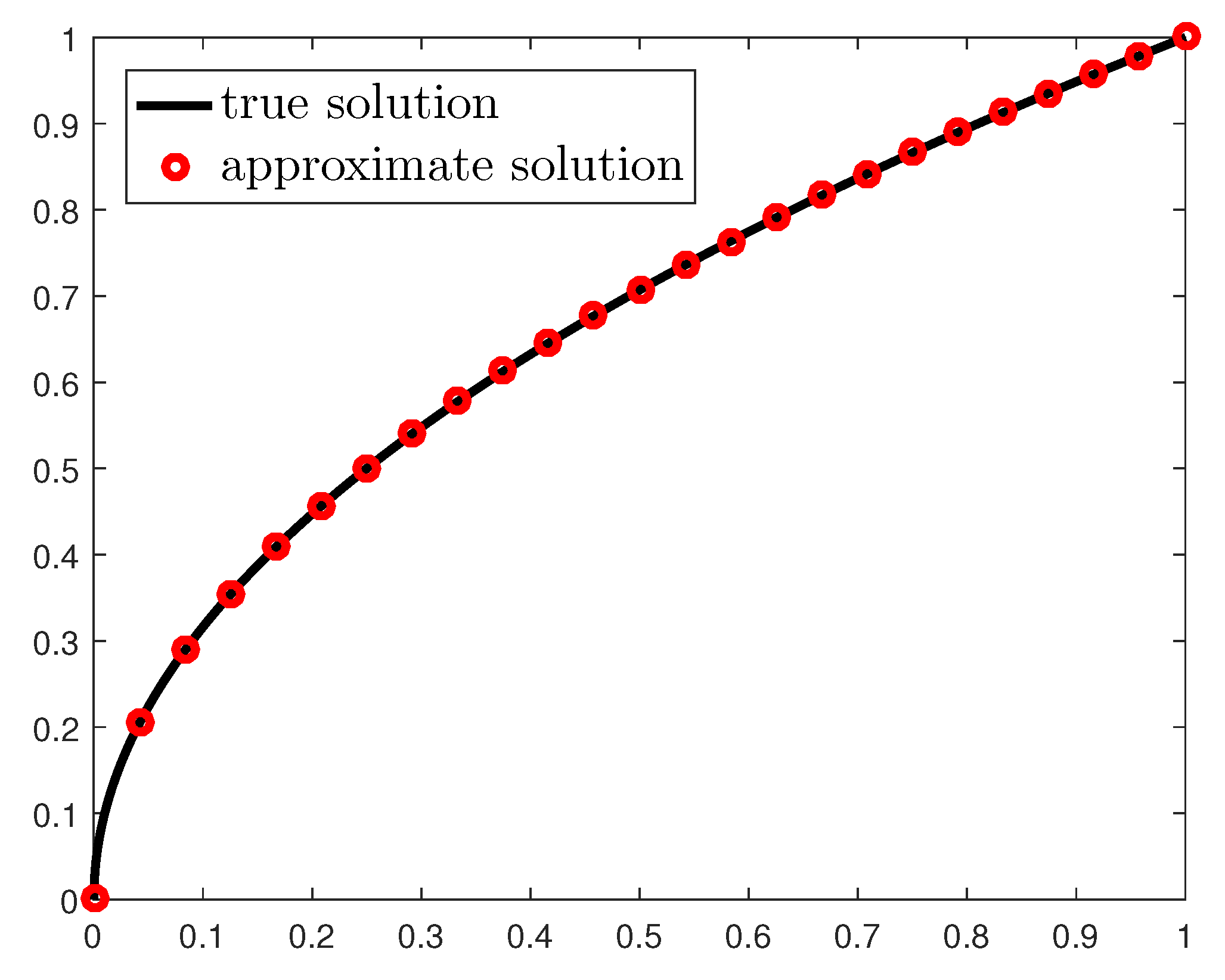
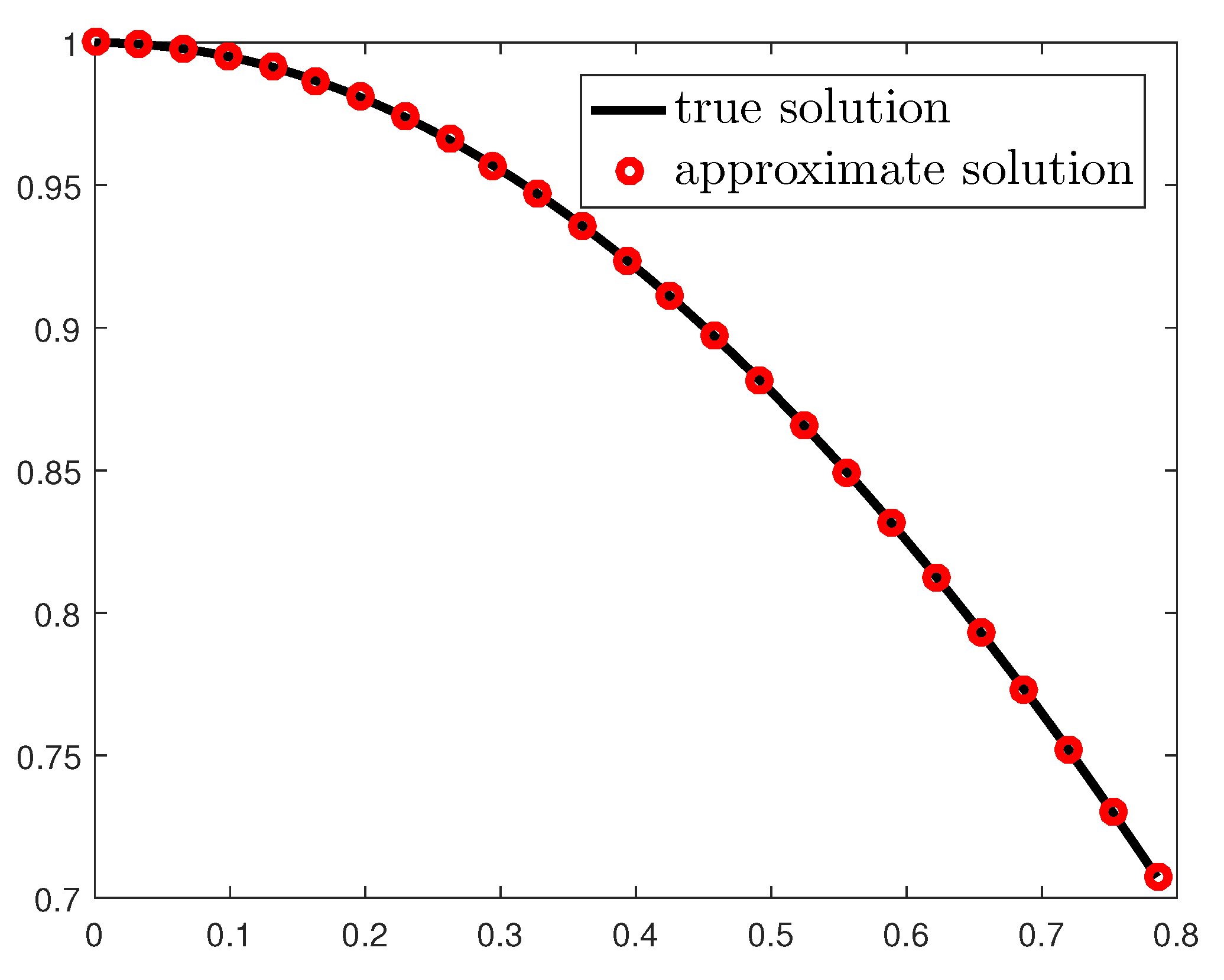
4. Numerical Experiments

In this section, we give numerical examples of nonlinear weakly singular integral equations, to show the applicability of the method proposed.

Example 1.

Consider the integral equation

$$\begin{array}{ccc}\hfill u\left(t\right)& =& {\displaystyle \frac{1}{12}}\underset{0}{\overset{t}{{\displaystyle \int }}}{u}^2\left(s\right){(t-s)}^{-1/2}ds+t^{1/2}\left(1-{\displaystyle \frac{1}{9}}t\right),t\in [0,1],\hfill \end{array}$$

with exact solution $u^{\ast }\left(t\right)=\sqrt{t}$.

We have $\alpha =1/2$, $a(t,s,u)={\displaystyle \frac{1}{12}}{u}^2$ and $f\left(t\right)=t^{1/2}\left(1-{\displaystyle \frac{1}{9}}t\right)$. Let us check that all our theoretical assumptions are met.

For the function f, $R_1=0,R_2=8/9$ and we choose $R=1$. Then $M={\displaystyle \frac{1}{12}}{\left({\displaystyle \frac{17}{9}}\right)}^2$$\approx 0.2973$ and for all $u\in [R_1-R,R_2+R],$

$$\begin{array}{ccc}\hfill {\displaystyle \frac{M{T}^{\alpha }}{\alpha }}& \approx & 0.5947\le R.\hfill \end{array}$$

We have ${\displaystyle \frac{\partial a}{\partial u}}={\displaystyle \frac{1}{6}}u$, so taking $L=max\left|{\displaystyle \frac{\partial a}{\partial u}}\right|$, over $u\in [R_1-R,R_2+R]$, $L\approx 0.3148$ and

$$\begin{array}{ccc}\hfill \gamma & \approx & 0.6296<1.\hfill \end{array}$$

Also, choosing $\tau =1$, we have

$$\begin{array}{ccc}\hfill {\displaystyle \frac{L\Gamma \left(\alpha \right)}{{\tau }^{\alpha }}}& \approx & 0.5580<1.\hfill \end{array}$$

Thus, all conditions of Theorem 5 are satisfied.

We apply the product trapezoidal rule for the values $m=12$ and $m=24$, with the corresponding nodes $t_k={\displaystyle \frac{1}{m}}k,k=\overline{0,m}$. In Table 1 we give the errors $e(u^{\ast },{\tilde{u}}_n)$, with initial approximation $u_0\left(t\right)=f\left(t\right)$. Figure 1 displays the graphs of the true solution $u^{\ast }\left(t\right)$ and of the approximate solution ${\tilde{u}}_n$, for $n=10$ iterations and $m=24$ nodes, for the values $t\in [0,1]$. As both the errors in Table 1 and the graphs in Figure 1 show, there is very good agreement between the true values and the approximate ones of the solution at the nodes $t_0,\dots ,t_m$.

Table 1. Errors $e(u^{\ast },{\tilde{u}}_n)$ for Example 1.

n	m
	12	24
1	1.084348 × 10${}^{-1}$	1.882162 × 10${}^{-2}$
5	2.799553 × 10${}^{-4}$	5.567188 × 10${}^{-6}$
10	6.813960 × 10${}^{-7}$	4.690204 × 10${}^{-9}$

Figure 1. Example 1, $n=10$, $m=24$.

Example 2.

Next, consider the equation

$$\begin{array}{ccc}\hfill u\left(t\right)& =& {\displaystyle \frac{1}{18}}\underset{0}{\overset{t}{{\displaystyle \int }}}\left({sin}^{2}s+u^2\left(s\right)\right){(t-s)}^{-2/3}ds+cost-{\displaystyle \frac{1}{6}}{t}^{1/3},t\in \left[0,\frac{\pi }{4}\right],\hfill \end{array}$$

whose exact solution is $u^{\ast }\left(t\right)=cost$.

Now $\alpha =1/3$, $a(t,s,u)=1/18\left({sin}^{2}s+u^2\right)$ and $f\left(t\right)=cost-t^{1/3}/6$. We check the applicability of the method, by verifying all the theoretical assumptions. Here, $R_1=f(\pi /4)\approx 0.5533,R_2=1$ and taking $R=1/2$, we have, for $u\in [R_1-R,R_2+R]$, $M=11/72\approx 0.1528$ and

$$\begin{array}{ccc}\hfill {\displaystyle \frac{M{T}^{\alpha }}{\alpha }}& \approx & 0.4229\le R.\hfill \end{array}$$

Again, taking $L=max\left|{\displaystyle \frac{\partial a}{\partial u}}\right|$, over $u\in [R_1-R,R_2+R]$, we get $L=1/6$ and

$$\begin{array}{ccc}\hfill \gamma & \approx & 0.4613<1.\hfill \end{array}$$

For $\tau =5$, we have

$$\begin{array}{ccc}\hfill {\displaystyle \frac{L\Gamma \left(\alpha \right)}{{\tau }^{\alpha }}}& \approx & 0.7227<1.\hfill \end{array}$$

So all conditions in Theorem 5 are verified.

Table 2 contains the errors $e(u^{\ast },{\tilde{u}}_n)$, with initial approximation $u_0\left(t\right)=f\left(t\right)$, for the values $m=12$ and $m=24$, with nodes $t_k={\displaystyle \frac{\pi }{4m}}k,k=\overline{0,m}$. Figure 2 shows the graphs of the true solution $u^{\ast }\left(t\right)$ and of the approximate solution ${\tilde{u}}_n$, for $n=10$ iterations and $m=24$ nodes, for $t\in [0,\pi /4]$.

Table 2. Errors $e(u^{\ast },{\tilde{u}}_n)$ for Example 2.

n	m
	12	24
1	1.002977 × 10${}^{-1}$	3.014020 × 10${}^{-2}$
5	2.315358 × 10${}^{-4}$	4.412851 × 10${}^{-5}$
10	9.363611 × 10${}^{-7}$	5.525447 × 10${}^{-9}$

Figure 2. Example 2, $n=10$, $m=24$.

As seen in the examples above, the proposed method produces approximations that are in very good agreement with the exact values of the solution, thus confirming the theoretical results and error estimates given in the previous section.

5. Conclusions

In this paper, we presented a numerical iterative method for approximating solutions of nonlinear Volterra integral equations of the second kind, with weakly singular kernels. We used Banach’s fixed point theorem to establish the existence and uniqueness of the solution and to find a sequence converging to it (Picard iteration). Then we employed the product trapezoidal rule to approximate each iteration at a given set of nodes in the domain. The present method is fairly simple to use, its convergence is based on a classical fixed point result. It is also quite efficient and inexpensive in (the cost of) implementation, most of the computations can be done only once, not at each iteration (see Remark 4). Thus, when only values of the solution at some points are needed (as is the case in many applications), this method is more practical and accessible than other classical methods.

Yet, the method converges quite fast, with order $O\left(q^n\right)$ with respect to the number of successive approximations and order $O\left(\frac{1}{m^2}\right)$ with respect to the number of nodes. As the examples show, it gives good approximations even with a relatively small number of iterations and of quadrature nodes.

In future works, other types of singularity of the kernel can be explored for Volterra or Fredholm integral equations. Also, more complicated kernels can be considered, such as kernels containing modified (or delayed) arguments, or other special types of kernels. Various other iteration techniques for fixed point successive approximations can be employed, such as Mann iteration, Krasnoselskii iteration, and others.

References

- Agarwal, R.P.; O’Regan, D. Singular Volterra integral equations. Appl. Math. Lett. 2000, 13, 115–120. [Google Scholar] [CrossRef]
- Gorenflo, R.; Vessella, S. Abel Integral Equations: Analysis and Applications, Lecture Notes in Mathematics (1461); Springer: Berlin, Germany, 1991. [Google Scholar]
- Wang, J.; Zhu, C.; Fečkan, M. Analysis of Abel-type nonlinear integral equations with weakly singular kernels. Bound. Value Probl. 2014, 2014, 20. [Google Scholar] [CrossRef]
- Becker, L.C. Properties of the resolvent of a linear Abel integral equation: Implications for a complementary fractional equation. Electron. J. Qual. Theory 2016, 64, 1–38. [Google Scholar] [CrossRef]
- Aghili, A.; Zeinali, H. Solution to Volterra singular integral equations and non homogenous time. Gen. Math. Notes 2013, 14, 6–20. [Google Scholar]
- Wu, G.C.; Baleanu, D. Variational iteration method for fractional calculus—A universal approach by Laplace transform. Adv. Differ. Equ. 2013, 2013, 18. [Google Scholar] [CrossRef]
- Andras, S. Weakly singular Volterra and Fredholm-Volterra integral equations. Stud. Univ. Babeş-Bolyai Math. 2003, 48, 147–155. [Google Scholar]
- Bertram, B.; Ruehr, O. Product integration for finite-part singular integral equations: Numerical asymptotics and convergence acceleration. J. Comput. Anal. Appl. 1992, 41, 163–173. [Google Scholar] [CrossRef]
- Brunner, H. The numerical solution of weakly singular Volterra integral equations by collocation on graded meshes. Math. Comput. 1985, 45, 417–437. [Google Scholar] [CrossRef]
- Diogo, T. Collocation and iterated collocation methods for a class of weakly singular Volterra integral equations. J. Comput. Appl. Math. 2009, 229, 363–372. [Google Scholar] [CrossRef]
- Assari, P. Solving weakly singular integral equations utilizing the meshless local discrete collocation technique. Alexandria Eng. J. 2018, 57, 2497–2507. [Google Scholar] [CrossRef]
- Rehman, S.; Pedas, A.; Vainikko, G. Fast solvers of weakly singular integral equations of the second kind. Math. Mod. Anal. 2018, 23, 639–664. [Google Scholar] [CrossRef]
- Kumar, S.; Kumar, A.; Kumar, D.; Singh, J.; Singh, A. Analytical solution of Abel integral equation arising in astrophysics via Laplace transform. J. Egypt. Math. Soc. 2015, 23, 102–107. [Google Scholar] [CrossRef]
- Mokharty, P.; Ghoreishi, F. Convergence analysis of the operational Tau method for Abel-type Volterra integral equations. Electron. Trans. Numer. Anal. 2014, 41, 289–305. [Google Scholar]
- Diogo, T.; Ford, N.J.; Lima, P.; Valtchev, S. Numerical methods for a Volterra integral equation with non-smooth solutions. J. Comput. Appl. Math. 2006, 189, 412–423. [Google Scholar] [CrossRef][Green Version]
- Ali, M.R.; Mousa, M.M.; Ma, W.-X. Solution of nonlinear Volterra integral equations with weakly singular kernel by using the HOBW method. Adv. Math. Phys. 2019. [Google Scholar] [CrossRef]
- Nadir, M.; Gagui, B. Quadratic numerical treatment for singular integral equations with logarithmic kernel. Int. J. Comput. Sci. Math. 2019, 10, 288–296. [Google Scholar]
- Alvandi, A.; Paripour, M. Reproducing kernel method for a class of weakly singular Fredholm integral eq uations. J. Taibah Univ. Sci. 2018, 12, 409–414. [Google Scholar] [CrossRef]
- Brunner, H.; Pedas, A.; Vainikko, G. The piecewise polynomial collocation method for nonlinear weakly singular Volterra equations. Math. Comput. 1999, 68, 1079–1095. [Google Scholar] [CrossRef]
- Darwish, M.A. On monotonic solutions of an integral equation of Abel type. Math. Bohem. 2008, 133, 407–420. [Google Scholar] [CrossRef]
- Sidorov, N.A.; Sidorov, D.N.; Krasnik, A.V. Solution of Volterra operator-integral equations in the nonregular case by the successive approximation method. Diff. Equ. 2010, 46, 882–891. [Google Scholar] [CrossRef]
- Sidorov, D.N.; Sidorov, N.A. Convex majorants method in the theory of nonlinear Volterra equations. Banach J. Math. Anal. 2012, 6, 1–10. [Google Scholar] [CrossRef]
- Noeiaghdam, S.; Dreglea, A.; He, J.; Avazzadeh, Z.; Suleman, M.; Fariborzi Araghi, M.A.; Sidorov, D.N.; Sidorov, N. Error Estimation of the Homotopy Perturbation Method to Solve Second Kind Volterra Integral Equations with Piecewise Smooth Kernels: Application of the CADNA Library. Symmetry 2020, 12, 1730. [Google Scholar] [CrossRef]
- Atkinson, K.E. An Introduction to Numerical Analysis, 2nd ed.; John Wiley & Sons: New York, NY, USA, 1989. [Google Scholar]
Publisher’s Note: MDPI stays neutral with regard to jurisdictional claims in published maps and institutional affiliations. |
© 2020 by the author. Licensee MDPI, Basel, Switzerland. This article is an open access article distributed under the terms and conditions of the Creative Commons Attribution (CC BY) license (http://creativecommons.org/licenses/by/4.0/).