Reading-Network in Developmental Dyslexia before and after Visual Training

Abstract

Electroencephalographic studies using graph-theoretic analysis have found aberrations in functional connectivity in dyslexics. How visual nonverbal training (VT) can change the functional connectivity of the reading network in developmental dyslexia is still unclear. We studied differences in the local and global topological properties of functional reading networks between controls and dyslexic children before and after VT. The minimum spanning tree method was used to construct the reading networks in multiple electroencephalogram (EEG) frequency bands. Compared to controls, pre-training dyslexics had a higher leaf fraction, tree hierarchy, kappa, and smaller diameter (θ—γ-frequency bands), and therefore, they had a less segregated neural network than controls. After training, the reading-network metrics of dyslexics became similar to controls. In β1 and γ-frequency bands, pre-training dyslexics exhibited a reduced degree and betweenness centrality of hubs in superior, middle, and inferior frontal areas in both brain hemispheres compared to the controls. Dyslexics relied on the left anterior temporal (β1, γ1) and dorsolateral prefrontal cortex (γ1), while in the right hemisphere, they relied on the occipitotemporal, parietal, (β1), motor (β2, γ1), and somatosensory cortices (γ1). After training, hubs appeared in both hemispheres at the middle occipital (β), parietal (β1), somatosensory (γ1), and dorsolateral prefrontal cortices (γ2), while in the left hemisphere, they appeared at the middle temporal, motor (β1), intermediate (γ2), and inferior frontal cortices (γ1, β2). Language-related brain regions were more active after visual training. They contribute to an understanding of lexical and sublexical representation. The same role has areas important for articulatory processes of reading.

1. Introduction

Reading is a multifaceted process that is supported by sublexical and lexical routes [1]. The sublexical route performs the transformation between graphemes and phonemes, which is used when reading unfamiliar words [2]. The lexical path is indispensable when reading incorrect words, favors the reading of regular words, and does not contribute to the reading of pseudo-words [2]. Skillful reading relies on the lexical route, which supports rapid recognition of the orthographic word form of familiar words [3]. The brain applies these two reading strategies along two different neuronal pathways: dorsal (occipitoparietal sublexical) and ventral (occipitotemporal lexical) routes [1]. When reading aloud, in contrast to silent comprehension tasks, children can rely on orthographic and phonological information and less on semantic information. Extracting words from memory is a major component in the production of language and articulation. The initial stages of learning to read are related to children with problems with orthographic code violations [2]. The children need to learn how letters or groups of letters (grapheme) are mapped to their respective phonemes. Training instructions begin with the explicit teaching of letter–sound or grapheme–phoneme rules. Then, children use these rules or associations to decode words they have heard but not seen before. This process of phonological decoding is the basis of reading comprehension [3]. After basic decoding skills acquirement, explicit teaching is being replaced by self-learning and begins to decode the words automatically [3]. Many children with dyslexia have poor phoneme awareness skills and problems with the process from the associative decoding network [4].

The phonological deficit, which implies a deficit in phonological awareness, followed by a visual deficit related to poor spelling due to poor coding of the position of letters (e.g., inversion of letters), and global noise, which suggests the overall inefficiency of processing due to noisy calculations [5], underlie developmental dyslexia. In them, it must be anticipated how correcting one component would change the reading efficiency of different types of words. The learning of reading has great interpersonal differences in vocabulary, phonology, and orthographic skills. Knowing the effectiveness of the reading network is useful for understanding reading difficulties.

Considering the human brain as a complex network of neurons and neuronal populations and the connections between them can lead to the emergence of complex patterns of connectivity between functionally diverse components. The “functional” relationships can be studied through statistical relationships between different functional components [6]. Brain networks are often studied in terms of functional segregation and integration. Functional segregation reflects the ability of the brain to specify locally information about the process, i.e., within a brain region or interconnected group of adjacent areas, while functional integration is the ability to combine information from different brain areas [7]. Functional analysis is a useful mathematical tool, which describes the brain networks as a set of nodes and their connections. Brain network integration and segregation can be characterized by graphical measures. The brain has been shown to exhibit properties of the small world [6]. Small world networks combine high local connectivity with high global integration. The small-world model was used in the study of the topological reorganization of functional brain networks during normal brain development [8] when the brain networks shift from a random topology to a more segregated small-world topology. Recent studies show that brain networks contain areas with tightly interconnected hubs, which process information in segregated modules, while the most important nodes, hubs, play a role in integrating information into the network [9].

The topology of functional brain networks plays an important role in understanding the human brain, normal functioning, pathology, and development. The brain networks of developmental dyslexia (DD) at rest have been well studied using an electroencephalogram [10]. Electroencephalogram (EEG) graph studies of the functional neural network of developmental dyslexia during the performance of tasks are missing.

Although developmental dyslexia has been thoroughly studied at the behavioral level, there is no consensus on its causes. Different behavioral studies of dyslexics have found various deficits in the sensitivity to a coherence motion perception [11], velocity discrimination [12,13], motion direction encoding [14,15], and contrast sensitivity to stimuli with low-/high-spatial frequency in external noise [16]. These deficits are selectively associated with low accuracy or with slow performance on reading sub-skills [17], problems with clearly seeing letters and their order, and the orienting and focusing of visual–spatial attention [16]. The deficits in the magnocellular pathway, established by the coherent motion perception, were associated with letter decoding disability. The magnocellular system is the visual input to the dorsal pathway that mediates motion perception and object localization [18], due to the projections to the visual motion-sensitive area and the posterior parietal cortex. For reading, the dorsal pathway has a major role in directing the visual attention and control of eye movements [15]. The effectiveness of intervention efforts has also been studied [19,20,21,22]. After visual magnocellular training, children with reading difficulties improved coherent motion detection, the saccadic eye movements, as well as reading accuracy and visual errors [23]. By detecting progressively faster movements in the coherent motion discrimination, the lexical decision and reading accuracy improved at the higher visual levels in the magnocellular system [20]. The phonological errors for dyslexic readers decreased after magnocellular intervention by figure–ground movement discrimination [23,24]. The reduction in phonological errors and visual timing deficits, the improvements in reading fluency, attention, phonological processing, and working memory are the result of improvement in the functioning levels of the dorsal stream. However, more research is needed to determine the neurophysiological causes of dyslexia. Some studies have focused on examining changes in the activity of specific brain regions [25], but recent research has shown that the causes of deficits may lie in a disrupted relationship between specific brain regions [9].

The question is whether the theory of functional analysis of developmental dyslexia can shed light on the neurophysiological reasons for the observed effectiveness of training with visual nonverbal tasks [17,19,23]. The hypothesis is that training with visual tasks in children with developmental dyslexia may lead to changes in their brain networks so that they are more similar to those in controls. The main questions were to determine (1) whether these changes would be mainly related to the dorsal (sublexical orthographic) pathway, which in turn may affect the functioning of the reading network and describe a deficit in language-related areas; and (2) whether the neural networks in children with DD can be reorganized after corrective visual nonverbal training.

The first goal of the study is to prove that network-level statistics is a useful tool to screen developmental dyslexia comparing controls and dyslexics. The second goal is to demonstrate that the visual nonverbal training can help reduce abnormality of the brain networks related to developmental dyslexia by network-level statistics between the pre- and post-training groups with dyslexia.

2. Materials and Methods

2.1. Research Design

A longitudinal study was conducted in the schools that involved repeated observations of the same children with developmental dyslexia over one school year. In this observational study with the exposure of visual intervention, the dyslexics are followed out over time to observe the outcome from the visual training and to evaluate the extent to which the visual tasks contribute to the alteration of this childhood disorder.

2.2. Children

Reliable electrophysiological data were obtained from forty-three children: 22 children with dyslexia (12 boys and 10 girls) and 21 normal children (11 boys and 10 girls). The age range for both groups was 8–9 years old. All children and their parents gave informed consent for an EEG following the Helsinki Declaration. The study was approved by the Ethics Committee of the Institute of Neurobiology, Bulgarian Academy of Sciences. The participants spoke Bulgarian as their first language. All children were right-handed and normal or corrected-to-normal vision. The handedness was assessed by a classification of hand preference. The participants had nonverbal intelligence scores of 98 or higher [26].

The children underwent a series of tests, including neuropsychological tests, a DDE-2 Battery (Battery for the Evaluation of Developmental dyslexia and Dysorthography) for the Evaluation of Developmental dyslexia and Dysorthography [27], reading and writing skills, psychometric tests for phonological awareness, Girolami-Boulinier’s “Different Oriented Marks” nonverbal perception test, and Raven’s Progressive Matrices test for nonverbal intelligence. In the group with dyslexia, children with reading difficulties were included, combined with below-norm performance in either speed or accuracy below one standard deviation from age-matched standardized control data in reading subtests of the DDE-2 battery (word list reading, pseudo-word list reading, choosing the correct meaning of a word, search for misspellings of words; writing of word/pseudo-word in dictation), as well as in the test battery “Reading abilities” (identifying the first sound in a heard word and omitting it in the word, fragmentation of the word in syllables and missed the last syllable, text reading, dictation of sentences filling in a missing compound word; Table S1). In the controls, age-matched children with the same socio-demographical background as the dyslexics were included, for whom there were no reported dyslexia or co-occurring language disorders confirmed by within-norm performance in speed and accuracy in reading.

2.3. Experimental Paradigm

Participants were exposed to visual stimuli (single words) presented on a laptop with a screen resolution of 1920 × 1080 pixels and a refresh rate of 60 Hz at a distance of 57 cm from the observer. The words remained on the computer screen for 800 ms and alternated in a pseudo-random sequence with the interstimulus interval (ISI: 1.5–2.5 s). The font was Microsoft Sans Serif (black letters on a white background). Each letter has an angular size of about 1 degree. The words were chosen according to their frequency of use, which was balanced according to their frequency characteristics—low and high frequency. The selected words were age-appropriate and covered parts of speech: nouns, adjectives, verbs, numbers, prepositions, adverbs, pronouns, and conjunctions.

The stimuli were presented in at least two blocks in daily EEG experimental sessions, each block containing 40 words. Participants were asked not to blink during stimulus presentation, only during the ISI to prevent artifacts in the EEG recordings during word reading. A behavioral parameter was assessed for each child: a voice reaction time (the time from the appearance of the word and the beginning of its reading). In addition, to examine whether visual perception training could affect the neural reading network of children with dyslexia, we recorded an EEG session during the reading of words one month after the three-month training with five visual nonverbal programs. Hence, irrespective of the word-reading task, the experimental group received an intensive procedure with training visual tasks, which were presented in an arbitrary order and divided twice a week in individual sessions lasting 45 min over a period of three months. This long-term period does not enable the children with developmental dyslexia to memorize information about the reading words in the task, which was performed before the training period.

Visual training consists of five visual programs that do not include any direct phonological input for children with developmental dyslexia. [11,13,15,17]. The training program, based on the direction discrimination of vertical coherent motion [11,28], stimulated the magnocellular function. Coherent vertical motion of white dots in randomly moving elements with a size of 0.1 deg was presented within a circle (diameter 20 deg) on a black screen at a viewing distance of 57 cm for 200 ms. The velocity of the moving dots was 4.4 deg/s. The coherent motion threshold was 50% of the randomly moving dots. The interstimulus interval was 1.5–2.5 s (ISI). The child was instructed to press a button with the left hand for the upward dot movements and to press a different button with a right hand when the dots in the stimulus move downwards.

The training program based on velocity discrimination [29] induced changes in the MT/V5 brain area. Two pair circular stimuli with radial moving white dots’ elements from the center to the periphery of optical flow (a diameter of 10 deg) appeared sequentially one after another on a screen. The first item in each pair of stimuli was always with a constant slow speed (4.5 deg/s). The second item in the pair of stimuli had a speed of the flow (5.0 deg/s) close to that of the first stimulus (4.5 deg/s) or with a higher (5.5 deg/s). The first item appeared for 300 ms, and after 500 ms, the second item in the stimulus pair appeared for 300 ms at a viewing distance of 57 cm. The ISI was 1.5–3.5 s. The instruction was to press a key with the right hand when the speed in the pairs was slow or another key with a left hand when the second stimulus in the pair had a higher speed than the constant speed of the first stimulus.

A low-contrast discrimination of low-spatial frequency sinusoidal gratings (2 cycles per degree of visual angle; cpd) and high-temporal frequencies (counter-phase flicker at 15 reversals/s), vertically flicking in external noise region (11 × 11 cm), maximally activated magnocellular cells [16,30]. The stimuli were presented in a center on a gray screen with a fixation cross. The contrast levels were 6% and 12% of the contrast threshold, which was defined in previously psychophysical experiments [31]. Gratings with different contrasts were presented in a pseudo-randomized sequence with an ISI of 1.5–3.5 s. The stimulus was subtended with a 2.7 × 2.7 deg visual angle at a viewing distance of 210 cm on a screen for 200 ms. Pressing the corresponding button with the left hand, the child discriminated low-contrast stimulus, while with the right hand, the child demonstrated sinusoidal grating with high contrast. High-contrast discrimination of high spatial frequency sinusoidal gratings (10 cpd), vertically flicking in the external noise region with contrast levels of 3% and 6% of a defined contrast threshold [31], were used to increase the parvocellular type activity. The other parameters of the task and the requirements for the child were the same as the previous task.

The visual–spatial attentional task with high peripheral processing demands was to search and track either the color change or color preservation of a square in a cue [32]. The cue was a black frame that appeared for 300 ms in either the left or right visual field on a white screen before the color square array (each with size 3 × 3 deg). A color square has appeared in the cue for 200 ms horizontally or vertically in an arranged color array of four squares. The cue remained on the screen during the presentation of the color array. The child had to compare the color of the square in the cue with the previous one that was presented in it on the screen at a viewing distance of 57 cm from the child. The adjacent squares in the array changed their colors in every presentation. The ISI was 1.5–2.5 s. The child pressed a key on a computer keyboard with a left hand when two consecutive colors in the cue were the same, and they pressed a key with the right hand when they were different. The number of correct answers and the reaction time were reported in the training programs with 40 trials in each condition and task. The thresholds of parameters and program designs were described in previous works [13,31].

2.4. EEG Recording and Signal Pre-Processing

The EEG is recorded with an internally developed 40-channel wireless EEG system using dry EEG sensors (each sensor is a matrix with 16 gold pins in the shape of a star; Brain Rhythm Inc., Taiwan). The reference sensors were placed on both the processi mastoidei and the ground sensor was placed on the forehead. The sensors were positioned on the head according to the international system 10-20: F3-4, C3-4, T7-8, P3-4, O1-2; Fz, Cz, Pz, and Oz; and additional positions according to system 10-10: AF3-4, F7-8, FT9-10, FC3-4, FC5-6, C1-2, C5-6, CP1-2, CP3-4, TP7-8, P7-8, PO3-04, and PO7-08. The skin impedance is controlled to be less than 5 kΩ. The EEG sampling rate is 250 Hz. Continuous EEG data are filtered by passing the band in the following frequency bands: δ = 1.5–4; θ = 4–8; α = 8–13; β1 = 13–20; β2 = 20–30; γ1 = 30–48; and γ2 = 52–70 Hz. The data were segmented into trials locked at the time of stimulus onset, each with a duration of 800 ms. Artifact-free EEG trials (≤±200 μV) with correct answers are included. We verified the signal-to-noise ratio (SNR) of the grand average stimuli evoked-related potentials (ERPs) [33]. The SNR criterion takes into account the noise around the ERP. SNRs were calculated using the formula SNR = A/(2 × SD_noise), where the amplitude A is the peak-to-peak voltage of the mean ERP, and SD_noise is the standard deviation of the noise (ε), which is obtained by subtracting the mean from each individual visual ERP. For a given single electrode, ε is just the collection of residuals, when the mean visual ERP is subtracted from each individual ERP, and SD_noise is the standard deviation over this collection. Cleaned EEGs were filtered (bandpass: 1–70 Hz; notch filter: 50 Hz). Only trials with correct responses and a high SNR were included in the analysis.

2.5. Functional Connectivity Analysis

The functional connectivity for all possible pairs of electrodes was determined using the phase lag index (PLI) [34]. This was done separately for each frequency band and trial. The PLI gives information about the phase synchronization of two signals, i.e., if one signal lags behind the other by measuring the asymmetry of the distribution of their instantaneous phase differences. The instantaneous phases can be calculated from the analytical signal based on the Hilbert transform. PLI = 0 indicates that two signals are not phase-locked (or that their phase difference is centered on 0 mod π). They are perfectly phase-locked with a phase difference different from 0 mod π and PLI = 1. The stronger this nonzero phase locking is, the larger the PLI will be. PLI does not depend on the amplitude of the signal and is less sensitive to volume conduction in the brain as well as spurious correlations because of common sources [34].

2.6. Minimum Spanning Tree

The calculated connectivities, using the PLI, between each pair of channels can construct an adjacency matrix, in which each row and each column represents a sensor, i.e., a graph that connects all its nodes (channels). Due to the methodological limitations such as sensitivity to alterations in connection strength (for weighted networks) or link density (for unweighted networks), which may occur concomitantly with alterations in network topology, the comparison of different brain networks can be problematic [7]. To avoid this problem, some authors have proposed the use of the minimum spanning tree (MST) to define an unbiased sub-graph of the original network [10]. It avoids methodological biases due to the mixing of information about topology with information about functional connectivity. The strengths of using the MST for brain network analysis are that it is a mathematically defined, unbiased sub-network that reflects the most fundamental network properties, while its characteristics are strongly related to conventional network metrics. This allows for unbiased comparison between networks of equal size in empirical studies. Changes in MST topology reflect changes in the underlying network topology. Even though the MST does not utilize all the connections in the network, it still provides a mathematically defined and unbiased sub-network with characteristics that can provide similar information about network topology as conventional graph measures.

A separate MST sub-graph was constructed from each of the PLI matrices, i.e., one for each non-rejected trial. The MST is a unique sub-graph that connects all the nodes of the graph without forming loops, such that the wiring cost (the weights) is minimized. The MST was constructed using Kruskal’s algorithm [35]. Since we were interested in the strongest connections, before using the algorithm, all the original weights (PLI) were converted to distances (1/PLI). The first step of the procedure is to order all the links in ascending order. After that, the link with the shortest distance (highest PLI) is added to the sub-network. Next, the link with the second shortest distance, which does not form any loops, is added, and this procedure is repeated until all the nodes are connected in an acyclic graph. All the links present in the MST are set to 1, while all the other connections are set to 0; i.e., the MST is a binary graph. The MST has a fixed density—M = N-1, where N is the number of nodes. There are two extreme MST topologies: (1) line-like topology, in which each node is connected to only two other nodes, with the exception of the two leaf nodes at either end of the line; and (2) star-like topology, in which, there is a single central node to which all the other nodes are directly connected. The MST captures most of the properties of a complex network in an unbiased sub-network, but due to the acyclicity, the resultant networks have lower density, which may lead to a loss of information about the original network [36]. The tree’s topology can be characterized by various measures. The global MST measures, similar to conventional graph measures, can provide information about network integration and segregation [7]. Four global MST measures were used in this study: diameter, leaf fraction, tree hierarchy, and kappa. The diameter in the MST is the shortest path along the minimum spanning tree. The shortest path between two nodes in the network is the path that involves the fewest number of links between them. It is a measure of the efficiency of a global network organization. Leaf fraction is the number of leaves (nodes with degree = 1) in the MST divided by the total number of nodes. The tree hierarchy is a metric that characterizes the balance of having high network integration without overloading information flow through the most important nodes in the network. There is an optimal topology with efficient organization when information overload of the central nodes is prevented. The tree hierarchy is defined as TH = L/2mBC_max, where m = N-1 links in the MST, N is the number of nodes, L is the number of leaves, BC is the fraction of all shortest paths that pass through a particular node, and BC_max is the maximal BC in the MST. TH has values between 0 and 1. On one extreme, if the tree has a line-like topology, i.e., L = 2, then if m approaches infinity, TH will approach 0. On the other end, if the tree is star-like, L = m and TH approaches 0.5. For topologies between these two extreme cases, TH will have higher values. The degree is the number of links for a given node. Kappa measures the broadness of the degree distribution in the network and has higher values for scale-free graphs and lower values for more random graphs. Kappa reflects the resilience of the network against attacks related to targeted hub removal, specifically a change in the degrees of the connected nodes. High kappa means the network is less vulnerable to random attacks, but it has higher vulnerability for targeted attacks. All these global MST measures were calculated separately for each non-rejected trial.

The nodal measures give information about the importance of individual nodes in the network. Two measures of nodal centrality were used in the subsequent analyses: degree and betweenness centrality (BC). The degree of a node is equal to the number of nodes to which it is connected. The betweenness centrality of a node is the fraction of all the shortest paths in the network that pass through that node. Nodes with a high degree or a high betweenness centrality play an important part in information processing in the network [37]. The networks are more integrated when they have a higher maximum degree or maximum betweenness centrality [37,38]. Hubs were defined as nodes with a degree or BC of at least 1 standard deviation above the mean. Links are the most important edges with at least 1 standard deviation above the mean.

2.7. Statistical Analysis

In EEG recording sessions, the voice response time of the dyslexic group before (pre-D) and after training (post-D) were compared for word reading as well as those of dyslexics and normal readers using the Kruskal–Wallis nonparametric test.

For each frequency band, between-group comparisons of the global MST measures were performed by a nonparametric permutation procedure with 1000 random shuffles [39]. Four graph indices (D, LF, TH, K) were compared between the groups in 28 (four indices x seven frequencies) independent permutation tests with correction for multiple comparisons. A Bonferroni correction to the significance level was applied separately for the tests of global indices (p = α/4 = 0.0125). The local measures (degree, BC) of the nodes were investigated to evaluate the local corporation of the brain regions, using separate nonparametric permutation cluster-based statistics (two indices × seven frequencies; [39]). The cluster-based nonparametric tests depend on a threshold, which is used to select the nodes that will subsequently be clustered. This analysis was performed for that maximum BC/or maximal degree that crosses the threshold selective criteria to define a hub (one standard deviation over the average group nodal BC/or degree). The localization procedure involved identifying clusters based on their cluster statistics. The critical value for the (max cluster) statistics was used to identify significant clusters while controlling the false alarm rate with correction for multiple comparisons, where multiple clusters exhibited a significant difference and quantified the effect by their ordered sequence. Their indices in the histograms are chosen so that their medians are sensitive to hemispheric differences. The selected threshold based on the data required Bonferroni correction of the significance level to control for multiple thresholds (p = α/2 = 0.025). Nonparametric statistical tests were performed in MATLAB. All the p-values that showed significant results are presented in bold text. The same selection criteria were performed separately for the edge BC, and the links crossing the threshold were presented in the figures.

3. Results

3.1. Behavior Results

Both dyslexic groups (pre-D: 1497.96 ± 30.5; post-D: 1266.16 ± 27.9 ms) showed 1.58 times slower vocal reaction time compared to the controls (873.5 ± 12.7 ms, p < 0.0001, χ² > 238.7). Post-D improved the voice response time 1.2 times compared to pre-D (p < 0.0001, χ² = 30.4).

3.2. Global Measures of MST

Statistically significant differences were found between global MST control measures and those of the pre-trained group with dyslexia. The smaller diameter and larger leaf fraction that dyslexic reading networks have in most bands are characteristic of a more integrated star-like topology (

Table 1. Nonparametric statistical comparison of global metrics (diameter, D; leaf fraction, LF; tree hierarchy, TH; kappa, K) of brain networks of control, pre-training and post-training dyslexic groups during word reading, for frequency bands: δ = 1.5–4; θ = 4–8; α = 8–13; β1 = 13–20; β2 = 20–30; γ1 = 30–48; γ2 = 52–70 Hz.

Metrics	Controls	Pre-Training Dys	Post-Training Dys	Con/Pre-Training Dys		Con/Post-Training Dys		Pre-/Post-Training Dys
	Mean ± s.e.	Mean ± s.e.	Mean ± s.e.	p	χ2	p	χ2	p	χ2
δ
D	0.263 ± 0.006	0.271 ± 0.003	0.276 ± 0.007	0.174	0.184	0.105	2.62	0.53	0.37
LF	0.618 ± 0.009	0.623 ± 0.005	0.608 ± 0.011	0.945	0.004	0.451	0.56	0.38	0.76
TH	0.413 ± 0.006	0.427 ± 0.003	0.419 ± 0.008	0.034	4.476	0.204	1.63	0.50	0.45
K	3.934 ± 0.133	4.004 ± 0.099	3.798 ± 0.145	0.968	0.001	0.379	0.72	0.23	1.32
θ
D	0.337 ± 0.004	0.311 ± 0.003	0.317 ± 0.004	<0.0001	21.22	0.0025	9.12	0.17	1.85
LF	0.531 ± 0.004	0.569 ± 0.004	0.555 ± 0.005	<0.0001	32.26	0.0014	10.14	0.067	3.34
TH	0.394 ± 0.004	0.409 ± 0.003	0.404 ± 0.004	0.004	8.13	0.036	4.36	0.60	0.27
K	3.019 ± 0.042	3.321 ± 0.041	3.195 ± 0.044	<0.0001	32.43	0.002	9.48	0.058	3.58
α
D	0.332 ± 0.003	0.316 ± 0.003	0.324 ± 0.004	0.001	10.35	0.088	2.89	0.27	1.16
LF	0.523 ± 0.004	0.552 ± 0.003	0.538 ± 0.004	<0.0001	26.34	0.035	4.42	0.011	6.44
TH	0.391 ± 0.003	0.402 ± 0.003	0.398 ± 0.003	0.026	4.93	0.275	1.18	0.333	0.93
K	2.943 ± 0.025	3.155 ± 0.031	3.041 ± 0.034	<0.0001	21.40	0.077	3.12	0.017	5.66
β1
D	0.333 ± 0.003	0.318 ± 0.002	0.333 ± 0.004	0.0002	14.13	0.762	0.09	0.0012	10.4
LF	0.507 ± 0.003	0.539 ± 0.003	0.519 ± 0.004	<0.0001	41.57	0.044	4.03	<0.0001	16.11
TH	0.374 ± 0.003	0.393 ± 0.003	0.387 ± 0.003	<0.0001	19.97	0.011	6.41	0.11	2.51
K	2.854 ± 0.021	3.056 ± 0.021	2.925 ± 0.023	<0.0001	46.11	0.024	5.08	<0.0001	15.84
β2
D	0.331 ± 0.003	0.315 ± 0.002	0.328 ± 0.003	0.0006	11.68	0.591	0.28	0.006	7.48
LF	0.506 ± 0.003	0.542 ± 0.003	0.517 ± 0.004	<0.0001	47.08	0.057	3.60	<0.0001	20.11
TH	0.377 ± 0.003	0.396 ± 0.003	0.385 ± 0.003	<0.0001	20.20	0.061	3.50	0.0238	5.01
K	2.829 ± 0.019	3.068 ± 0.024	2.898 ± 0.022	<0.0001	59.41	0.0238	5.10	<0.0001	24.22
γ1
D	0.329 ± 0.003	0.301 ± 0.003	0.315 ± 0.003	<0.0001	41.11	0.003	8.04	0.0025	9.07
LF	0.517 ± 0.004	0.566 ± 0.004	0.529 ± 0.004	<0.0001	70.91	0.085	2.95	<0.0001	39.51
TH	0.384 ± 0.003	0.409 ± 0.003	0.387 ± 0.003	<0.0001	29.44	0.635	0.22	<0.0001	22.65
K	2.866 ± 0.019	3.263 ± 0.033	2.958 ± 0.027	<0.0001	89.93	0.020	5.33	<0.0001	46.60
γ2
D	0.280 ± 0.002	0.262 ± 0.003	0.267 ± 0.003	<0.0001	24.28	0.001	10.62	0.188	1.72
LF	0.596 ± 0.003	0.636 ± 0.003	0.623 ± 0.004	<0.0001	60.79	<0.0001	29.80	0.055	3.66
TH	0.422 ± 0.003	0.441 ± 0.002	0.434 ± 0.003	<0.0001	18.32	0.009	6.72	0.207	1.59
K	3.427 ± 0.037	3.903 ± 0.048	3.708 ± 0.053	<0.0001	56.67	<0.0001	24.11	0.037	4.31

The significant level for global metrics after Bonferroni correction is p = 0.0125. Bold font shows statistically significant effects.

). On the other hand, the larger diameter and the smaller leaf fraction in the controls are indicative of a more segregated topology (Table 1). MST networks with smaller diameters tend to have a higher tree hierarchy and a higher kappa [8].

Significant differences in all global MST measures were found between the controls and the pre-trained group with dyslexia in the frequency bands θ, β, and γ for word reading. Compared to controls, pre-training dyslexics had a higher leaf fraction, tree hierarchy, kappa, and smaller diameter (p < 0.001, Table 1). The lower diameter (θ: χ² = 21.22, p < 0.0001) and the higher leaf fraction (θ: χ² = 32.26, p < 0.0001) of the pre-training group with dyslexia suggest a more integrated network compared to the controls. The pre-trained group with dyslexia also had a higher tree hierarchy compared to the controls (θ: p = 0.004; β1, β2, γ1, γ2: p < 0.0001; χ² > 19.97). The tree hierarchy reflects how optimal the MST configuration is, i.e., effective communication without overloading information flow through the hubs. The higher tree hierarchy and higher leaf fraction found in pre-training dyslexics point to a more loaded neural network than controls regarding information flow. After visual training, global MST measures revealed that in most frequency bands, the network topology of children with dyslexia has become more segregated and similar to the topology of controls. Exceptions were higher values of the leaf fraction in θ (p = 0.0014) and in γ2 (p = 0.0001), higher kappa in θ and γ2 (p < 0.002), and smaller diameter in θ, γ1, and γ2 (p = 0.0025, Table 1).

In α-frequency range, the leaf fraction and kappa decreased after training (p = 0.011; Table 1), indicating that the topology became more segregated than before training. In β1, β2, and γ1, the leaf fractions and kappa decreased after training (p < 0.0015; Table 1) compared to those before training. The tendency of the leaf fraction, kappa, and tree hierarchy to decrease after training (p < 0.0006; Table 1) is also present in the γ1 band. At γ2, their values for the post-training group with dyslexia remained significantly higher than those of the controls. In β1, β2, and γ1, the post-training group also showed a significant increase in diameter compared to pre-training group (p < 0.006; Table 1). The network of pre-training dyslexics could be more efficient due to the shorter diameter. However, pre-training the dyslexic network may result in an overload of information flow through the central hub nodes, where the communication largely depends on hub nodes (higher leaf fraction (LF)). They have a less optimal star-like topology of an effective organization (higher TH) and higher vulnerability for targeted attacks (higher kappa (K)).

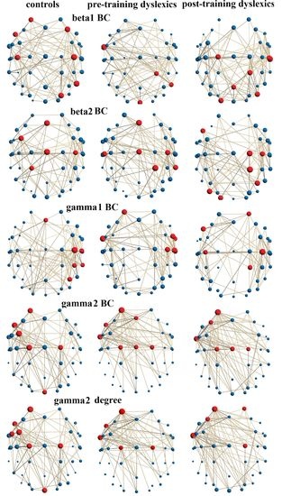
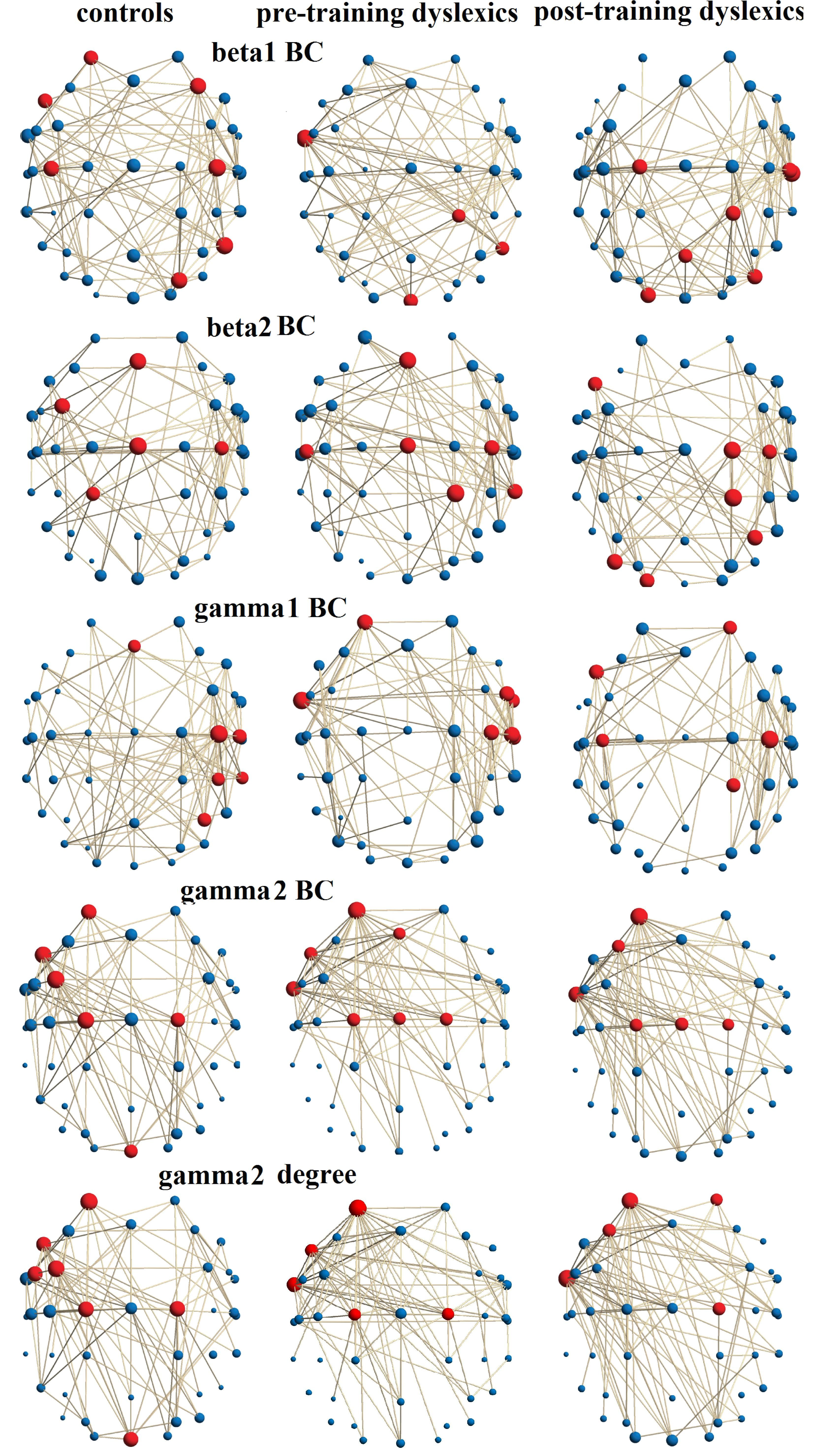
3.3. Distribution of Connectivity Hubs

When reading the words, the comparisons between the control group and the group with dyslexia in the β1-frequency range did not show significant differences in the hub distributions, based on the betweenness centrality (BC): between the controls and dyslexics before training (χ² = 0.91, p = 0. 338) and between controls and post-training dyslexics (χ² = 1.57, p = 0. 208; Figure 1A; Table S2). However, there was a statistically significant difference between hub distributions in the pre- and post-training group with dyslexia (χ² = 5.57; p = 0.018). The hubs for children with normal reading are located in the left superior frontal cortex (SFG; sensor AF3: BA9—dorsolateral prefrontal cortex [40]), right middle frontal gyrus (MFG; F4: BA8—intermediate frontal cortex), left inferior frontal gyrus (IFG; F7: BA45/47—Broca area, orbital frontal cortex), bilateral postcentral gyrus (PstCG; C3-4: BA123—primary somatosensory cortex), posterior part of right inferior temporal gyrus (ITG; P8: BA37—occipital temporal gyrus), and right superior occipital gyrus (SOG; PO4: BA19—associative visual cortex). Hubs in children with DD before training are in the anterior part of the left ITG (ATL; FT9: BA20—inferior temporal gyrus [40], BA38—temporal pole [41]), right ITG (P8: BA37 occipitotemporal gyrus), right superior parietal lobe (SPL; CP2: BA5- somatosensory association cortex [41]) and cuneus (Oz). After training in addition to hubs in the SPL (CP2), there were also hubs that were not in the pre-training reading network: in the right PstCG (C6: BA123—primary somatosensory cortex, BA40—supramarginal gyrus), left precentral gyrus (PreCG; C1: BA4, BA6—primary motor, premotor, and supplementary motor cortices), bilateral SPL (Pz: BA7), left middle temporal gyrus (MTG; T7: BA21) and bilateral middle occipital gyrus (MOG; PO8, O1: BA18—secondary visual cortex and inferior occipital gyrus [41]). Statistics also reveal a difference between the pre- and post-training groups that after training dyslexics had more hubs in the right hemisphere.

In contrast to the results for the β1-frequency range, in β2, there was a significant difference in the hub distribution determined by the betweenness centrality (BC) between the controls and the group with dyslexia after training (χ² = 4.71, p = 0.025; Figure 1B, 1st, 3rd graphs; Table S2). For the control group, the hubs were located in the bilateral superior frontal cortex (SFC; Fz: BA6—premotor cortex), left MFG (FC3: BA6—premotor and supplementary motor cortices), bilateral PreCG (Cz: BA4), right PstCG (C4) and left SPL (CP1). For the post-training group, the hubs were not only in the right PstCG (C4), right SPL (CP2), but additionally in the left IFG (F7), right PreCG (C2), right inferior parietal lobe IPL (P4: BA39—angular gyrus), and left MOG (PO7, O1; Figure 1B, 2nd). The differences in the networks of the two groups are due to there being more hubs in the anterior part of the left hemisphere of the controls, while dyslexics after training had more in the posterior part of the right hemisphere. For the pre-training group with dyslexia, the hubs were located in the SFC (Fz), PstCG (C5), bilateral PreCG (Cz: BA4), right PstCG (C4), right SPL (CP2), and right MTG (TP8: BA21; Figure 1B, 2nd). The comparison of the hub distributions between the controls and the dyslexics before training did not show a statistical difference (β2: χ² = 0.49, p = 0.485). There was no statistical difference in the hub distributions between the pre- and post-training group with dyslexia (χ² = 3.15, p = 0.075).

Between-group hubs comparisons (BC) also revealed a statistically significant difference between controls and the pre-trained group with dyslexia in the γ1-frequency range (χ² = 7.37, p = 0.006; Table S2), where the children with dyslexia were showing more hubs in the left hemisphere compared to the controls. The main hubs in the controls were located in the bilateral SFG (Fz), right PstCG (C4, C6), right IPL (CP4: BA40—supramarginal gyrus; P4: BA39—angular gyrus), MTG (TP8; Figure 1C, 1st). For the untrained group with dyslexia, the hubs were distributed in the left SFG (AF3), bilateral ATL (FT9-10), and in the right hemisphere at the inferior frontal gyrus (IFG; FC6: BA44/45—opercular and triangular parts of Broca’s area), PstCG (C4, C6), and MTG (T8; Figure 1C, 2nd graph). After training, the hubs were located in the right SFG (AF4), left IFG (F7), bilateral PstCG (C3-4), and right SPL (CP2, Figure 1C, 3rd). The statistics did not show significant differences between controls and the post-training group with dyslexia (χ² = 1.72, p = 0.188). There was no significant difference between the dyslexics before and after training (χ² = 1.29, p = 0.25).

At γ2 frequencies, comparisons of hub distributions between groups (based on BC) revealed significant differences between controls and the pre-training dyslexics (χ² = 13.62, p = 0.0002; Table S2), as the controls had more hubs in the left hemisphere. Their main hubs were the left SFG (AF3), left MFG (FC3), left IFG (F7), bilateral PreCG (C1–2), and cuneus (Oz). The main hubs of the pre-training group were at the bilateral SFG (Fz, AF3), left IFG (F7), left ATL (FT9), and bilateral PreCG (Cz, C1-2), while after training, they were at the SFG (AF3), MFG (F3), ATL (FT9), and PreCG (Cz, C1-2). There were no significant differences in their distributions (pre-D vs. Post-D; χ² = 1.84, p = 0.173), as well as between controls and dyslexics after training (χ² = 3.79, p = 0.051). The hub distributions differed between controls and the pre-training group with dyslexia in the γ2 reading network (χ² = 7.37, p = 0.006; Figure 1E), as pre-training dyslexic hub distributions were displaced more anteriorly than the control group. In controls, hubs were located in the left SFG (AF3), MFG (FC3), IFG (F7, FC5), bilateral PreCG (C1-2), and cuneus (Oz; Figure 1E, 1st), while before training in the group with dyslexia, the hubs were in the left hemisphere in SFG (AF3), IFG (F7), ATL (FT9), and bilateral PreCG (C1-2; Figure 1E, 2nd). For the post-training group, the hubs were the bilateral SFG (AF3-4), left MFG (F3), left ATL (FT9), and right PreCG (C2). The difference between the group with dyslexia before and after training was significant (χ² = 8.54, p = 0.003), due to more hubs in the right hemisphere after training. The difference between the controls and the post-training group with dyslexia was not significant (χ² = 1.40, p = 0.236).

4. Discussion

4.1. Altered Global Topology in Developmental Dyslexia

This MST-based graphical analytical approach examines the topology of functional networks in the brain, which were derived from EEG data for both controls and children with developmental dyslexia when reading aloud single words. Before training, the global topological organization of the children with dyslexia is different from that of the controls. After their training, their global topological measures become more similar to that of controls. The diameter of the MST is the largest for regular networks and decreases in random networks. The diameter and leaf fraction have extreme values for scale-free networks, i.e., the diameter is the lowest, and the leaf fraction is the highest in a scale-free network [7]. The smaller diameter and higher leaf fraction for most frequency bands, in pre-training children with dyslexia, is indicative of a more integrated star-like topology than controls that showed a more decentralized network. Compared to typically developing children, the dyslexics exhibited a different global brain topology when reading words.

An efficient network would be one that optimally balances between local processing and global integration. The more integrated network of pre-training dyslexics could reflect a less optimal global organization with an overloading information flow through the central connectivity hubs (brain areas). A recent MRI study of the structure of the brain networks of Chinese children with dyslexia found that they, compared to controls, had altered topological organization in rest with increased local and reduced global efficiency [42]. The higher diameter and the lower leaf fraction, tree hierarchy, and kappa found in the controls, compared to the pre-training dyslexics, could reflect a more mature brain.

After training, the changes in the MST measures of children with dyslexia were similar to the changes observed in the process of brain maturation [8]. The increase of topological segregation after training decreases the load on the important brain regions, leading to a more balanced brain network, analogous to the processes, observed in the brain development of children [43]. The change in network topology after training could be the result of a compensatory mechanism.

The between-group differences in MST measures were mostly frequency-independent. They had a similar profile in most of the bands, suggesting that similar network constraints occur in different neural circuits. Significant correlations have been found between network indices and phonological decoding ability in α and β2 EEG bands [44]. The idea that dyslexics may exhibit differences in brain connectivity would be consistent with the evidence and theoretical models suggesting deficits in general sensory functions and attention that are associated with higher frequency EEG activity (beta and gamma).

Our results revealed that, compared to typically developing children, the dyslexics exhibit a different topological organization of their brain networks and that with training, these networks reorganize and become more segregated. These changes after training are similar to the changes observed in brain maturation, in which the smaller diameter and the higher leaf fraction that children have, compared to adults, indicate that the topology of the functional brain networks becomes less centralized with development [8]. The lower tree hierarchy and kappa after training also indicate a better-balanced network with a lower risk of an overload of its most important regions. Changes in the segregation of brain functional systems during brain development are related to improving the brain network organization, which is characterized by increasing segregation between the functional systems of the brain regions and increasing the specialization of their functions. The reduced segregation of task-related brain systems of dyslexics before training that accompanies new performance tasks subside with continued practice, leading to the automation of some tasks.

Increasing segregation in the brain systems of typical children is associated with a high cognitive ability as good long-term episodic memory [45]. The relationship between systemic segregation and cognitive ability sustains independently of age throughout life. Brain networks, which have segregated systems, are flexible to certain types of interference. A brain disorder, especially caused in crucial hub locations, is associated with increased functional connectivity between the systems or reduced segregation [46]. Dyslexics who have undergone cognitive remedy training provide additional support necessary for systematic segregation to promote cognition [47,48]. Post-trained dyslexics with a higher level of segregation than before training may beneficially change cognition with training.

4.2. Distribution of the Connectivity Hubs

The basic reading neural network in normally reading children at β1 frequencies includes frontotemporoparietal chains primarily in the left hemisphere of the brain [49]. During word reading, early visual processing occurs in the right inferior occipitotemporal cortex and the superior occipital gyrus [50], which is the starting point for the two main hubs transmitting information forward in the reading network [51]. After the right occipitotemporal area, the reading network includes the bilateral postcentral gyri (motor cortex, primary somatosensory cortex), left inferior frontal cortex (pars triangularis), and dorsolateral prefrontal cortex [49]. These brain regions allow for the understanding of lexical and sublexical phonological representation and play a role in articulatory processes important for reading [52,53,54,55,56,57]. Functional abnormalities in the β1 frequencies, observed in pre-training children with developmental dyslexia, demonstrate the absence of hubs in the superior, middle, and inferior frontal areas in both hemispheres. Hubs predominate in the anterior temporal lobe in the left hemisphere and in the right hemisphere at the superior parietal and inferior occipitotemporal areas (including fusiform area). After training, hubs in the group with dyslexia appear in the left hemisphere at the middle temporal gyrus, bilateral superior parietal and bilateral middle occipital gyri, right somatosensory and supramarginal cortices, left primary motor, premotor, and supplementary motor cortices. The β2-reading network of normal children consists of the left superior parietal gyrus, right postcentral, bilateral motor and premotor areas, and right primary somatosensory cortex. These brain regions play a role in articulatory processes important for reading [52]. The functional abnormalities observed in developmental dyslexia demonstrate deactivation of the left frontal areas in the inferior frontal gyrus, which is accompanied by overactivation in the right hemisphere at the primary motor cortex and middle temporal gyrus [55,56]. For the post-training group with dyslexia, hubs with BCmax are present not only in the right somatosensory association cortex but also in the left inferior frontal gyrus, the right angular, and the left middle occipital gyri.

In normal children, the γ1-reading network consists of the bilateral premotor cortices and, in the right hemisphere, the primary somatosensory cortex, supramarginal, angular, and middle temporal gyri. Meanwhile, in the post-training children with dyslexia, the γ1-reading network includes the left inferior frontal, right dorsolateral prefrontal, bilateral primary somatosensory cortices, and right somatosensory association cortex. The pre-training group with DD is characterized by deactivation of the left inferior frontal cortex in the γ1-reading network, and by the appearance of hubs in the right inferior frontal cortex, primary somatosensory cortex, supramarginal, middle temporal, and bilateral anterior temporal gyri, and left dorsolateral prefrontal cortex.

During word reading, early visual processing in the γ2 neural network occurs in the bilateral occipital cortex, which is the starting point for major hubs transmitting information forward in the left hemispheric reading network to the premotor and supplementary motor cortices, bihemispheric primary motor, inferior frontal (pars triangularis), and dorsolateral prefrontal cortices [49]. In the group after training, hubs appeared also in the left intermediate frontal cortex as well as in both hemispheres in the dorsolateral prefrontal cortices. Functional abnormalities in the γ2 frequency band, observed in pre-training dyslexics, demonstrated the absence of hubs in the left hemisphere of the middle frontal areas, premotor and supplementary motor cortices, as well as in both hemispheres of the visual brain areas, but a hub was observed in the left inferior frontal cortex.

The neuronal reading system includes frontal, temporoparietal, temporal cortical areas, and other brain areas, and it also includes functions outside the reading system [1], particularly in areas related to visual and semantic processes. This learning process has profound functional effects on brain development [58]. Children, who spend more time reading, have a stronger functional connection between the fusiform gyrus, the area related to word processing in reading, and the visual and cognitive areas [59]. Reading as a complex task involves a number of different areas and functions of the brain in which visual, phonological, orthographic, and semantic systems play an important role in this process. These systems are represented by the occipital cortex, supramarginal, fusiform gyri, and anterior temporal cortex. Areas related to reading such as the frontal opercular and temporal cortices are key regions for the reading process. Beyond the reading-related brain systems, the auditory cortex is also associated with reading achievement [60], as well as the role attributed to phonological awareness in the acquisition of reading. The presentation of aloud reading is closely related to the activity of the left motor and somatosensory cortices [61]. Visual areas also contribute to reading [1], as reading words requires visual word processing. There are also language-related areas in reading-related networks, especially semantic areas such as inferior frontal, inferior temporal, and superior temporal cortices [62].

Reading networks include both hemispheres. Many previous studies have found that reading is left lateralized, and it is composed of phonological and orthographic systems, including the frontal area of Broca and the left fusiform area, respectively [63]. The left fusiform gyrus plays an important role in reading whole words [64]. However, the strict left lateralization of reading has been altered later by many studies on the additional involvement of the right hemisphere [65]. The two hemispheres work together to carry out the reading process in different frequency ranges of the acoustic speech envelope [66]. In addition, the contribution of the right hemisphere to lexical processes shapes individual differences in reading ability [67]. The contribution of the right hemisphere, including the prefrontal and posterior temporal areas to language comprehension, has also been linked to reading [68]. Reading involves many cognitive processes with more or less specific neural substrates. The two hemispheres contribute to reading but in very specific ways.

Most functional connections associated with reading occur in the parietal and frontal cortices in both hemispheres of the brain, and they are responsible for higher-order cognitive functions. The least reading-related functional connections dominate in the right hemisphere, especially at the γ1 network, and they are more expressed in the pre-D group (BC). The density of connections inside reading networks is higher than that outside reading networks [1]. In general, connections between brain areas could carry more information about behavioral characteristics. Interconnection between the language areas in the left hemisphere and those for attention in the right hemisphere is underlying both the lexical and the sublexical reading.

The left lateralization of the frontal areas in post-training dyslexics compared to those before training (β2) suggests functional impairment of a major language center such as the left frontal cortex. Some brain areas such as the frontal, occipital, middle, and superior temporal cortices, as well as the parietal/occipital cortex near the angular gyrus, specialize mainly in the left hemisphere during the acquisition of reading skills [69].

The simultaneous appearance of hubs in the left inferior frontal lobe and the visual word-form area, which is present in the controls (β1, γ2) and the post-training dyslexics (β2), are not observed in pre-training children with dyslexia (β1, β2). It might be associated with reading development [70]. The absence of hubs adjacent to the Heschl’s sulcus in pre-training children with DD (β1) has been found to be an early sign of dyslexia in other studies [42].

The presence of hubs in children with developmental dyslexia after training in the dorsal visual network, including the inferior parietal, middle temporal, visual associative cortex, and the dorsal superior frontal cortex, suggests that the training in the visual modality affects the distribution of nodes in children with developmental dyslexia. Therefore, the research confirms the hypothesis that the disturbed phonological decoding in dyslexia, occurring in the processing of visual and auditory stimuli, is influenced positively after training in the visual modality [71,72]. The heteromodal, as well as some modality-specific areas, are involved in the reading processing.

5. Conclusions

In general, these observations highlight the heterogeneity of hub processing within functionally specialized brain systems and reveal how key roles of individual hubs may be disrupted by changes in brain system segregation. Effective task execution requires greater interactivity between distribution hubs in multiple brain systems, which is achieved by segregation of the task-related components of the network organization. In the brains of typical children, the diverse connectivity of interconnecting hubs engaged in a wide variety of tasks probably mediates a wide repertoire of functions and allows them to flexibly integrate and transfer information between individual functional systems. Reading-related and modality-related hub distinctions in dyslexic networks are reduced in brain networks that show less systematic segregation.

Some methodological limitations of the MST study are related to some measures sensitive to the network size, which may affect the relative importance of the nodes in the operation of the network. The main limitation of the segregation analysis is related to the choice of a threshold for the distribution of hubs, which emphasizes the regions with BC at least one standard deviation above the mean and avoids the choice of these nodes with lower intensity links.

References

1. Dehaene, S.; Cohen, L.; Morais, J.; Kolinsky, R. Illiterate to literate: Behavioural and cerebral changes induced by reading acquisition. Nat. Rev. Neurosci. 2015, 16, 234–244. [Google Scholar] [CrossRef] [PubMed]
2. Castles, A.; Rastle, K.; Nation, K. Ending the Reading Wars: Reading Acquisition from Novice to Expert. Psychol. Sci. Public Interes. 2018, 19, 5–51. [Google Scholar] [CrossRef] [PubMed]
3. Share, D.L. Phonological recoding and self-teaching: Sine qua non of reading acquisition. Cognition 1995, 55, 151–218. [Google Scholar] [CrossRef]
4. Landerl, K.; Ramus, F.; Moll, K.; Lyytinen, H.; Leppänen, P.H.T.; Lohvansuu, K.; O’Donovan, M.; Williams, J.; Bartling, J.; Bruder, J.; et al. Predictors of developmental dyslexia in European orthographies with varying complexity. J. Child Psychol. Psychiatry 2012, 54, 686–694. [Google Scholar] [CrossRef] [PubMed]
5. Hancock, R.; Pugh, K.R.; Hoeft, F. Neural Noise Hypothesis of Developmental Dyslexia. Trends Cogn. Sci. 2017, 21, 434–448. [Google Scholar] [CrossRef] [PubMed] [Green Version]
6. Bassett, D.S.; Bullmore, E. Small-World Brain Networks. Neuroscience 2006, 12, 512–523. [Google Scholar] [CrossRef] [PubMed]
7. Tewarie, P.; Van Dellen, E.; Hillebrand, A.; Stam, C.J. The minimum spanning tree: An unbiased method for brain network analysis. NeuroImage 2015, 104, 177–188. [Google Scholar] [CrossRef] [PubMed]
8. He, W.; Sowman, P.F.; Brock, J.; Etchell, A.C.; Stam, C.J.; Hillebrand, A. Increased segregation of functional networks in developing brains. NeuroImage 2019, 200, 607–620. [Google Scholar] [CrossRef]
9. Rubinov, M.; Sporns, O. Complex network measures of brain connectivity: Uses and interpretations. Neuroimage 2010, 52, 1059–1069. [Google Scholar] [CrossRef]
10. González, G.F.; Van Der Molen, M.; Žarić, G.; Bonte, M.; Tijms, J.; Blomert, L.; Stam, C.J.; Van der Molen, M.W. Graph analysis of EEG resting state functional networks in dyslexic readers. Clin. Neurophysiol. 2016, 127, 3165–3175. [Google Scholar]
11. Boets, B.; Vandermosten, M.; Cornelissen, P.; Wouters, J.; Ghesquière, P. Coherent Motion Sensitivity and Reading Development in the Transition from Prereading to Reading Stage. Child Dev. 2011, 82, 854–869. [Google Scholar] [CrossRef]
12. Demb, J.B.; Boynton, G.M.; Best, M.; Heeger, D.J. Psychophysical evidence for a magnocellular pathway deficit in dyslexia. Vis. Res. 1998, 38(11), 1555–1559. [Google Scholar] [CrossRef] [Green Version]
13. Lalova, J.; Dushanova, J.; Kalonkina, A.; Tsokov, S. Application of specialised psychometric tests and training practices in children with developmental dyslexia. Psychol. Res. 2019, 22, 271–283. [Google Scholar]
14. Cornelissen, P.L.; Hansen, P.C.; Hutton, J.L.; Evangelinou, V.; Stein, J.F. Magnocellular visual function and children’s single word reading. Vision Res. 1998, 38, 471–482. [Google Scholar] [CrossRef]
15. Stein, J.F. Dyslexia: The Role of Vision and Visual Attention. Curr. Dev. Disord. Rep. 2014, 1, 267–280. [Google Scholar] [CrossRef] [Green Version]
16. Sperling, A.J.; Lu, Z.-L.; Manis, F.R.; Seidenberg, M.S. Deficits in perceptual noise exclusion in developmental dyslexia. Nat. Neurosci. 2005, 8, 862–863. [Google Scholar] [CrossRef]
17. Wilmer, J.B.; Richardson, A.; Chen, Y.; Stein, J.F. Two Visual Motion Processing Deficits in Developmental Dyslexia Associated with Different Reading Skills Deficits. J. Cogn. Neurosci. 2004, 16, 528–540. [Google Scholar] [CrossRef]
18. Goodale, M.A.; Westwood, D.A. An evolving view of duplex vision: Separate but interacting cortical pathways for perception and action. Curr. Opin. Neurobiol. 2004, 14, 203–211. [Google Scholar] [CrossRef]
19. Lawton, T. Improving magnocellular function in the dorsal stream remediates reading deficits. Optom. Vis. Dev. 2011, 42, 142–154. [Google Scholar]
20. Chouake, T.; Levy, T.; Javitt, D.C.; Lavidor, M. Magnocellular training improves visual word recognition. Front. Hum. Neurosci. 2012, 6, 14. [Google Scholar] [CrossRef] [Green Version]
21. Qian, Y.; Bi, H.-Y. The effect of magnocellular-based visual-motor intervention on Chinese children with developmental dyslexia. Front. Psychol. 2015, 6. [Google Scholar] [CrossRef] [Green Version]
22. Lawton, T.; Shelley-Tremblay, J. Training on Movement Figure-Ground Discrimination Remediates Low-Level Visual Timing Deficits in the Dorsal Stream, Improving High-Level Cognitive Functioning, Including Attention, Reading Fluency, and Working Memory. Front. Hum. Neurosci. 2017, 11, 236. [Google Scholar] [CrossRef] [Green Version]
23. Ebrahimi, L.; Pouretemad, H.; Khatibi, A.; Stein, J. Magnocellular Based Visual Motion Training Improves Reading in Persian. Sci. Rep. 2019, 9, 1–10. [Google Scholar] [CrossRef]
24. Lawton, T. Improving Dorsal Stream Function in Dyslexics by Training Figure/Ground Motion Discrimination Improves Attention, Reading Fluency, and Working Memory. Front. Hum. Neurosci. 2016, 10, 397. [Google Scholar] [CrossRef] [PubMed] [Green Version]
25. Habib, M. The neurological basis of developmental dyslexia: An overview and working hypothesis. Brain 2000, 123, 2373–2399. [Google Scholar] [CrossRef]
26. Raven, J.; Raven, J.C.; Court, J.H. Manual for Raven’s Progressive Matrices and Vocabulary Scales; Section 2: The coloured progressive, matrices; Oxford Psychologists Press: Oxford, UK; The Psychological Corporation: San Antonio, TX, USA, 1998. [Google Scholar]
27. Sartori, G.; Remo, J.; Tressoldi, P.E. Updated and revised edition for the evaluation of dyslexia. In DDE-2, Battery for the Developmental Dyslexia and Evolutionary Disorders-2, 1995; Giunti O.S.: Florence, Italy, 2007. [Google Scholar]
28. Benassi, M.; Simonelli, L.; Giovagnoli, S.; Bolzani, R. Coherence motion perception in developmental dyslexia: A meta-analysis of behavioral studies. Dyslexia 2010, 16, 341–357. [Google Scholar] [CrossRef]
29. Joshi, M.R.; Falkenberg, H.K. Development of radial optic flow pattern sensitivity at different speeds. Vis. Res. 2015, 110, 68–75. [Google Scholar] [CrossRef] [Green Version]
30. Pammer, K.; Wheatley, C. Isolating the M(y)-cell response in dyslexia using the spatial frequency doubling illusion. Vis. Res. 2001, 41, 2139–2147. [Google Scholar] [CrossRef] [Green Version]
31. Lalova, J.; Dushanova, J.; Kalonkina, A.; Tsokov, S.; Hristov, I.; Totev, T.; Stefanova, M. Vision and visual attention of children with developmental dyslexia. Psychol. Res. 2018, 21, 247–261. [Google Scholar]
32. Ross-Sheehy, S.; Oakes, L.M.; Luck, S.J. Exogenous attention influences visual short-term memory in infants. Dev. Sci. 2011, 14, 490–501. [Google Scholar] [CrossRef] [Green Version]
33. Dushanova, J.; Christov, M. Auditory event-related brain potentials for an early discrimination between normal and pathological brain aging. Neural Regen. Res. 2013, 8, 1390–1399. [Google Scholar]
34. Stam, C.J.; Nolte, G.; Daffertshofer, A. Phase lag index: Assessment of functional connectivity from multi channel EEG and MEG with diminished bias from common sources. Hum. Brain Mapp. 2007, 28, 1178–1193. [Google Scholar] [CrossRef]
35. Kruskal, J.B. On the shortest spanning subtree of a graph and the traveling salesman problem. Proc. Am. Math. Soc. 1956, 7, 48. [Google Scholar] [CrossRef]
36. Smith, K.; Abásolo, D.; Escudero, J. Accounting for the complex hierarchical topology of EEG phase-based functional connectivity in network binarisation. PLoS ONE 2017, 12, e0186164. [Google Scholar] [CrossRef] [PubMed]
37. Bullmore, E.T.; Sporns, O. Complex brain networks: Graph theoretical analysis of structural and functional systems. Nat. Rev. Neurosci. 2009, 10, 186–198. [Google Scholar] [CrossRef]
38. Stam, C.; Tewarie, P.; Van Dellen, E.; Van Straaten, E.; Hillebrand, A.; Van Mieghem, P. The trees and the forest: Characterization of complex brain networks with minimum spanning trees. Int. J. Psychophysiol. 2014, 92, 129–138. [Google Scholar] [CrossRef] [Green Version]
39. Maris, E.; Oostenveld, R. Nonparametric statistical testing of EEG- and MEG-data. J. Neurosci. Methods 2007, 164, 177–190. [Google Scholar] [CrossRef] [PubMed]
40. Koessler, L.; Maillard, L.; Benhadid, A.; Vignal, J.; Felblinger, J.; Vespignani, H.; Braun, M. Automated cortical projection of EEG sensors: Anatomical correlation via the international 10–10 system. NeuroImage 2009, 46, 64–72. [Google Scholar] [CrossRef]
41. Giacometti, P.; Perdue, K.L.; Diamond, S.G. Algorithm to find high density EEG scalp coordinates and analysis of their correspondence to structural and functional regions of the brain. J. Neurosci. Methods 2014, 229, 84–96. [Google Scholar] [CrossRef] [Green Version]
42. Liu, K.; Shi, L.; Chen, F.; Waye, M.M.-Y.; Lim, C.K.; Cheng, P.-W.; Luk, S.S.; Mok, V.C.T.; Chu, W.C.W.; Wang, D. Altered topological organization of brain structural network in Chinese children with developmental dyslexia. Neurosci. Lett. 2015, 589, 169–175. [Google Scholar] [CrossRef] [PubMed]
43. Hagmann, P.; Sporns, O.; Madan, N.; Cammoun, L.; Pienaar, R.; Wedeen, V.J.; Meuli, R.; Thiran, J.P.; Grant, P.E. White matter maturation reshapes structural connectivity in the late developing human brain. Proc. Natl. Acad. Sci. USA 2010, 107, 19067–19072. [Google Scholar] [CrossRef] [Green Version]
44. Vourkas, M.; Micheloyannis, S.; Simos, P.G.; Rezaie, R.; Fletcher, J.M.; Cirino, P.T.; Papanicolaou, A.C. Dynamic task-specific brain network connectivity in children with severe reading difficulties. Neurosci. Lett. 2011, 488, 123–128. [Google Scholar] [CrossRef] [Green Version]
45. Chan, M.Y.; Park, D.C.; Savalia, N.K.; Petersen, S.E.; Wig, G.S. Decreased segregation of brain systems across the healthy adult lifespan. Proc. Natl. Acad. Sci. USA 2014, 111, E4997–E5006. [Google Scholar] [CrossRef] [Green Version]
46. Nicholson, A. (Ed.) Brain Health Across the Life Span: Proceedings of a Workshop. National Academies of Sciences, Engineering, and Medicine; Health and Medicine Division; Board on Population Health and Public Health Practice; National Academies Press: Washington, DC, USA, 2020. [Google Scholar]
47. Bassett, D.S.; Wymbs, N.F.; Rombach, M.P.; Porter, M.A.; Mucha, P.J.; Grafton, S.T. Task-Based Core-Periphery Organization of Human Brain Dynamics. PLoS Comput. Biol. 2013, 9, e1003171. [Google Scholar] [CrossRef]
48. Bassett, D.S.; Yang, M.; Wymbs, N.F. Grafton ST Learning-induced autonomy of sensorimotor systems. Nat. Neurosci. 2015, 18, 744–751. [Google Scholar] [CrossRef]
49. Levy, J.; Pernet, C.; Treserras, S.; Boulanouar, K.; Aubry, F.; Démonet, J.F.; Celsis, P. Testing for the Dual-Route Cascade Reading Model in the Brain: An fMRI Effective Connectivity Account of an Efficient Reading Style. PLoS ONE 2009, 4, e6675. [Google Scholar] [CrossRef] [Green Version]
50. Stoodley, C.J.; Stein, J.F. Cerebellar Function in Developmental Dyslexia. Cerebellum 2012, 12, 267–276. [Google Scholar] [CrossRef] [PubMed] [Green Version]
51. Kujala, J.; Pammer, K.; Cornelissen, P.; Roebroeck, A.; Formisano, E.; Salmelin, R. Phase coupling in a cerebro-cerebellar network at 8–13 hz during reading. Cerebral Cortex 2007, 17, 1476–1485. [Google Scholar] [CrossRef] [Green Version]
52. Richlan, F. Developmental dyslexia: Dysfunction of a left hemisphere reading network. Front. Hum. Neurosci. 2012, 6, 120. [Google Scholar] [CrossRef] [PubMed] [Green Version]
53. Vogel, A.C.; Church, J.A.; Power, J.D.; Miezin, F.M.; Petersen, S.E.; Schlaggar, B.L. Functional network architecture of reading-related regions across development. Brain Lang. 2013, 125, 231–243. [Google Scholar] [CrossRef] [Green Version]
54. Murdaugh, D.L.; Maximo, J.O.; Kana, R.K. Changes in intrinsic connectivity of the brain’s reading network following intervention in children with autism. Hum Brain Mapp. 2015, 36, 2965–2979. [Google Scholar] [CrossRef] [PubMed]
55. Richlan, F.; Kronbichler, M.; Wimmer, H. Functional abnormalities in the dyslexic brain: A quantitative meta-analysis of neuroimaging studies. Hum. Brain Mapp. 2009, 30, 3299–3308. [Google Scholar] [CrossRef] [PubMed] [Green Version]
56. Schulz, E.; Maurer, U.; van der Mark, S.; Bucher, K.; Brem, S.; Martin, E.; Brandeis, D. Impaired semantic processing during sentence reading inchildren with dyslexia: Combined fMRI and ERP evidence. Neuroimage 2008, 41, 153–168. [Google Scholar] [CrossRef] [Green Version]
57. Mahe, G.; Pont, C.; Zesiger, P.; Laganaro, M. The electrophysiological correlates of developmental dyslexia: New insights from lexical decision and reading aloud in adults. Neuropsychology 2018, 121, 19–27. [Google Scholar] [CrossRef] [Green Version]
58. Maurer, U.; Brem, S.; Kranz, F.; Bucher, K.; Benz, R.; Halder, P.; Steinhausen, H.-C.; Brandeis, D. Coarse neural tuning for print peaks when children learn to read. NeuroImage 2006, 33, 749–758. [Google Scholar] [CrossRef]
59. Horowitz-Kraus, T.; Hutton, J.S. Brain connectivity in children is increased by the time they spend reading books and decreased by the length of exposure to screen-based media. Acta Paediatr. 2017, 107, 685–693. [Google Scholar] [CrossRef] [PubMed]
60. Pugh, K.R.; Landi, N.; Preston, J.L.; Mencl, W.E.; Austin, A.C.; Sibley, D.; Fulbright, R.K.; Seidenberg, M.S.; Grigorenko, E.L.; Constable, R.T.; et al. The relationship between phonological and auditory processing and brain organization in beginning readers. Brain Lang. 2013, 125, 173–183. [Google Scholar] [CrossRef] [Green Version]
61. Bohland, J.W.; Tourville, J.A.; Guenther, F.H. Neural bases of speech production. In The Routledge Handbook of Phonetics; Routledge: London, UK, 2019; pp. 126–163. [Google Scholar]
62. Friederici, A.D. The neural basis for human syntax: Broca’s area and beyond. Curr. Opin. Behav. Sci. 2018, 21, 88–92. [Google Scholar] [CrossRef]
63. Vandermosten, M.; Boets, B.; Wouters, J.; Ghesquière, P. A qualitative and quantitative review of diffusion tensor imaging studies in reading and dyslexia. Neurosci. Biobehav. Rev. 2012, 36, 1532–1552. [Google Scholar] [CrossRef]
64. Dehaene, S.; Cohen, L. The unique role of the visual word form area in reading. Trends Cogn. Sci. 2011, 15, 254–262. [Google Scholar] [CrossRef]
65. Behrmann, M.; Plaut, D.C. A vision of graded hemispheric specialization. Ann. N. Y. Acad. Sci. 2015, 1359, 30–46. [Google Scholar] [CrossRef]
66. Kershner, J.R. Neuroscience and education: Cerebral lateralization of networks and oscillations in dyslexia. Laterality 2019, 25, 109–125. [Google Scholar] [CrossRef] [PubMed]
67. Weems, S.A.; Zaidel, E. The relationship between reading ability and lateralized lexical decision. Brain Cogn. 2004, 55, 507–515. [Google Scholar] [CrossRef]
68. Brownell, H. Chapter 10—Right Hemisphere Contributions to Understanding Lexical Connotation and Metaphor. In Language and the Brain, Representation and Processing, Foundations of Neuropsychology; Academic Press: Cambridge, MA, USA, 2000; pp. 185–201. [Google Scholar]
69. Schlaggar, B.L.; McCandliss, B.D. Development of Neural Systems for Reading. Annu. Rev. Neurosci. 2007, 30, 475–503. [Google Scholar] [CrossRef] [Green Version]
70. Dehaene-Lambertz, G.; Monzalvo, K.; Dehaene, S. The emergence of the visual word form: Longitudinal evolution of category-specific ventral visual areas during reading acquisition. PLoS Biol. 2018, 16, e2004103. [Google Scholar] [CrossRef] [Green Version]
71. Lallier, M.; Tainturier, M.-J.; Dering, B.; Donnadieu, S.; Valdois, S.; Thierry, G. Behavioral and ERP evidence for amodal sluggish attentional shifting in developmental dyslexia. Neuropsychology 2010, 48, 4125–4135. [Google Scholar] [CrossRef]
72. Harrar, V.; Tammam, J.; Pérez-Bellido, A.; Pitt, A.; Stein, J.; Spence, C. Multisensory Integration and Attention in Developmental Dyslexia. Curr. Biol. 2014, 24, 531–535. [Google Scholar] [CrossRef] [Green Version]
Figure 1. Group-level hubs for selected frequency bands. Each node corresponds to an electroencephalogram (EEG) sensor. The hubs, presented in red color, obtained from the group averaged strength/betweenness centrality (BC) values. The links represent the most important links with edge BC: (A, 1st graph) hubs (BC) in β1 for controls: AF3, F4, F7, C3–4, P8, PO4; (A, 2nd graph) pre-training dyslexics: FT9, CP2, P8, Oz; (A, 3rd graph) post-training dyslexics: C1, C6, CP2, Pz, T8, PO8, O1; (B, 1st) Hubs (BC) in β2 for controls: Fz, FC3, Cz, C4, CP1; (B, 2nd) pre-training dyslexics: Fz, C5, Cz, C4, CP2, TP8; (B, 3rd) post-training dyslexics: F7, C2, C4, CP2, P4, PO7, O1. (C, 1st) hubs (BC) in γ1 for controls: Fz, C4, C6, CP4, P4; (C, 2nd) pre-training dyslexics: AF3, FC6, FT9-10, C4, C6, T8; (C, 3rd) post-training dyslexics: AF4, F7, C3-4, CP2. (D, 1st) Hubs (BC) in γ2 for controls: AF3, FC3, F7, C1-2, Oz; (D, 2nd) pre- training dyslexics: Fz, AF3, F7, FT9, C1-2, Cz; (D, 3rd) post-training dyslexics: AF3, F3, FT9, C1-2, Cz. (E, 1st) hubs (degree) in γ2 for controls: AF3, F7, FC3, FC5, C1–2, Oz; (E, 2nd) pre-training dyslexics: AF3, F7, FT9, C1–2; (E, 3rd) post-training dyslexics: AF3–4, F3, FT9, C2.
Symmetry 12 01842 g001