Fault Detection for Complex System under Multi-Operation Conditions Based on Correlation Analysis and Improved Similarity

Abstract

During actual engineering, due to the influence of complex operation conditions, the data of complex systems are distinct, and the range of similarity differs under complex operation conditions. Simultaneously, the length of the data used to calculate the similarity will also impact the result of the fault detection. According to these, this paper proposes a fault detection method based on correlation analysis and improved similarity. In the first place, the complex operation conditions are divided into several simple operation conditions via the existing historical data. In the next place, the length of the data used to calculate the similarity is determined by correlation analysis. Then, an improved similarity calculation method is proposed to make the range of the similarity under multi-operation conditions identical. Finally, this method is applied to the suspension system of the maglev train. The experiment results indicate that the method proposed in this paper can not only detect the fault or abnormal state of the suspension system but also observe the health index (HI) changes of the system at distinct times under multi-operation conditions.

1. Introduction

With the increasing development of automation degree, the function and structure of systems become more and more complicated. If a system breaks down due to environmental factors, human factors, and system factors, it will cause economic loss and may even cause a catastrophic accident. Therefore, if the fault of the system can be detected, it is of great significance to enhance the reliability, security, and effectiveness of the system.

However, in practical engineering, fault detection of complex systems needs to solve two problems. The first problem is the complex operation conditions, which will cause a big difference in the data. In this regard, the generalized S-transform (GST) with a variable factor used to denoise transient zero-sequence currents based on threshold filtering and time-frequency distribution filtering is applied to the complex operation conditions of a resonant grounding (RG) distribution network [1]. A threshold-free single-phase ground fault protection scheme based on the fuzzy c-means algorithm was utilized to solve the problem of single-phase to ground fault. In the method, the clustering centers of each state are obtained by classifying the historical characteristic samples of protection feeders under different operation conditions [2]. A method based on the optimal combination of symptom parameters (SPOC) and support vector machines (SVMs) was proposed to motor fault detection under variable operation conditions [3]. A new and high-performance condition monitoring method based on four-stage incremental learning was proposed to solve the problems of various operation conditions of industrial camshaft machine tools [4]. Zhang et al. combined subtraction clustering and k-means clustering, proposed a data-driven optimization statistical model for sensor fault detection, and applied the model to the processing of multi-operation condition data [5]. A health monitoring method of wind turbines based on supervisory control and data acquisition (SCADA) data was proposed to evaluate the health index (HI) of the wind turbines. The steam turbine in the method was divided into several operation conditions, which were respectively modeled [6]. A database-based monitoring method was applied to the fault diagnosis of actuators under different operation conditions [7]. A method based on INFORM was proposed for the health monitoring of permanent magnet synchronous motor drives at full speed and standstill operation [8]. Furqan et al. proposed a Hotelling T2 index-based Principal Component Analysis (PCA) method for fault detection under both steady-state and transient operation conditions [9].

The second problem is the fault detection method. At present, there are many works of literature about fault detection methods [10,11,12]. Among these, a majority are based on similarity. Aiming at the randomness and fuzziness of mechanical equipment faults, Wen et al. proposed an ideal solution similarity ranking performance fault diagnosis method [13]. A case-based reasoning (CBR) method that is used to define the similarity measure by the weight of fault occurrence was proposed for the detection of faults in an injection molding production process [14]. Li et al. adopted the model-based method to analyze the reconstruction-based contribution (RBC). Furthermore, quantitative insolubility was also studied by measuring the similarity of the obtained fault signatures [15]. A two-stage algorithm was proposed based on a similarity function and fuzzy C-means to detect and identify fault types in real-time [16]. Wang et al. combined a similarity measure method with kernel principal component analysis (KPCA) to propose a new multi-mode process modeling and monitoring method [17]. A fault detection method using a Gaussian mixture model to simulate a healthy hard disk was proposed to detect the faults in hard disk drives (HDDs). In the method, when the statistical estimator calculates these differences beyond the threshold, an exception will be detected via the similarity between a given HDD and the statistical model [18]. Matheus et al. studied a new training model method and a new similarity measure [19]. Cristiano et al. applied the similarity measurement to the gas turbine fault prediction pattern recognition based on time series mining technology [20].

The methods proposed in the above works have accomplished good outcomes in solving their respective practical problems. However, the evaluation indexes are of considerable diversity owing to the large discrepancies of data when the similarity is directly applied to complex systems with complicated operation conditions. This causes operators not to be able to intuitively understand the HI of the system. For this reason, this paper proposes a fault detection method based on correlation analysis and improved similarity. In this method, considering the existing historical data and accumulated prior knowledge, the complicated operation conditions are simplified into several simple operation conditions. The length of the data for calculating the similarity is subsequently determined by correlation analysis. Then, an improved similarity calculation method is proposed, which makes the range of the similarity under different operation conditions identical, which helps intuitively understand the HI of the system. Finally, this method is applied to the suspension system of maglev trains. The experiment results indicate that the proposed method can not only detect faults or abnormal states under multi-operation conditions but also observe the HI changes of the system at different times.

The remainder of this paper is structured as follows: in Section 2 we describe materials and methods, in Section 3 we present the results of this study and discuss results that illustrate the effectiveness of the method, and Section 4 contains some conclusions.

2. Materials and Methods

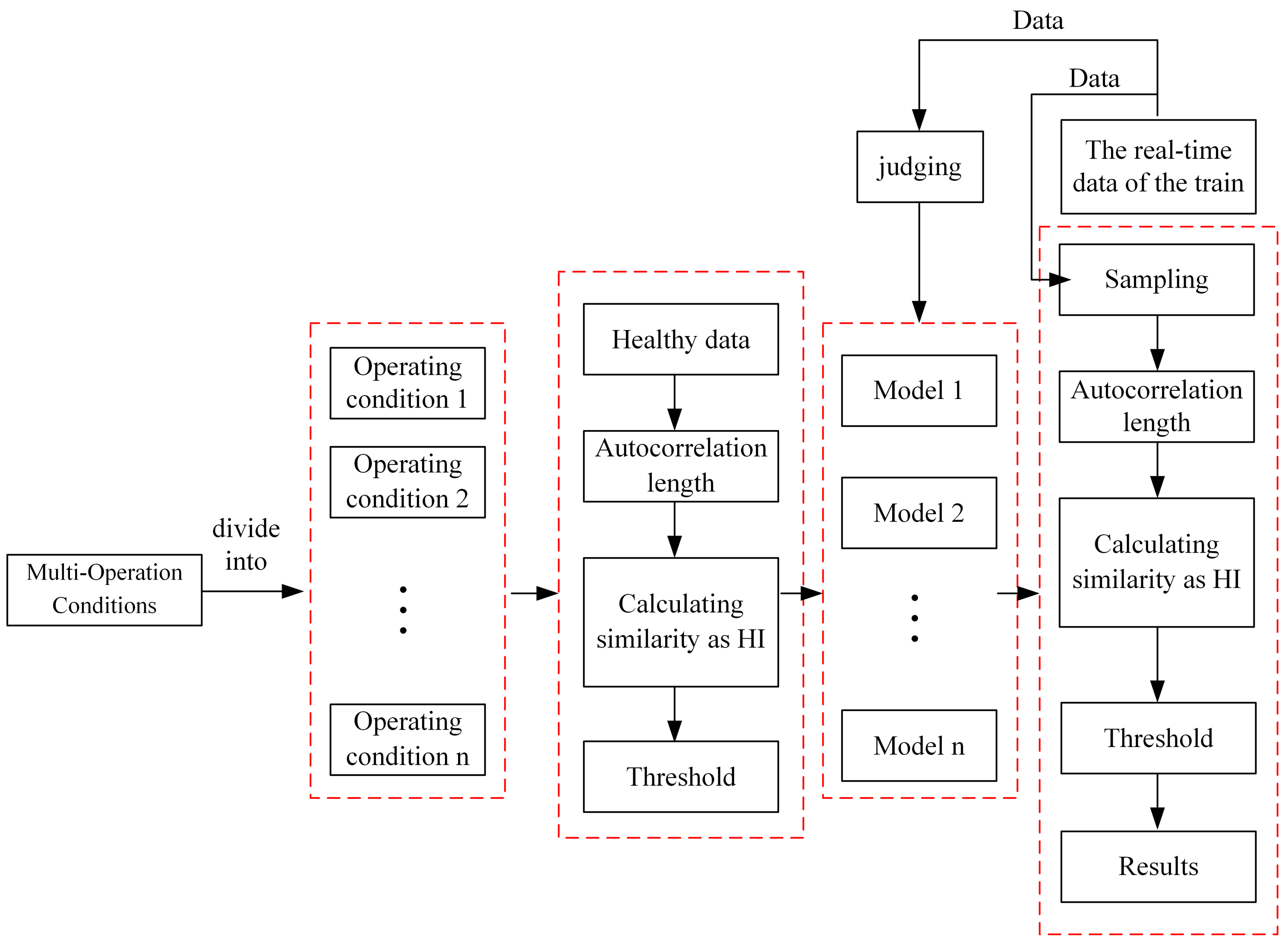
Figure 1 shows the algorithm flow chart of fault detection for the system, which mainly includes the division of multi-operation conditions, autocorrelation analysis, and fault detection. Among them, fault detection includes improved similarity and the setting of the threshold.

2.1. Multi-Operation Conditions

During actual engineering, complex systems are implicated by internal, environmental, and human factors, thus leading to multi-operation conditions. Moreover, the data under different conditions are quite distinct. To tackle this problem, the hypersphere model is applied.

In this paper, a hypersphere model represents the aggregate of all data under an operation condition. The radii of the hypersphere models are different because the data under different operation conditions are distinct. In the hypersphere model, the distance from any position in the space to the center of the sphere denotes the corresponding HI. As shown in Figure 2, three spheres with different radii denote three different operation conditions. Among these, $S_1$, $S_2$, and $S_3$ denote three continuous samples, $O_1$, $O_2$, and $O_3$ are the centers of the three super spheres, and $D_1$, $D_2$, and $D_3$ are the HIs of the system. According to degradation law, the corresponding HI decreases from $S_1$ to $S_2$ and then to $S_3$, that is, $\left(D_1>D_2>D_3\right)$. However, due to discrepancies in the data, $D_2$ > $D_1$, that is, the HI at $S_1$ is smaller than that at $S_2$. As a consequence, the change in the data is not obvious. If these data are directly used without considering multi-operation conditions, it is formidable to obtain the ideal consequences of fault detection.

Generally, two methods are used to tackle the problem of multi-operation conditions. One is used for establishing a general fault detection model, and the other is used for simplifying complex conditions into several simple operation conditions, and then the fault detection model is established separately for each simple operation condition. The crux of the former is to ascertain a general model, which can tackle all operation conditions; the crux of the latter is that the researchers have certain prior knowledge from the historical data of the system. In light of existing experience, the second method is comparatively better applicable. The problem of the former is in dealing with complex operation conditions and data discrepancies caused by different operation conditions, and it is liable to give rise to situations of a low fault detection rate and a high false-positive rate. Consequently, for this paper we selected the second method to solve the problem of multi-operation conditions. In the right half of Figure 1, the current operating condition is judged based on real-time data, and then according to the judgment result, the fault detection model under the current operating condition to be established in the follow-up is switched in time. In addition, the calculated similarity is the HI index.

2.2. Autocorrelation Analysis

The autocorrelation length can be determined by the autocorrelation function. The autocorrelation function is used to measure the correlation degree between the values of a random signal x at any distinct time. The autocorrelation sequence of the random signal $x_q$ at q and the random signal $x_{q+m}$ at $q+m$ can be given by the following equation:

$$R_m=E\left\{x_{q+m}{x}_q^{*}\right\}=E\left\{x_q{x}_{q-m}^{*}\right\}$$

(1)

where $-\infty <q<+\infty$, E represents the expectation operator, m is the lag value and the asterisk denotes complex conjugation. When m is equal to 0, the value of $R_m$ is the largest, because the correlation between two identical signals must be maximum. When m is close to 0, the value of $R_m$ usually decreases.

In general, when the autocorrelation function is adopted to calculate the original correlation, the original data do not need to be normalized.

$${\widehat{R}}_{xx}\left(m\right)=\left\{\begin{array}{c}{\sum }_{q=1}^{V-m-1}\left\{x_{q+m}{x}_q^{*}\right\}m\ge 0\hfill \\ {\widehat{R}}_{xx}^{*}(-m)m<0\hfill \end{array}\right.$$

(2)

where V is the length of the sequence.

The vector c obtained by the autocorrelation analysis can be given by the following equation:

$$c\left(m\right)={\widehat{R}}_{xx}^{*}(m-V)m=1,2,\dots ,2V-1$$

(3)

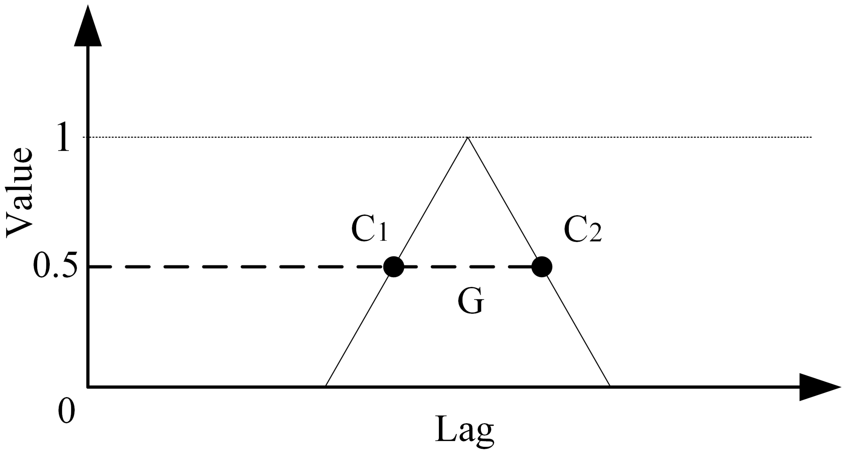
Standardized x means that the obtained value of the autocorrelation function is converted to between 0 and 1 [21]. As shown in Figure 3, suppose that the auto-correlation value of $c_1$ and $c_2$ after standardization is 0.5, and G is the distance between $c_1$ and $c_2$, that is, the auto-correlation length of x. Furthermore, the auto-correlation length is closely bound with the operation conditions. Ordinarily, the auto-correlation length is distinct under different operation conditions, but occasionally there is even a big gap. Therefore, in this paper, a corresponding auto-correlation length is calculated for each condition based on simplifying the intricate condition into several simple mutually exclusive conditions.

To verify the feasibility of determining the data length by autocorrelation analysis, random signals and smooth random signals are taken as examples. First, 150 samples were selected from the random numbers that obey the standard normal distribution to acquire the random signal $Y=(y_1,y_2,\dots ,y_{150})\in N\left(0,1\right)$, as shown in Figure 4a.

Figure 4b shows the autocorrelation diagram of a random signal Y. The ordinate indicates the strength of the correlation, a higher value of which results in a closer correlation. The abscissa represents the delay time of the signal, expressed in lag. Figure 4c shows the $\tilde{c}$ obtained by standardizing c. The corresponding value of the purple dotted line parallel to the x-axis is 0.5. As can be seen from the figure, only one of the 150 points exceeds the purple dotted line, which indicates a value greater than 0.5. Therefore, G is 1. As a matter of fact, regarding the analysis of the characteristics of the random signal itself, since all points of the random signal are independent of each other, there is no interconnection between them, and each point is only related to itself. Consequently, G is also 1.

A moving average filter with a width of 5 was adopted to smooth the signal Y so as to obtain the signal $Y_1$, as shown in Figure 5a. Figure 5b is the autocorrelation diagram of signal $Y_1$, $c_1$ is the ordinate and lag is shown by the abscissa. Figure 5c shows the $\widetilde{c_1}$ obtained by standardizing $c_1$. The purple dotted line parallel to the x-axis is 0.5 above the x-axis. As can be seen from the figure, five of the 150 points exceed the purple dotted line, which indicates a value greater than 0.5. Therefore, the value of G is 5. In light of the characteristics of the signal itself, since $Y_1$ adopts s a moving average filter with a width of 5 to process random signals, G is also 5.

In conclusion, it is feasible and appropriate to determine the length of autocorrelation with the above-mentioned method.

2.3. Fault Detection

Supposing that the Euclidean distance is directly employed to calculate the similarity under the same operation condition, it is liable to detect the fault. The calculation formula is as follows:

$$S=\frac{1}{N}\sum _{i=1}^N{(w_1^i-w_2^i)}^2$$

(4)

where $w_1^i$ is the i-th sample of HI, $w_2^i$ is the i-th unknown sample of HI, and N is the autocorrelation length.

However, the data are very different under different operation conditions. If the similarity is still calculated by Formula (4), it is easy to cause the size of the similarity under different operation conditions to vary greatly. In this way, when multi-operation conditions are continuously switched, operators will not be able to intuitively understand all operation conditions of the system on an interface. Therefore, this paper uses the error percentage between current data and specific health data to replace Euclidean distance and establishes an exponential model. The result of each data point can be controlled between 0 and 1 using this model. Meanwhile, considering that the cumulative sum may enlarge differences between the results, the average value of the exponential model is taken as the final result. This ensures that all similarities under different operation conditions are within the same range. The improved similarity method is expressed by:

$$S=\frac{1}{N}\sum _{i=1}^N{e}^{-{\left(\frac{w_1^i-w_2^i}{w_1^i}\right)}^2}$$

(5)

According to Formula (5), the greater the difference between the two sequences is, the smaller S is. The smaller the difference between the two sequences, the greater S is. Only when the two sequences are identical, S has the maximum value of 1. In short, the larger S is, the healthier the system becomes.

For the setting of a fault threshold, a section of healthy historical data is first selected as the basis, and then the average value $\mu$ and standard deviation $\sigma$ of the data are calculated. Finally, it is only necessary to set the lower limit of the HI, i.e., $\mu -3\sigma$, as the fault threshold because the HI will decline when the system fails.

3. Experimental Verification

3.1. Data Introduction and Operation Condition Division

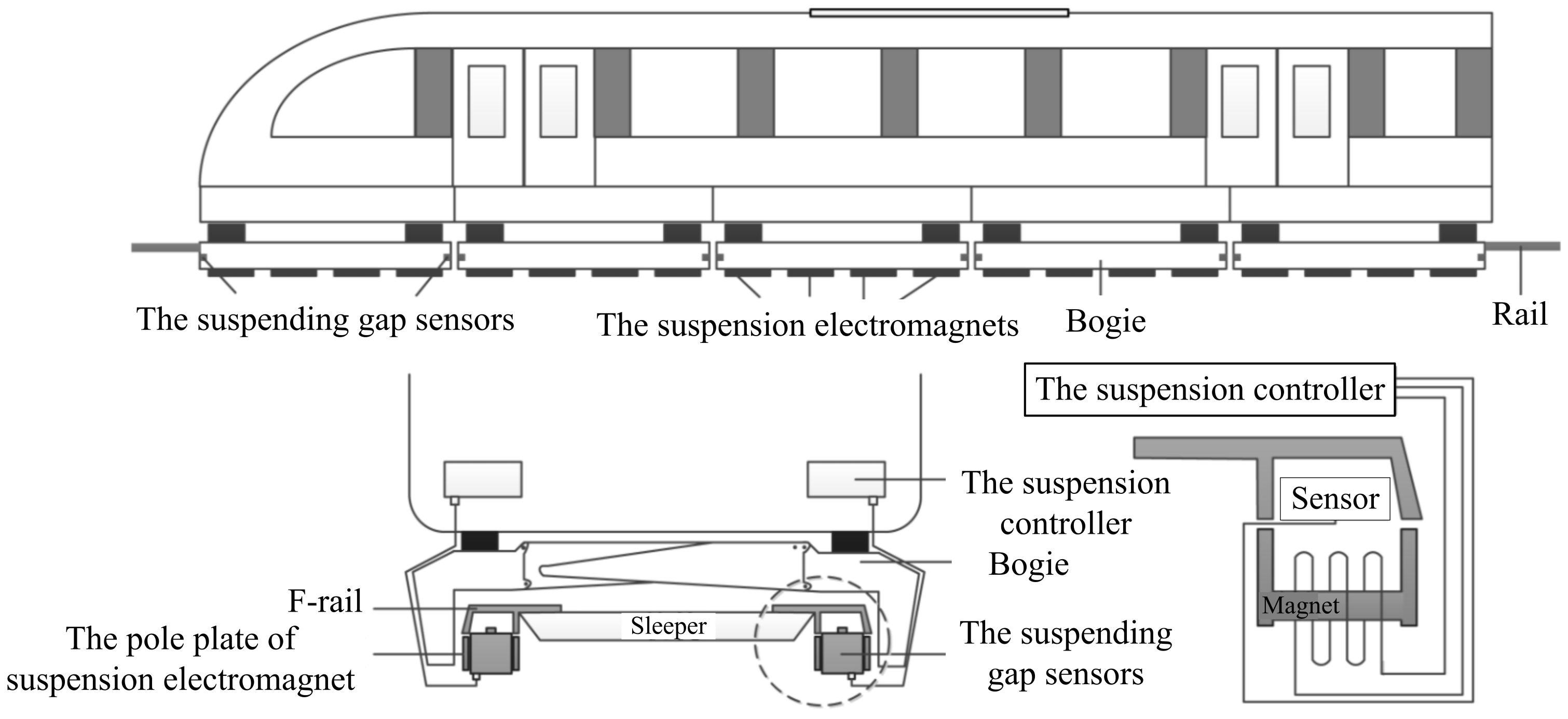
Figure 6 is the schematic diagram of a single-point suspension node. Due to gravity, the carriage and the suspension frame receive a downward force, causing the gap between the electromagnet and the rail to grow. The suspension controller receives the value of the gap from the gap sensor and generates a PWM wave to a power chopper. According to the PWM wave, the power chopper adjusts the current to keep the value of the gap at a fixed value. Therefore, the gap can be applied to determine whether the system has failed. There are 20 suspension points in a carriage (There are 10 suspension nodes on each side and their distribution is symmetrical). If the suspension node fails, the symmetry on both sides loses balance. This will cause the maglev train to not operate safely.

The relevant data of the suspension system were collected by a monitoring suspension unit (MSU) [22]. Figure 7a shows the historical data of a single-point suspension system for one day, which contain an overload fault (a common fault), and the sudden increase of the final gap is caused by the train’s stop. Figure 7b is the enlarged drawing of the fault in the historical data. The suspension node has an overload fault from near $1.391\times {10}^5$ to almost $1.443\times {10}^5$. As can be seen from Figure 7b, when t = 138,800, the suspension gap of the train suddenly increases, but the change is still in the normal range. After 300 sampling times, the system failed to adjust the suspension clearance of the train within the expected value. On the contrary, when t = 139,100, the continued growth of the gap value leads to a collision track of the train, so a fault of the suspension system occurs. In the next 600 sampling times, the acceleration changes sharply and the speed decreases rapidly. After t = 139,700, the train continues to run at a lower and fluctuating speed, and the gap remains unchanged. Then the speed drops to 0 and the system stops. When t = 144,300, the suspension gap reaches the normal value again, and the train restarts. After 100 sampling points under the static suspension, the train starts to accelerate and the system returns to normal running. This is a non-emergency method for the overload fault of the suspension node.

During the actual running of a train, there generally are three possible situations: operating, static suspension, and falling off [23]. However, regarding the suspension system, operating and static suspension are the main operation conditions during use. Therefore, this paper mainly focuses on the operating and static suspension. Moreover, the switching rules of the two operation conditions are established correspondingly [24].

3.2. Experimental Results and Analysis

In light of the autocorrelation analysis, the autocorrelation lengths in operation and in the static suspension condition were 920 and 46, respectively. The data of the initial autocorrelation length in each operation condition were thus chosen as health data. According to Equation (5), the similarity between subsequent data and the health data was calculated. Figure 8 shows the HI curve that resulted from the proposed method. The blue curve indicates the HI of the suspension system when it is under the static suspension, and the red curve indicates the HI of the suspension system during the operating phase condition. In the figure, there is an obvious fault state in the red curve and an apparent abnormal state in the blue curve. Meanwhile, the distinction between the health state, the abnormal state, and the fault state is relatively large.

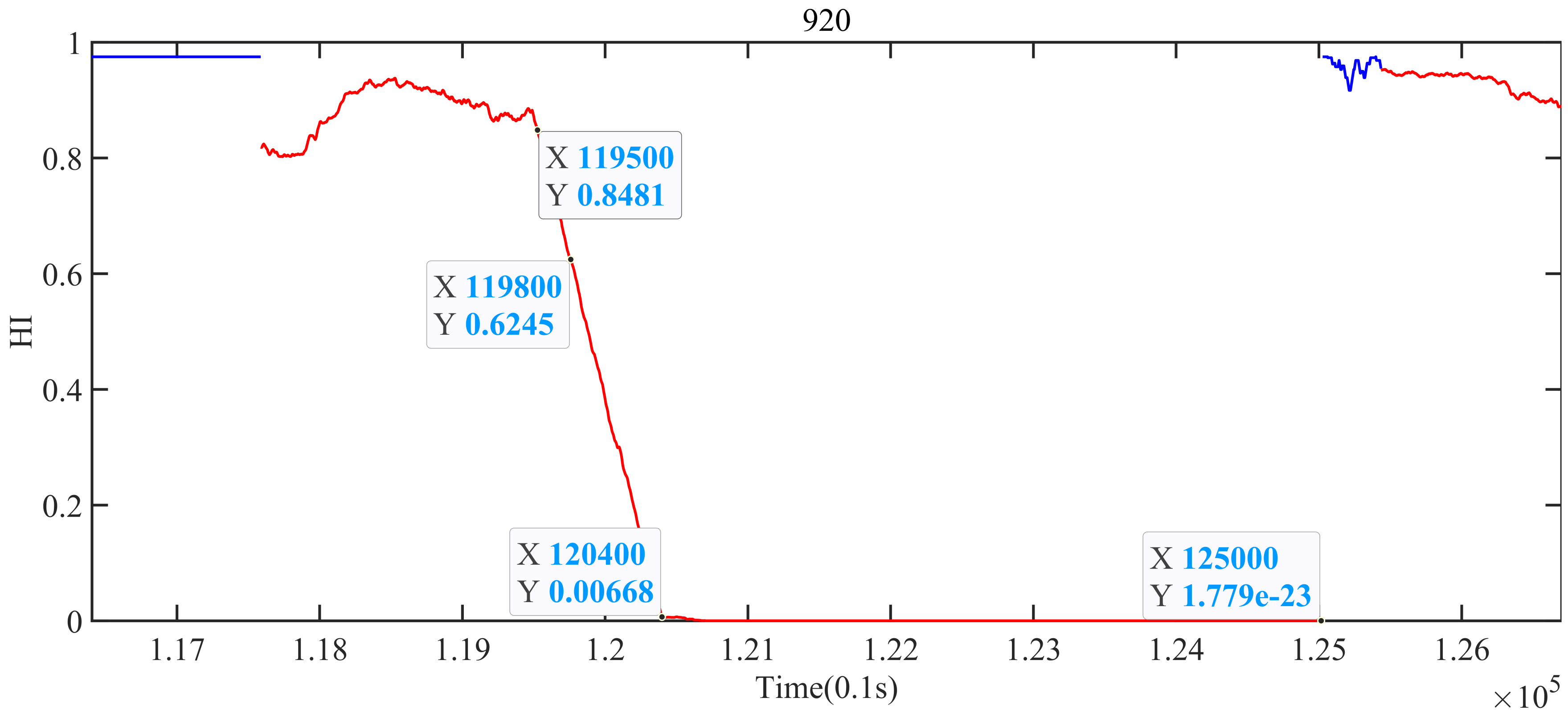
Figure 9 is an enlarged drawing of the fault shown in Figure 8. As shown in Figure 9, the time that the fault happened in the historical data is from 139,100 to 144,300, while in Figure 9, the corresponding fault interval is between 119,800 and 125,000. In Figure 9, when t = 138,800, the suspension gap of the suspension system becomes larger, but it is still in the normal range, and there is no rail crash. However, from 138,800 to 139,100, the gap of the suspension system did not recover to the expected clearance, and the fault occurred at 139,100. Correspondingly, in Figure 9, when $t=\mathrm{119,500}$, the HI of the suspension system belongs to the normal value. However, since t = 119,500, the HI of the system decreases approximately linearly. t = 119,800 is the time when the fault occurs, and the HI of the system at this time is 0.5377. When a fault occurs, the train starts to slow down. After 600 sampling times, that is, when t = 120,400, the train runs at a low speed, but the HI of the suspension system is close to 0. After t = 125,000, the train speed is 0 and the suspension system is restarted. At this time, the suspension system recovers the suspension performance and is under the static suspension. It shows that the proposed method can monitor the HI of the system and detect the fault. Moreover, it can be seen that the HI of the system becomes low before it reaches the threshold value, which has the function of early warning.

Figure 10 shows a comparison of health data and abnormal data under the static suspension. Figure 10a shows health data under a static condition. At this time, the data are 9.29, which is the most ideal. Figure 10b shows the abnormal data under the static suspension. At this time, the data fluctuated greatly and showed instability. Figure 10c shows the HI of abnormal data under the static condition. Since the autocorrelation length under the static suspension condition is 46, the curve in Figure 10c starts from 46. The data in Figure 10b are different from the health data at the beginning, and the HI is about 0.8. The data in the middle tend to be stable and close to the healthy value, and the data in this stage are close to 1. However, in the subsequent data, the suspension gap suddenly increases to 9.8 and remains at that level, then suddenly increases and then jumps back to near the health value. Meanwhile, the HI decreases rapidly and approaches the health threshold. It then suddenly drops again and quickly rises above the health threshold. This process can only be judged as a system exception.

In addition, when the system fails, the similarity curve is extracted, as shown in Figure 11. The intervals of the black line segment and the orange line segment indicate the similarity of the health history data and the test data, respectively. The fault threshold (0.8212) of the similarity is the orange line. In the test data, most of the blue curves are above the threshold, except for some abnormal points (those surrounded by the purple circle in the figure) and the fault points.

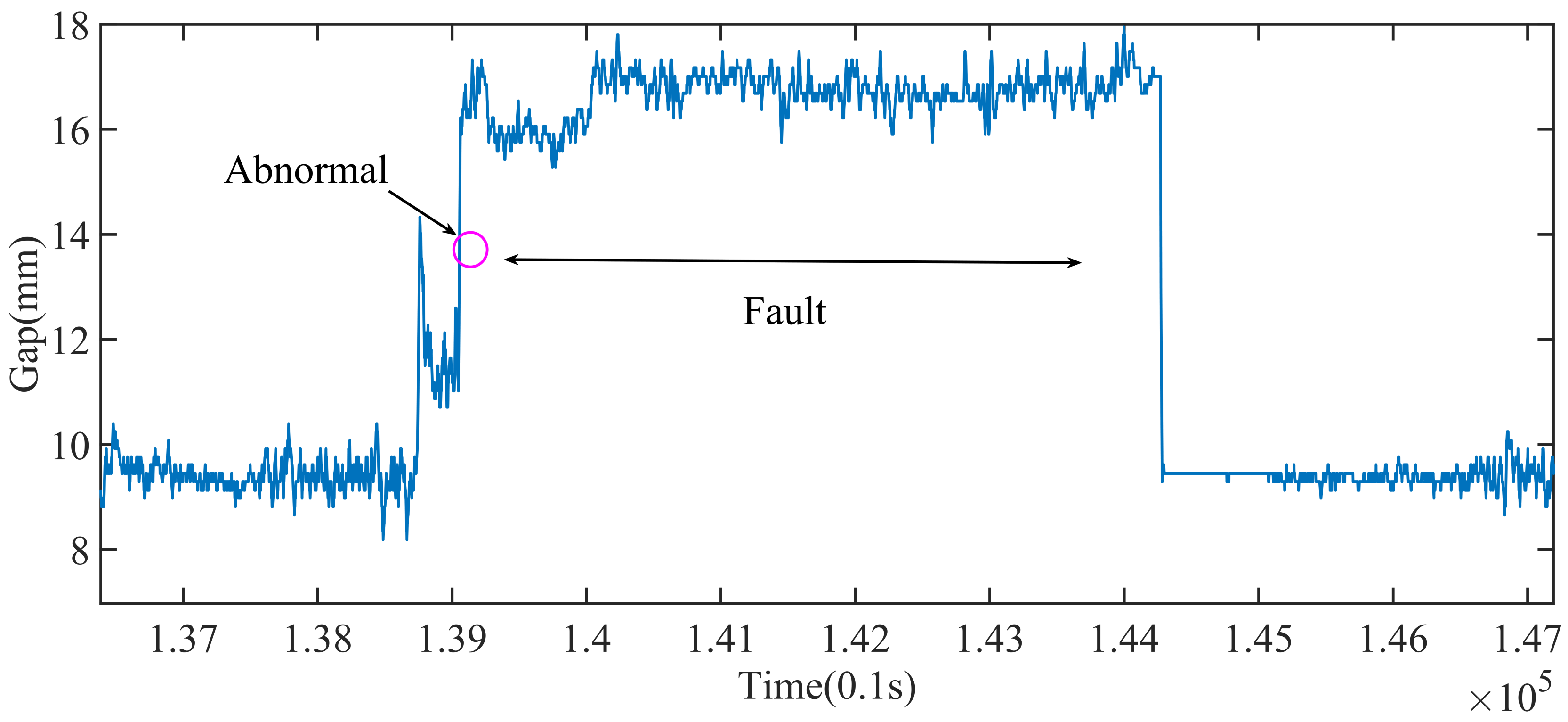
The abnormal points, that is, the position of the purple circle in Figure 11, may need to be analyzed by combining with the data of the gap (shown in Figure 12). In Figure 12, the gap suddenly rises from 10 to 14 mm and then returns to about 12 mm. This is abnormal.

Therefore, this indicates that the proposed method can monitor the HI of the system and detect faults and abnormal behaviors.

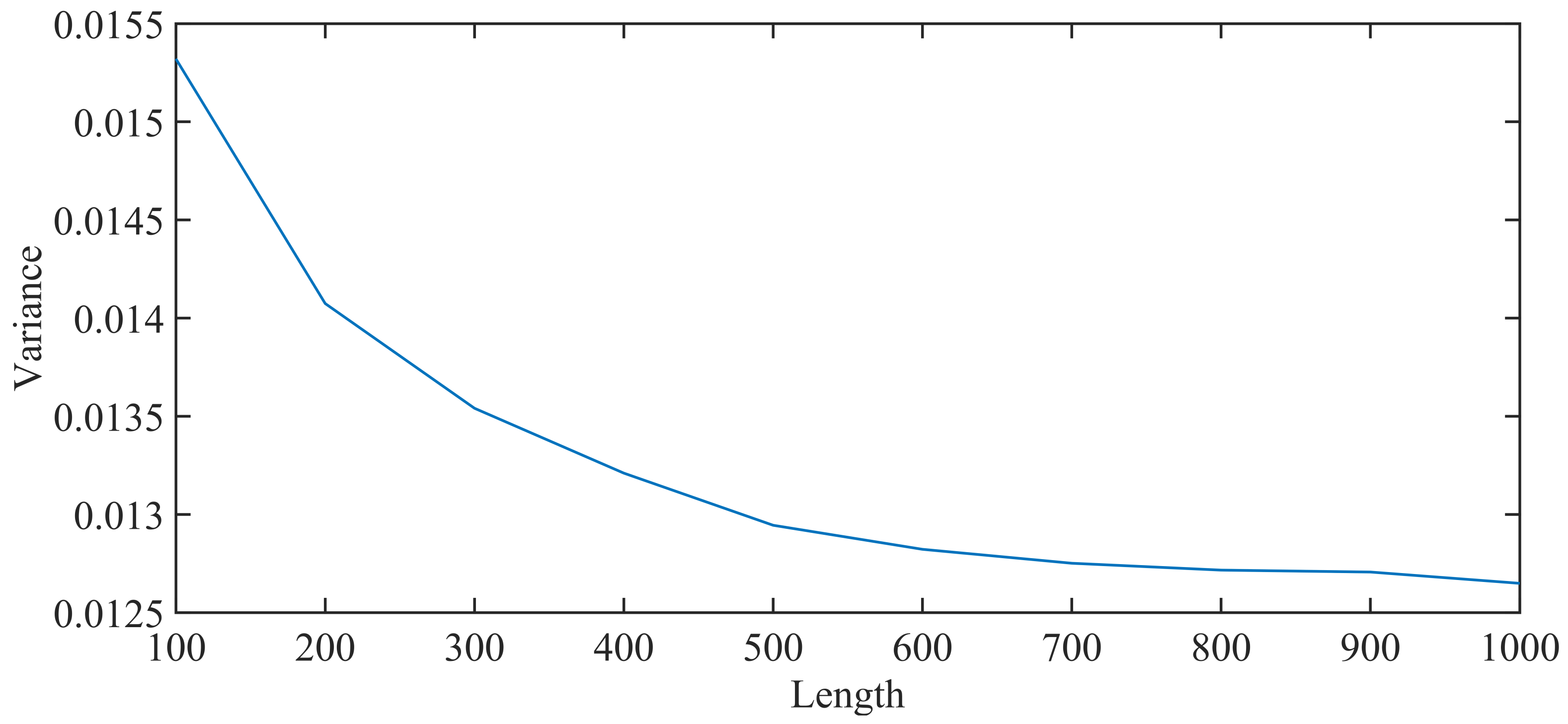
3.3. Effect of Different Data Lengths

The length of data has a great impact on the results. Therefore, this section focuses on the impact of data length. Data are the information that can best reflect the HI of the system, and the length of the data determines the amount of information. If the selected data are short, the information be insufficient, and the HI obtained by calculation will be uncertain, which will lead to the fluctuation of the curve; the less information, the greater the volatility of the curve.

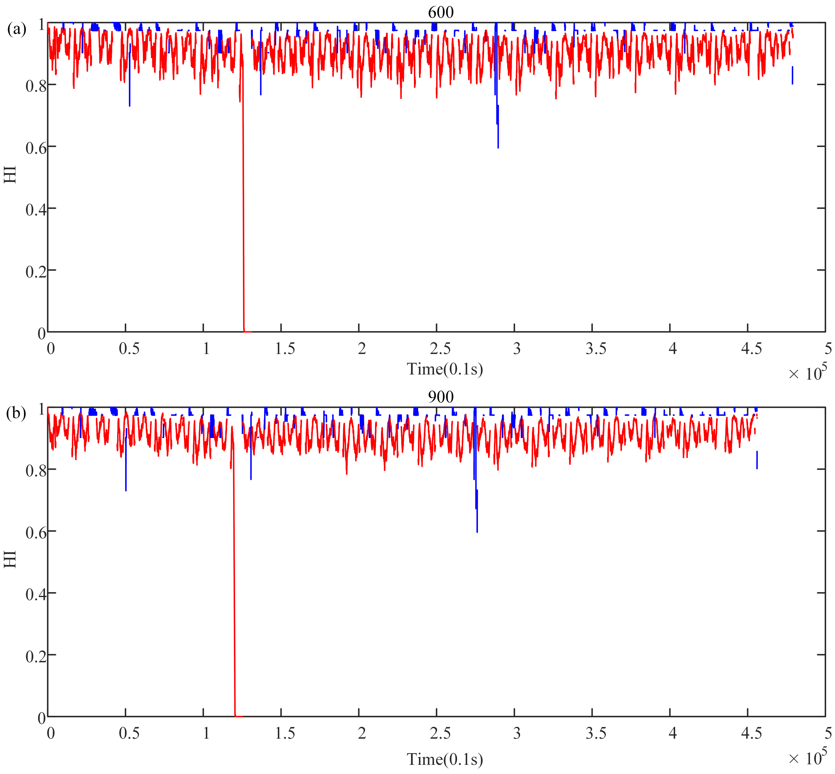
Taking the operating phase as an example, the length under the static suspension condition remains unchanged. Values taken at intervals of 100 during 100 and 1000 are used as the length of the data. Variance is an important index to reflect the volatility of the curve. Figure 13 shows the variance variation diagram of train health during the operating phase. It can be seen from the figure that when the length is 100, the variance is the largest, that is, the volatility is the largest. This means that this length contains the least information. When the length slowly increases to 1000, the variance curve decreases exponentially and tends to be stable when the length is 900, as shown in Figure 14 and Figure 15 (blue indicates the HI of the suspension system when it is under the static suspension, and red indicates the HI of the suspension system during the operating phase). This shows that the information contained in the data begins to meet the needs of health indicators when the data length is 900. However, if we continue to increase the data length, it will not benefit the calculation of HIs but will increase the amount of calculation.

In the experiment, it is suitable to adopt the enumeration method to determine the data length as 900, but if the amount of data is large, thus making the number of enumerations being large, it needs a large amount of calculation and more time to determine the appropriate length. The length determined in this paper is 920, which is close to 900. This shows that the method in this paper can quickly determine the length of the data, avoid a large amount of calculations, and save calculation time.

3.4. Comparison of Methods

To illustrate the effectiveness of the proposed method, three methods based on similarity (labeled as method 1, method 2, and method 3) and a data-driven method (marked as method 4) [22] are used for comparison. Equations (6)–(8) are the calculation equations of method 1, method 2, and method 3, respectively.

$$S=\sum _{i=1}^N{(y_1^i-y_2^i)}^2$$

(6)

$$S=\frac{1}{N}\sum _{i=1}^N{(y_1^i-y_2^i)}^2$$

(7)

$$S=\sum _{i=1}^N{e}^{{-(y_1^i-y_2^i)}^2}$$

(8)

Figure 16 shows the curve obtained by method 1. Green indicates the HI of the suspension system under the static suspension, and red indicates the HI of the suspension system during the operating phase. Although the fault location of the system during the operating phase can be well detected, the abnormal position of the system is not detected and the HI of the health data is close to 0. This is because the Euclidean distance increases the difference between fault data and health data. It is not convenient for operators to intuitively understand the real-time health of the system, especially analyzing the impact of the human illegal operation on the system.

Figure 17 is a curve obtained by method 2. Green indicates the HI of the suspension system under the static suspension, and red indicates the HI of the suspension system during the operating phase. Compared with Figure 16, although the fault position during the operating phase and the abnormal position under the static suspension can be well detected, the HI of the health data is still close to 0. This is not convenient for operators to intuitively understand the real-time health of the system.

It can be seen from Figure 16 and Figure 17 that, although the cumulative differences caused by summation are reduced by means of the average value, the influence of the Euclidean distance on the increase of data differences is still not well improved.

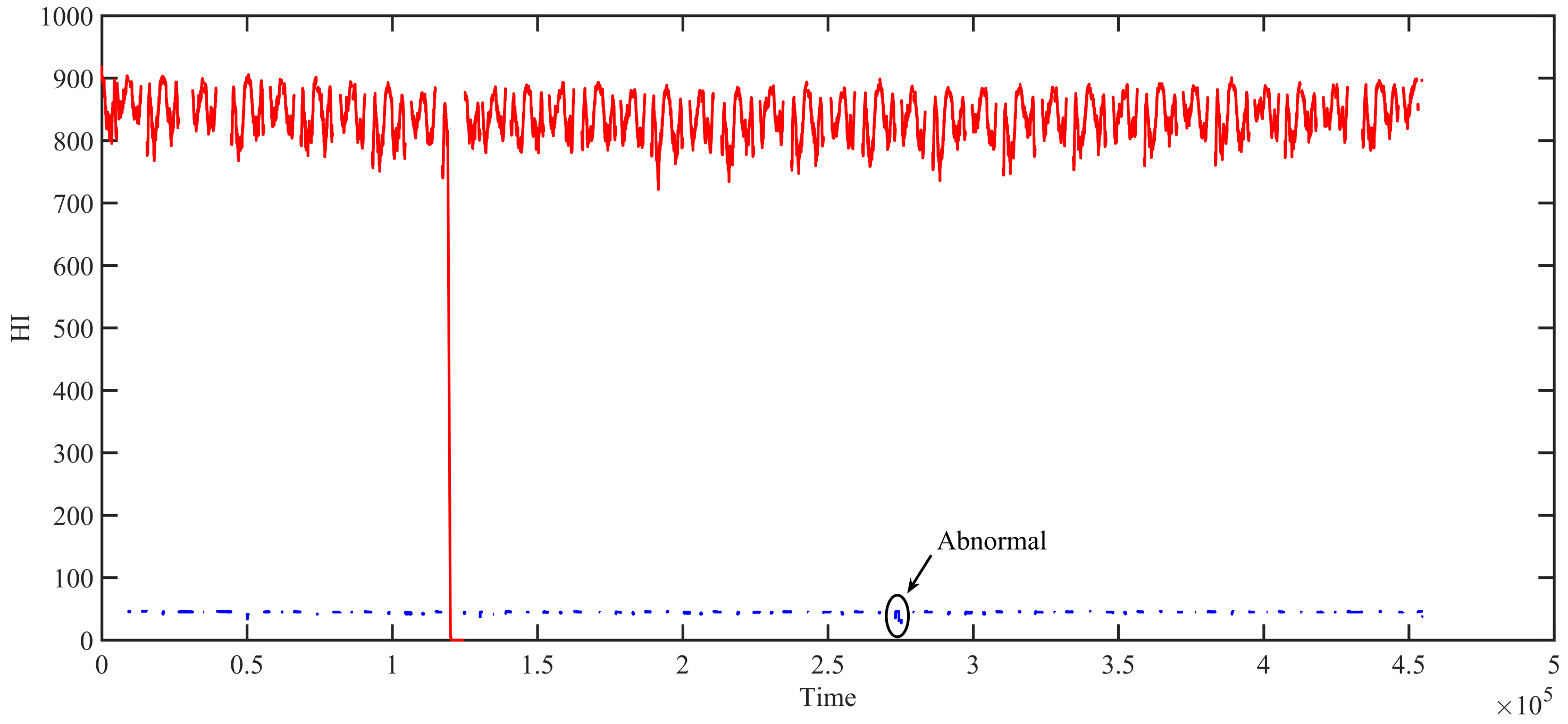
Figure 18 shows the curve obtained by method 3. Green indicates the HI of the suspension system when it is suspended at rest, and red indicates the HI of the suspension system during the operating phase. There is a big difference between the HI during the operating phase and the static suspension. The HI during the operating phase is between 800 and 900, while the HI under the static suspension is within 100. In the figure, the big difference between the red curve and the blue curve is caused by the cumulative summation. Although the HI of the system during the operating phase can be intuitively understood through Figure 18, it is difficult to understand the HI of the system under the static suspension, and especially during the abnormal state, such as the part surrounded by black oval lines in the figure.

Figure 8 shows the curve obtained by the method proposed in this paper. As can be seen, the obtained curve can not only detect faults or abnormal states under different operation conditions but also observe the change of HI at different times. In addition, it can correctly and stably reflect the HI of the system.

It can be seen from Figure 8 and Figure 18 that although the exponential model can reduce the impact of data differences, summation still brings cumulative differences. Furthermore, the influence of cumulative differences can be effectively improved by means of the average value.

Although method 4 can detect the fault when it occurs, the method cannot reflect the state of the system stably, and part of the fault state is even shown as a healthy state during the fault’s occurrence.

To sum up, the method in this paper can not only quickly select the length of the data under the condition that the amount of information is sufficient, so as to reduce the amount of calculation as much as possible, but also unify the HI under different operation conditions to the same interface and detect faults or abnormal states, so that operators can intuitively understand the HI of the system. Additionally, it can correctly and stably reflect the HI of the system. Therefore, the method proposed in this paper is better than the methods mentioned above.

4. Conclusions

To resolve the problems of fault detection for complex systems, this paper proposes a fault detection method, which is based on correlation analysis and improved similarity. Firstly, based on existing historical data, complicated operation conditions are simplified into several simple operation conditions. Secondly, under the condition that the amount of information is sufficient, the length of the data determined via the correlation length is applied to calculate the similarity. This can reduce the amount of calculation as much as possible. Thirdly, to resolve the problem that the range of similarity under multi-operation conditions is different, an improved similarity method is proposed to make the range of similarity under different operation conditions the same, so that operators can intuitively understand the HI of the system. Finally, the proposed method was applied to the suspension system of the maglev train. The results indicate that the proposed method can not only detect faults or abnormal states but also observe the HI changes of the system under different operation conditions. Moreover, the method proposed in this paper was found to be better than the methods mentioned in Section 3.

Throughout this paper, it has been concluded that the proposed method is applicable and effective in fault detection for the suspension system of maglev trains. However, the real-time performance of this method is not high. As a result, this method may not be able to detect faults in real time. In future work, improving the real-time performance of the method will be an important research focus. In addition, future work will also consider: (1) locating the root cause in faulty suspension systems; (2) developing methods for reducing the fluctuation caused by environmental factors, human factors, and system factors.