The Short-Term Forecasting of Asymmetry Photovoltaic Power Based on the Feature Extraction of PV Power and SVM Algorithm

Abstract

To improve forecasting accuracy for photovoltaic (PV) power output, this paper proposes a hybrid method for forecasting the short-term PV power output. First, by introducing the noise level, an improved complementary ensemble empirical mode decomposition (EEMD) with adaptive noise (ICEEMDAN) is developed to determine the ensemble size and amplitude of the added white noise adaptively. ICEEMDAN can change PV power output with non-symmetry into intrinsic mode functions (IMFs) with symmetry. ICEEMDAN can enhance the forecasting accuracy for PV power by IMFs with physical meaning (not including spurious modes). Second, the selection method of relative modes (IF), which is determined by the comprehensive factor, including the shape factor, crest factor and Kurtosis, is introduced to adaptively classify the IMFs into groups including similar fluctuating components. The IF can avoid the drawbacks of threshold determination by an empirical method. Third, the modified particle swarm optimization (PSO) (MPSO) is proposed to optimize the hyper-parameters in the support vector machine (SVM) by introducing the piecewise inertial weight. MPSO can improve the global and local search ability to make the particles traverse the global space and strengthen the performance of local convergence. Finally, the proposed method (ICEEMDAN-IF-MPSO-SVM) is used to forecast the PV power output of each group individually, and then, the single forecasting result is reconstructed to obtain the desired forecasting result for PV power output. By comparison with the other typical methods, the proposed method is more suitable for forecasting PV power output.

1. Introduction

Recently, with the rapid development of science and technology, energy demand has become more and more important [1,2]. Many countries have increasing requirements for energy. Conventional energy such as coal, petroleum and gas do not meet the requirements. In comparison with these energy resources, presenting the advantages of cleanliness, good potential, extendibility and universality, solar power is the one of most desired types of energy among energy resources. In many countries, some large-scale photovoltaic (PV) plants have been developed to reduce environmental pollution. However, PV generation has the drawbacks of intermittence and fluctuation, and being subject to ungovernable solar irradiance and metrological factors, such as wind speed, temperature, humidity and dew retting [3,4]. It also brings new challenges for guaranteeing the stable operation of the power system. Furthermore, the accurate prediction of PV power generation can improve the reliability of the power system, increase the penetration of PV power and decrease the uncertainty of PV power in the power grid [5]. Thus, it is an important task to develop accurate forecasting technology for PV power output.

Several methods have been introduced to forecast PV power output. In the early stage, the time series method has been widely used to forecast PV power output [6,7]. However, the forecasting accuracy is low due to the instability of meteorological conditions. Afterwards, with the development of artificial intelligence (AI), the problem of the low forecasting accuracy can be improved effectively. The technology is widely used in lots of domains due to its robustness [8,9,10]. Likely, many models have also been developed to forecast PV power output. The artificial neural network (ANN) is one of the most outstanding models [11,12,13]. However, when a large neural network is designed, the forecasting accuracy often is poor, and it consumes too much time. Moreover, the ANN also lacks the determined guidance of the hidden layers, numbers and activation functions [14,15].

Fortunately, machine learning based on the support vector machine (SVM) has been proved to be an effective tool for obtaining better forecasting speed and accuracy for non-linear solar power output [16,17]. To design an SVM, the optimal mechanism, which mainly includes a genetic algorithm (GA) [18], grid search (GS) [19] and particle swarm optimization (PSO) [20], is often performed to optimize the hyper-parameters such as the penalty parameter $C$ and the epsilon parameter $\epsilon$. Among them, PSO is the most promising. However, PSO also has some drawbacks, such as pre-mature convergence and locally optimal solutions. Afterwards, the inertia weight is introduced to enhance the optimal ability [21]. Unfortunately, the inertia weight is a constant. Then, a dynamic inertia weight is introduced to obtain a better optimal result [22]. Because the inertia weight changes linearly with the iteration number, it does not realize that a large inertia weight is used to enhance the global search ability in the early stage, and a small inertia weight is determined to enhance the local search ability and convergence speed. Thus, determining the inertia weight suitable for improving the optimal performance of PSO is a key task.

Moreover, in recent years, forecasting models based on hybrid approaches have been developed to forecast PV power output and energy demand, such as wave and ocean energy generation systems [23,24]. The hybrid approaches can obtain better forecasting accuracy. The most representative methods were based on wavelet analysis [25,26], empirical mode decomposition (EMD) [27,28,29] and variational mode decomposition [30], respectively. However, the wavelet basis function needs pre-definition and is non-adaptive in nature. EMD is prone to mode mixing. Afterwards, multivariate EMD was proposed and applied in the forecasting domain [31,32,33]. However, the mode mixing still could not be resolved. The penalty factor and mode number of variational mode decomposition (VMD) are difficult to determine, decreasing the decomposition effectiveness for PV power. The ensemble EMD (EEMD) [34] was developed by adding Gaussian white noise into the original signal to solve the problem of mode mixing. However, this approach also introduces a new problem. The intrinsic mode functions (IMFs) contain the residue white noise, and the different realizations of signal and noise may produce spurious modes. The complementary EEMD with adaptive noise (CEEMDAN) [35] was then proposed to solve the problems of residue noise and spurious modes. Forecasting models based on CEEMDAN are widely used in the forecasting domain such as for rainfall forecasts and wave height forecasting [36,37]. However, CEEMDAN involves two critical parameters, namely, the amplitude of the added white noise (NA) and the number of ensemble trials (EN). If the NA is too small, then it is difficult to avoid mode mixing. However, if the NA is too large, a very high EN is needed to eliminate the residue noise. Hence, it is a challenge to determine the NA and EN. Huang et al. [34] determined the two critical parameters by an empirical method. However, it is unsuitable for decomposing signals for all cases. Zhang et al. [38] propose using the correlation coefficients between the IMFs and the original signal to determine the suitable EN. Niazy et al. [39] employed the relative root-mean-square error (RMSE) to determine the appropriate NA. However, these methods do not select the noise level. Thus, it is very urgent to develop a suitable method to determine the proper parameters (NA and EN) to decompose PV power output. Papers indicate [40,41] that among the hybrid methods based on EEMD, EEMD is used to decompose the PV power data into specified groups based on the frequency characteristic of the IMFs. Each group stands for the feature fluctuation components of the original PV power output. The key task of the determined specified group is to look for the reasonability threshold. Generally, the determination of the threshold often depends heavily on experience. This may bring a potential risk of the wrong determination of frequency components for making the different fluctuational components mixed into a group. Finally, the prediction accuracy when each group is considered as the “original” PV power output is important. Thus, it also necessary to develop an adaptive method to distinguish the effective frequency components to enhance the prediction accuracy.

To solve the above-mentioned problem, this paper develops a hybrid method based on an improved CEEDMAN (ICEEMDAN), the identification of specified IMFs and the SVM. This method applies the ICEEMDAN to decompose the PV power output into a set of IMFs, the IMFs are divided into different groups, each group is considered as the “original” PV power output, and each “original” PV power output is forecast. Finally, the predicted result is reconstructed to obtain the final PV forecasting. Thus, the main contributions with regard to the previous work are as follows:

(1)

The effective decomposition of the original PV power output.

In this paper, the two critical parameters of CEEMDAN, which include the amplitude of the added white noise and ensemble size, are optimized by the defined concept of the noise level. The improved CEEMDAN (ICEEMDAN) can suppress the spurious mode in traditional CEEMDNA decomposition and further enhance the decomposition effectiveness.

(2)

The reasonable identification of specified IMFs.

The identified method based on the correlation between the PV power output data and each IMF is proposed to divide the IMFs into the corresponding groups adaptively. This is an adaptive method. This method can avoid the mixing of the different fluctuation components in same-group IMFs.

(3)

The parameter optimization of the SVM.

The modified PSO (MPSO) based on the piecewise inertia weight is proposed to optimize the parameters in the SVM. The MPSO can realize that a large inertia weight is used to enhance the global search ability in the early stage, and a small inertia weight is determined to enhance the local search ability and convergence speed.

(4)

The reconstruction of the forecasting result.

Each group’s IMFs are considered as the “original” PV power and forecast with the SVM. The forecasting result of each group is reconstructed to obtain the final PV power forecasting output.

The proposed method (ICEEMDAN-IF-MPSO-SVM) is used to forecast the PV power output, and the result indicates that the proposed method has a better forecasting performance compared with the traditional methods.

The rest of the paper is organized as follows. Section 2 describes the related work including the signal decomposition method and the forecasting method for PV power output; Section 3 presents the proposed method; Section 4 discusses the comparison of the forecasting results; Section 5 is the conclusion.

2. Related Work

2.1. CEEMDAN Algorithm

Although EEMD [34] can overcome the drawback of mode mixing in EMD, it also contains two drawbacks: the residue noise and the spurious mode. Afterwards, the CEEMDAN [35] is introduced to alleviate the above-mentioned problems. The following is the principle of CEEMDAN:

(1)

Obtain the noisy signal $x^i$; $x^i=x+{\omega }_0{\xi }^i\left(i=1,\cdots ,N\right)$, where ${\xi }^i$ is the added white noise with unit variance, ${\omega }_0$ is the corresponding coefficient, and $x$ is the original signal;

(2)

Extract the first IMF ($c_1^i$) from each noisy signal $x^i$ with EMD;

(3)

Obtain the first IMF ($c_1$) by taking the average of each $c_1^i$;

$$c_1=\frac{1}{N}{\displaystyle \sum }_{i=1}^N{c}_1^i$$

(1)

(4)

Obtain the first residue: $r_1=x-c_1$;

(5)

Decompose $r_1+w_1{E}_1\left({\epsilon }^i\right)$ with the EMD algorithm, and extract the first IMF to obtain the second IMF ($c_2$), where $w_1$ means the coefficient of the added white noise, and the operator $E_m(\cdot )$ indicates the $m$-th IMF with EMD;

$$c_2=\frac{1}{N}{\displaystyle \sum }_{i=1}^N{E}_1\left(r_1+w_1{E}_1\left({\epsilon }^i\right)\right)$$

(2)

(6)

Compute the $m$-th residue mode ($m=2,\dots ,K$), and extract the first IMF to generate the $\left(m+1\right)$-th IMF with Equation (3);

$$c_{m+1}=\frac{1}{N}{\displaystyle \sum }_{i=1}^N{E}_1\left(r_m+w_m{E}_m\left({\epsilon }^i\right)\right)$$

(3)

(7)

Repeat the above steps until the residue $\mathrm{R}$ contains fewer than two extrema;

$$\mathrm{R}=\mathrm{x}-{\displaystyle \sum }_{m=1}^K{c}_k$$

(4)

Finally, the signal $\mathrm{x}$ can be written as:

$$\mathrm{x}={\displaystyle \sum }_{m=1}^K{c}_k+R$$

(5)

Here, $K$ indicates the decomposing number of the IMF.

2.2. SVM Algorithm

The support vector machine (SVM) is an effective tool for tackling the regression and class problem in machine learning. The SVM derives from an optimization problem for the non-linear dataset:

$$\underset{w,b,{\xi }^{(*)}}{\min }\frac{1}{2}{\Vert w\Vert }^2+C{\displaystyle \sum _{i=1}^l\left({\xi }_i+{\xi }_i^{*}\right)}$$

(6)

subject to:

$$\left(\left(w\cdot \Phi \left(x_i\right)\right)+b\right)-y_i\le \epsilon +{\xi }_i,\hspace{1em}i=1,\dots ,l$$

$$y_i-\left(\left(w\cdot \Phi \left(x_i\right)\right)+b\right)\le \epsilon +{\xi }_i^{*},\hspace{1em}i=1,\dots ,l$$

$${\xi }_i^{*}\ge 0i=1,\dots ,l$$

where $l$ refers to the sample size, $\left(x_1,y_1\right)\dots \left(x_l,y_l\right)$ is the group of input and output vectors, $w$ refers to the weight factor, $b$ refers to the threshold value, $C$ indicates the penalty parameter, the kernel function $\Phi$ maps the input samples to higher space, $\epsilon$ means the epsilon parameter, and ${\xi }_i\mathrm{and}{\xi }_i^{*}$ are the upper and lower training errors, respectively. At present, the typical kernel functions include the radial basis function (RBF), polynomial function and linear function [25,26,27]. They are used to map non-linear features between the input and feature space. This paper employs the RBF as the kernel function in the SVM, and the RBF is expressed as follows:

$$k\left(x_i,x_j\right)=exp{\left(\frac{\Vert x_i-x_j\Vert }{2{\gamma }^2}\right)}^2$$

(7)

2.3. PSO Algorithm

PSO is developed through the simulation of the natural flocking and swarming behavior of birds and insects. Here, the flying space of the birds refers to the search space of the resolution problem. Then, each bird is considered as a particle with no mass and volume. Furthermore, each particle refers to a possible solution. During the search process, each particle adjusts its flying velocity and position according to flying experience and the experiences of the other companion particles. Thus, the optimization problem can be solved by the optimization solution. It is assumed that there is a swarm with size N, and each particle has the own position and velocity. The velocity $v_{ij}$ and position $x_{ij}$ of the $i$-th particle in the $j$-th space can be updated:

$$v_{ij}\left(t+1\right)=w\cdot v_{ij}\left(t\right)+c_1{r}_{1j}\left(t\right)\left(p_{ij}\left(t\right)-x_{ij}\left(t\right)\right)+c_2{r}_{2j}\left(t\right)\left(p_{gj}\left(t\right)-x_{ij}\left(t\right)\right)$$

(8)

$$x_{ij}\left(t+1\right)=x_{ij}\left(t\right)+v_{ij}\left(t+1\right)$$

(9)

where $w$ refers to the inertia weight, $t$ indicates the iteration times $i=1,\dots ,N$ and $j=1,\dots ,N$, and $D$ refers to the space dimension. The $c_1$ and $c_2$ are constants and indicate the influence level for the particle from social and individual cognition. The $r_{1j}\left(t\right)$ and $r_{2j}\left(t\right)$ refer to random numbers, which are within [0, 1] and obey a uniform distribution. The ${\mathit{x}}_{\mathit{i}}=\left(x_{i1},x_{i2},\cdots ,x_{iD}\right)$ vector is the potential solution. The position ${\mathit{p}}_{\mathit{i}}=\left(p_{i1},p_{i2},\cdots ,p_{iD}\right)$ and ${\mathit{P}}_{\mathit{g}}=\left(p_{g1},p_{g2},\cdots ,p_{gD}\right)$ indicate that the $i$-th particle experiences the best local position and global position during the flight, respectively.

3. Proposed Work

3.1. Effective Decomposition for PV Power

Subjected to ungovernable metrological factors, PV power output has the drawbacks of intermittence and fluctuation. When traditional EMD is used to decompose PV power output, the related modes cannot be identified effectively due to mode mixing. CEEMDAN can solve the problem of mode mixing. However, the determination of two critical parameters, which are the amplitude of the added white noise (NA) and ensemble size (EN), is not specifically guided. It follows that if the NA is too small, then mode mixing in EMD is difficult to eliminate, and if the NA is too large, a sufficient EN is needed to eliminate the residue noise. It also increases the computational cost. In addition, if the two critical parameters are not suitable to determine, the decomposed result contains a spurious mode because of the interaction between the PV power output and the added noise. The spurious mode, which has no physical meaning, cannot reflect the component information of PV power. To make the decomposition IMFs with CEEMDAN be physically meaningful, this paper introduces the idea of the noise level to determine the two critical parameters (NA and EN).

Assume that the CEEMDAN can decompose the PV power into a set of IMFs as shown in Equation (10):

$$\mathrm{CEEMDAN}\left(x\left(i\right),\mathrm{NA},\mathrm{EN}\right)={\displaystyle \sum _{m=1}^N{c}_k\left(i\right)}+R_N$$

(10)

where $x\left(i\right)$ refers to the PV power output, $N$ refers to the number of IMFs, $c_k\left(i\right)$ refers to the $k$-th IMF, and $R_N$ refers to the residue.

To decrease the computational cost, the EN is set as the smallest trail (two trails).

For the NA determination, the noise level $L_k$ is developed to obtain the optimal decomposition with CEEMDAN. The noise level is developed to decompose the PV power with CEEMDAN under each noise level (as shown in Equation (11)):

$${\mathrm{NA}}_k=L_k\sigma \hspace{1em}\left(k=1,2,\dots ,M\right)$$

(11)

where $\sigma$ refers to the standard deviation of the PV power, and $L_k$ refers to the noise level. The correlation coefficient is calculated between each IMF and the PV power under each noise level decomposition as shown in Equation (12):

$$\mathrm{CC}\left[\begin{array}{cccc}\left({\mathrm{c}}_{11}\left(i\right),x\left(i\right)\right)& \left({\mathrm{c}}_{12}\left(i\right),x\left(i\right)\right)& \cdots & \left({\mathrm{c}}_{1\left(N_1-1\right)}\left(i\right),x\left(i\right)\right)\\ \left({\mathrm{c}}_{21}\left(i\right),x\left(i\right)\right)& \left({\mathrm{c}}_{12}\left(i\right),x\left(i\right)\right)& \cdots & \left({\mathrm{c}}_{2\left(N_2-1\right)}\left(i\right),x\left(i\right)\right)\\ ⋮& ⋮& ⋮& ⋮\\ \left({\mathrm{c}}_{M1}\left(i\right),x\left(i\right)\right)& \left({\mathrm{c}}_{12}\left(i\right),x\left(i\right)\right)& \cdots & \left({\mathrm{c}}_{M\left(N_M-1\right)}\left(i\right),x\left(i\right)\right)\end{array}\right]=\left[\begin{array}{cccc}{\mathrm{C}}_{11}& {\mathrm{C}}_{12}& \cdots & {\mathrm{C}}_{1\left(N_1-1\right)}\\ {\mathrm{C}}_{21}& {\mathrm{C}}_{22}& \cdots & {\mathrm{C}}_{2\left(N_2-1\right)}\\ ⋮& ⋮& ⋮& ⋮\\ {\mathrm{C}}_{M1}& {\mathrm{C}}_{M2}& \cdots & {\mathrm{C}}_{M\left(N_M-1\right)}\end{array}\right]$$

(12)

where ${\mathrm{C}}_{M\left(N_M-1\right)}$ refers to the correlation coefficient between the $\left(N_M-1\right)$-th IMF and PV power under the $M$-th noise level. If the decomposition effect under a noise level is better than that under the other noise level, the correlation coefficient between each IMF and PV power is also bigger than that under the other noise level. Here, the decomposition effectiveness is reflected by averaging the correlation coefficient under each noise level, as shown in Equation (13).

$$m{e}_k=\mathrm{mean}\left({\mathrm{C}}_{k1},{\mathrm{C}}_{k2},\dots ,{\mathrm{C}}_{k\left(N_k-1\right)}\right)\hspace{1em}\left(k=1,2,\dots ,M\right)$$

(13)

where $m{e}_k$ refers to the mean of the correlation coefficients under the $k$-th noise level. In addition, the IMF number can also reflect the decomposition effectiveness. Theoretically, when the signal includes the specified frequency components, CEEMDAN decomposes the signal into a determined number of IMFs. The number is consistent with the number of the components. Each IMF includes a kind of frequency information. However, if there is a spurious mode in the decomposition result, the IMF number should be more than the number of the theoretical IMFs. It indicates that the smaller the IMF number is, the better the decomposed effectiveness is.

Thus, the comprehensive evaluation criterion for decomposition effectiveness can be obtained by combing the $m{e}_k$ with the decomposition number (as shown in Equation (14)).

$$c{r}_k=N_k/m{e}_k\left(k=1,2,\dots ,M\right)$$

(14)

If the $c{r}_k$ under the $k$-th noise level is the smallest:

$$k_{opt}=argmin\left(c{r}_k\right)$$

(15)

The amplitude of the added white noise (NA) can be also determined.

$${\mathrm{NA}}_{k_{opt}}=L_{k_{opt}}\sigma$$

(16)

Finally, the PV power can be decomposed with CEEMDAN by the following expression.

$$\mathrm{CEEMDAN}\left(x\left(i\right),\sigma L_{k_{opt}},2\right)={\displaystyle \sum _{m=1}^N{c}_k\left(i\right)}+R_N$$

(17)

3.2. Selection of Related Modes

To enhance the forecasting accuracy for PV power, the identified method of the related mode is developed to combine the IMFs into a given group to obtain the consistent components of the PV power.

If the IMFs include similar fluctuations of PV power output, the corresponding waveforms are also similar. Based on this principle, this paper develops an adaptive method to identify the IMFs. Firstly, Equation (18) is used to obtain the modified IMF (MIMF).

$$\begin{array}{c}{\mathrm{MIMF}}_1{=\mathrm{IMF}}_1\hfill \\ {\mathrm{MIMF}}_2{=\mathrm{IMF}}_1{+\mathrm{IMF}}_2\hfill \\ {\mathrm{MIMF}}_3{=\mathrm{IMF}}_1{+\mathrm{IMF}}_2{+\mathrm{IMF}}_3\hfill \\ ⋮\hspace{1em}\hspace{1em}\hspace{1em}\hspace{1em}\hspace{1em}\hspace{1em}\\ {\mathrm{MIMF}}_N{=\mathrm{IMF}}_1+{\mathrm{IMF}}_2+{\mathrm{IMF}}_3\dots +{\mathrm{IMF}}_{\mathrm{N}}\hfill \end{array}$$

(18)

Assume that the first N number of the IMFs are similar. It means that the MIMF_N contains similar fluctuation components. If another fluctuation component is introduced into MIMF_(N+1), the waveform between the MIMF_N and MIMF_(N+1) is different, obviously. It is illustrated that if a kind of fluctuation component is mixed into that of another component, the waveform of the adjacent MIMF must be changed.

Here, the comprehensive factor (CF) is developed to identify the difference in adjacent MIMFs (as shown in Equation (19)). The CF includes three evaluated indexes: the shape factor, crest factor and kurtosis (as shown in

Table 1. Evaluated index of waveform fluctuation.

Number	Statistical Parameter	Expression
1	Shape factor	$SH=\sqrt{\left(1/N\right){\displaystyle \sum _{i=1}^{N}x{\left(i\right)}^2}}/\left(1/N\right){\displaystyle \sum _{i=1}^N\left|x\left(i\right)\right|}$
2	Crest factor	$CR=max\left(\left|x\left(i\right)\right|\right)/\sqrt{\left(1/N\right){\displaystyle \sum _{i=1}^{N}x{\left(i\right)}^2}}$
3	Kurtosis	$KU={\displaystyle \sum _{i=1}^N{\left(x\left(i\right)-\overline{x}\right)}^4}/N{\left(x_{\sigma }\right)}^4$

). These factors can reflect the waveform fluctuation. The shape factor mainly reflects the root mean square of the waveform to evaluate the fluctuation. The crest factor mainly focuses on the waveform peak. The kurtosis can reflect the smooth level of the waveform by forth central moment. Thus, the three indexes are combined to identify the similarity of the waveform reasonably.

$${\mathrm{CF}}_i=\frac{{\mathrm{Sh}}_i}{{\displaystyle \sum _{i=1}^N{\mathrm{Sh}}_i}}+\frac{{\mathrm{Cr}}_i}{{\displaystyle \sum _{i=1}^{N}C{r}_i}}+\frac{K{u}_i}{{\displaystyle \sum _{i=1}^{N}K{u}_i}}$$

(19)

The findings are that the CF mainly concentrates nearby a numerical value for a similar waveform fluctuation; when the other component disturbs the fluctuation, the CF will change with the disturbance level. It indicates that there is a local extremum among the differences in the comprehensive factor (CF) between adjacent MIMFs. Thus, the IMFs can be classified by the feature of the comprehensive factor (CF).

$$C_i=\left|{\mathrm{CF}}_i-{\mathrm{CF}}_{i-1}\right|\hspace{1em}\left(i=2,\dots ,N-1\right)$$

(20)

where $C_i$ refers to the difference between adjacent comprehensive factors. The demarcation point of IMF fluctuation can be determined:

$$\left(i_{max1},i_{max2},\dots \right)=\underset{local}{argmax}\left(C_i\right)$$

(21)

Finally, the IMFs can be adaptively classified:

$$\begin{array}{l}{\mathrm{Group}}_1{=\mathrm{IMF}}_1+\dots +{\mathrm{IMF}}_{\left(i_{max1}+1\right)}\\ {\mathrm{Group}}_2{=\mathrm{IMF}}_{\left(i_{max1}+2\right)}+\dots +{\mathrm{IMF}}_{\left(\left(i_{max2}+1\right)\right)}\\ \hspace{1em}\hspace{1em}\hspace{1em}\hspace{1em}\hspace{1em}\hspace{1em}\hspace{1em}⋮\end{array}$$

(22)

3.3. Establishment of the Forecasting Sub-Model for PV Power Output

In this section, the SVM is used to forecast each group’s IMFs in Section 3.2. To enhance the forecasting ability of the SVM, the modified PSO is used to optimize the parameters of the SVM. The following is the principle of the modified PSO.

Here, the modified inertia weight (piecewise inertia weight, as shown in Equation (23)) is introduced to realize that a large weight is used to enhance the global search ability and make the particle traverse all the space in the early search stage, and in the late stage, a small inertia weight is applied to enhance the local search performance so as to increase the speed of convergence. This method can overcome the drawbacks of low convergence speed and locally optimal solutions in comparison with the traditional PSO.

$$w=\{\begin{array}{l}-a_{1}t+b_{1}t\in \left[1,t_1\right)\\ -a_{2}t+b_{2}t\in \left[t_1,t_2\right]\\ a_{3}t+b_{3}t\in \left(t_2,t_{max}\right]\end{array}$$

(23)

where $t$ refers to the iteration number; $a_1,a_2,a_3$ refer to the slope of each piecewise inertia weight; and $b_1,b_2,b_3$ are the corresponding intercepts. Furthermore, to make the inertia weight have continuity, the following expression can be obtained:

$$w=\{\begin{array}{l}-a_{1}t+\left(w_{start}+a_1\right)t\in \left[1,t_1\right)\\ \frac{w\left(t_2\right)-w\left(t_1\right)}{t_2-t_1}t+\frac{t_{2}w\left(t_1\right)-t_{2}w\left(t_1\right)}{t_2-t_1}t\in \left[t_1,t_2\right]\\ a_{3}t+\left(w_{end}-a_3{t}_{max}\right)t\in \left(t_2,t_{max}\right]\end{array}$$

(24)

where the start weight ($w_{start}$), end weight ($w_{end}$), interval iteration numbers ($t_1$ and $t_2$) and maximum iteration number ($t_{max}$) need to be pre-specified. The findings are that the weight is only related to the slope ($a_1\mathrm{and}{a}_3$). The slope is used to control the change rate for the weight $w$.

The following are the established steps of the forecasting model:

(1)

Determine the training sample for each ${\mathrm{Group}}_k\left(k=1,2,\dots \right)$ and the corresponding input variables:

$$\left(\mathit{x},\mathit{y}\right)=\left\{\left({\mathit{x}}_{\mathit{i}},{\mathit{y}}_{\mathit{i}}\right)|i=1\cdots n\right\}$$

(25)

where $\mathit{x}$ refers to the input vector of the training set, $\mathit{y}$ refers to the set of output variable vectors (${\mathrm{Group}}_k\left(k=1,2,\dots \right)$), ${\mathit{x}}_{\mathit{i}}$ is the input variable vector of the $i$-th sample, and ${\mathit{y}}_{\mathit{i}}$ is the corresponding output value.

(2)

Determine the parameter range of the SVM.

(3)

Optimize the parameters of the SVM with the modified PSO (MPSO).

(4)

Train the SVM with the training sample and calculate the fitness value of each particle. The fitness value is compared with the global best position ${\mathit{p}}_{\mathit{g}}$. If the fitness value is superior to ${\mathit{p}}_{\mathit{i}}$, the fitness value is considered as ${\mathit{p}}_{\mathit{i}}$. Here, the mean square error (MSE) is used to perform the fitness function:

$$\mathrm{fitness}=\frac{1}{n}{\displaystyle \sum _{i=1}^n{\left(y_i-y_i^{\prime }\right)}^2}$$

(26)

where $n$ means the length of the training sample, $y_i$ is the real value of the $i$-th sample, and $y_i^{\prime }$ is the corresponding forecasting power output. If the fitness of each particle is smaller than that of all the particles, the global best position ${\mathit{p}}_g$ is placed with the local best position ${\mathit{p}}_i$.

(5)

Update the position and velocity with Equations (8) and (9).

(6)

Look for the optimal solution until the end condition is satisfied; otherwise, go back to Step 3.

3.4. Final Forecasting Model

Assume that $\mathrm{SVM}\left({\mathrm{Group}}_1\right),\mathrm{SVM}\left({\mathrm{Group}}_2\right),\dots$ indicates the forecasting model of the corresponding $Grou{p}_1,Grou{p}_2,\dots$. The final model ${\mathrm{SVM}}_{\mathrm{model}}$ can be obtained:

$${\mathrm{SVM}}_{\mathrm{model}}=\mathrm{SVM}\left({\mathrm{Group}}_1\right)+\mathrm{SVM}\left({\mathrm{Group}}_2\right)+\dots$$

(27)

3.5. Evaluation of Forecasting Result

The forecasting accuracy is evaluated by the determination coefficient ($R^2$), mean absolute error (MRE) and root-mean-square error (RMSE). The expressions are shown in Equations (28), (31) and (32).

(1)

Determination coefficient ($R^2$).

$$R^2=1-\frac{RSS}{TSS}$$

(28)

$$RSS={\displaystyle \sum _{i=1}^n{\left(x_i-y_i\right)}^2}$$

(29)

$$TSS={\displaystyle \sum _{i=1}^n{\left(x_i-\overline{x}\right)}^2}$$

(30)

The determination coefficient is a statistical measurement and indicates how well a forecasting result approximates real data points. Its range is from 0 to 1. When the $R^2$ is equal to 1, the forecasting effectiveness is the best, and vice versa.

(2)

Mean absolute error (MRE).

$$\mathrm{MRE}=\frac{1}{n}\frac{{\displaystyle \sum _{i=1}^n\left|x_i-{\widehat{x}}_i\right|}}{\overline{x}}$$

(31)

Here, $x_i$ is the $i_{th}$ tested value, and ${\widehat{x}}_i$ is the $i_{th}$ forecasting value. The smaller the MRE value is, the better the forecasting effectiveness is.

(3)

Root-mean-square error (RMSE).

$$\mathrm{RMSE}=\sqrt{\frac{{\displaystyle {\sum }_{i=1}^n{\left(x_i-{\widehat{x}}_i\right)}^2}}{n}}$$

(32)

The smaller the RMSE value is, the better the forecasting effectiveness is.

Thus, the proposed method in this paper consists of the following steps:

(1)

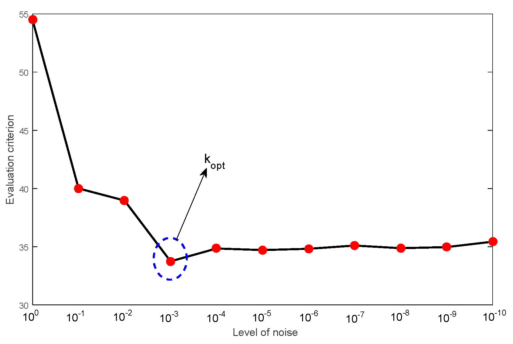
Decompose the PV power output into the IMFs with physical meaning with the improved CEEMDAN (ICEEMDAN). Here, the two critical parameters (the ensemble size and amplitude of the added white noise) are determined by introducing the noise level.

(2)

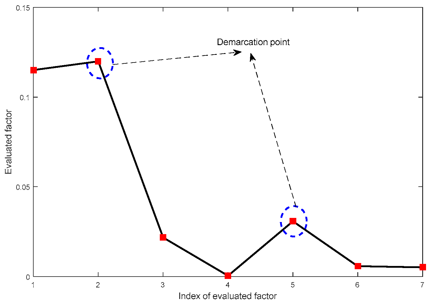
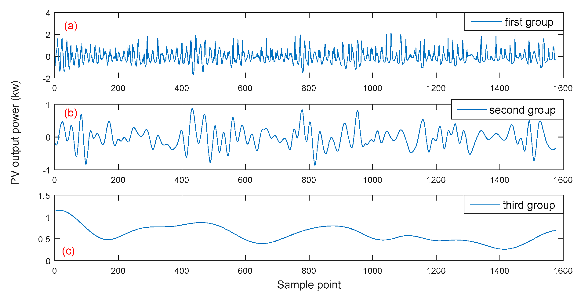
Classify IMFs into the individual feature groups including the most relevant fluctuation components by introducing the comprehensive factor adaptively. It may avoid the drawbacks of threshold determination depending on the empirical method and is an adaptive way.

(3)

Optimize the parameters in the SVM for individual feature groups with the modified PSO (MPSO), and obtain the corresponding sub-forecasting model. The MPSO can enhance the global search ability to make the particle traverse all the space and also local search performance to increase the speed of convergence.

(4)

Reconstruct the sub-forecasting model to obtain the final forecasting model.

(5)

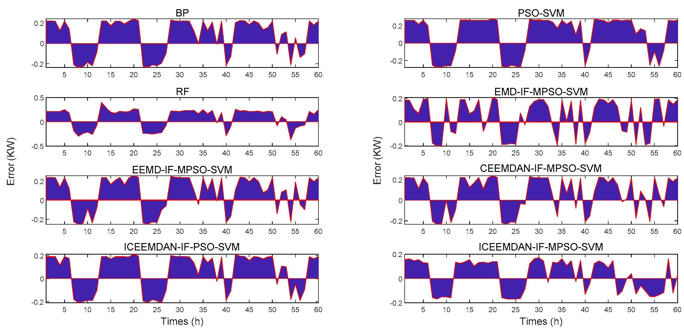
Evaluate the effectiveness of the proposed method (ICEEMDAN-IF-MPSO-SVM), which comes from Step 1 to Step 4.

Figure 1 shows a flowchart of the proposed method.

4. Results and Discussion

This paper uses the PV power output from the UK power network to verify the effectiveness of the proposed method. The time period is the 1 June 2014 to 31 October 2014. Here, only periods between 5 a.m. and 7 a.m. are selected to establish the forecasting model because PV power is almost not generated except during the selected periods. The PV power output is between 0 and 3.5 KW. The data interval is 1 h. The corresponding input variables are six: the time series every day, temperature, wind speed, barometric pressure, rainfall and solar radiation. In addition, because the data including the PV output power and weather conditions are not recorded for each day completely, the final time period is 105 days, and the corresponding data length is 1575. The PV power is plotted in Figure 2.

Here, the data of the first 101 days are set as the training sample. The data of the last 4 days are set as the testing sample. The data length of the testing sample is 60. The autocorrelation function (AF) and partial autocorrelation function (PAF) are used to obtain some insights into whether the PV power output is predictable. The number of lags is set as 60 in the AF and PAF. Figure 3 shows the AF and PAF. It is found that the AF and PAF exhibit significant correlation for most of the numbers of lag. The AF and PAF show obvious periodicity. Especially, the correlation, which belongs to the number of lags at the data point 60, is more than two standard deviations away from 0. This situation, for which the PV power of the first 101 days is used as the training data to predict the PV power of the residue 4 days, is feasible.

Next, the parameter optimization method in Section 3.1 is used to determine the critical parameters of CEEMDAN (the amplitude of the added white noise, NA_opt). Here, the noise level is set from 10⁰ to 10⁻¹⁰, with the step 10⁻¹. The determined index of the noise level is plotted in Figure 4. The findings are that the determination index is the smallest at the noise level of 10⁻³. Thus, the optimal critical parameters are two trails (ensemble size) and ${10}^{-3}\sigma$ (the amplitude of the added white noise), respectively. The $\sigma$ means the standard deviation of the PV power output.

To prove the decomposition effectiveness, the improved CEEMDAN (ICEEMDAN) is used to decompose the PV power output. Meanwhile, the decomposition result is also used to compare that under noise levels of 10⁰, 10⁻¹ and 10⁻². This is shown in Figure 5.

The findings are that the decomposition numbers are 13, 12, 10 and 9 under the noise levels of 10⁰, 10⁻¹, 10⁻² and 10⁻³, respectively. The decomposition number with the proposed method is the smallest. This indicates that the proposed method (ICEEMDAN) can overcome the spurious mode. It also proves that the proposed method can be more suitable for decomposing the PV power output. In the decomposition results under the other noise levels, because the amplitude of the added white noise is relatively large, the white noise is difficult to eliminate. It follows that the interaction of white noise and PV power output introduces a spurious mode (no real physical meaning) and puts the added noise in the IMFs. Finally, the forecasting model is influenced due to the spurious mode and extra noise.

Next, the decomposition IMFs are combined into identified IMFs (IIMFs) according to the equation in Section 3.2. The IIMFs are plotted in Figure 6. The findings are that the waveform characteristics for IIMF1 to IIMF9 are more obvious than those in Figure 5. It is more effective to identify the related modes and classify the IMFs into corresponding feature groups. The findings are that the first feature group should combine IMF1 to IMF3, and the second feature group is from IMF4 to IMF6, as well as the last group being from IMF7 to IMF9.

Here, to prove the effectiveness of the proposed method, the adaptive identified method (IF) in Section 3.2 is used to distinguish the IIMFs. The identified results are plotted in Figure 7. The findings are that the local maxima are the second index and fifth index of the IIMF. It means that the two local maxima divide the IMFs into three groups. According to Equation (22), IMF1 to IMF3, and IMF4 to IMF6, as well as IMF7 to IMF9, are combined into single groups, respectively. This is shown in

Table 2. Combination details with proposed method.

Group Order	First Group	Second Group	Three Group
Combined IMFs	IMF1 + IMF2 + IMF3	IMF4 + IMF5 + IMF6	IMF7 + IMF8 + IMF9

. It proves that the proposed method can classify the related IMFs into corresponding groups effectively. The combined IMFs are plotted in Figure 8. The Figure 8a plots the combined result from IMF1 to IMF3, and the Figure 8b plots the combined result from IMF4 to IMF6, and the Figure 8c plots the combined result from IMF7 to IMF9.

The proposed method is used to forecast the three groups’ PV power output in Figure 8. The modified PSO (MPSO) in Section 3.3 is used to optimize the hyper-parameters in the SVM.

Table 3. Parameter settings in SVM and MPSO.

Order	Name	Value	Order	Name	Value
1	Maximum iteration number	100	6	Iteration number $t_1$	45
2	Start weight	0.9	7	Iteration number $t_2$	90
3	End weight	0.4	8	Parameter C range	0–100
4	Slope $a_1$	−10−4	9	Parameter $\gamma$ range	0–100
5	Slope $a_2$	−10−5	10	Population number	20

indicates the parameter settings in the SVM and MPSO.

Figure 9 shows the comparison of the modified and traditional inertial weight. The findings are that the modified inertial weight has a relatively big weight value in the early stage and small value in the late stage, obviously. They indicate that the modified inertial weight can enhance the global search ability to make the particle traverse all the space and also local search performance to increase the convergence speed.

The SVM is used to forecast the sample of data (combined IMFs in Figure 8). The MPSO is used to optimize the parameters of the SVM in Table 3. The forecasting results are plotted in Figure 10, Figure 11 and Figure 12, respectively. Meanwhile, the error (as shown in Equation (33)), which is the difference between the forecasting result and original series, is used to compare the forecasting effectiveness for each hour’s PV power output.

$$error=x_i-y_{i}i=1,\dots ,N$$

(33)

where $x_i$ refers to the forecasting PV power output, $y_i$ refers to the tested PV power output, and $N$ refers to the number of tested samples.

The error is also plotted in Figure 10, Figure 11 and Figure 12, respectively. The findings are that the forecasting results are all almost consistent with the original tested series of the three groups’ PV power output. For the first group’s PV power output, the forecasting error for the high-frequency component is bigger than that in the low-frequency components (the second group and the third group). The forecasting effectiveness is the best for the third group’s PV power output. Furthermore, it also illustrates the effectiveness of the proposed method; when the different fluctuation components are separated into a single group adaptively, the fluctuation is weaker than in the original series; the forecasting accuracy for each group is better than that for the original series. The final forecasting accuracy from reconstructing the forecasting result of each group should also be better than that for the original series.

The final forecasting result can be obtained by reconstructing the result for each group. Meanwhile, the proposed method (ICEEMDAN-IF-MPSO-SVM) is also compared with ICEEMDAN-IF-PSO-SVM, EEMD-IF-MPSO-SVM, CEEMDAN-IF-MPSO-SVM, EMD-IF-MPSO-SVM, PSO-SVM, back propagation neural network (BP) and random forest (RF) in [42] (as shown in Figure 13a). The MRE, RMSE and R² are used to evaluate the forecasting effectiveness for each forecasting method, respectively.

Table 4. Compared results for the different forecasting methods.

Model	MRE	RMSE	R2
BP	0.3764	0.1919	0.9279
PSO-SVM	0.4817	0.2417	0.8856
RF	0.4194	0.2157	0.9089
EMD-IF-MPSO-SVM	0.3076	0.1596	0.9501
EEMD-IF-MPSO-SVM	0.3829	0.1984	0.9299
CEEMDAN-IF-MPSO-SVM	0.3422	0.1813	0.9356
ICEEMDAN-IF-PSO-SVM	0.3453	0.1741	0.9406
ICEEMDAN-IF-MPSO-SVM	0.2607	0.1329	0.9654

shows the compared results. The findings are that the MRE and RMSE of the proposed method are the smallest among those of all the methods, and the corresponding R² is the biggest. It indicates that the forecasting effectiveness of the proposed method outperforms the other forecasting methods. Additionally, the findings in Figure 13b,c show that the forecasting accuracy for a high amplitude in PV output is better than that for low amplitude.

In addition, the forecasting error for each hour is also plotted in Figure 14. The method of error estimation is same as that in Equation (33). The findings are that the error for the proposed method (ICEEMDAN-IF-MPSO-SVM) is the smallest among all the methods. Furthermore, they also prove that the proposed method is more suitable for forecasting the PV power output.

In addition, the correlation between the forecasting results for the PV power output and the corresponding tested data is also analyzed to evaluate the forecasting effectiveness. Figure 15 plots the correlation. The findings are that the correlation is 0.9910. The forecasting effectiveness has higher accuracy for a high PV power output than that for a low PV power output. Furthermore, this also proves that the proposed method has better forecasting effectiveness.

5. Conclusions

This paper proposes a novel hybrid method for forecasting PV power output. The following conclusions are drawn:

(1)

The ICEEMDAN method is introduced to decompose the PV power output into IMFs with physical meaning. The two critical parameters, which include the ensemble size (EN) and amplitude of the added white noise (NA), can be determined by setting the ensemble size as two trails and introducing the noise level. This method can avoid the interference of a spurious mode for the forecasting of PV power output.

(2)

The adaptive identified method of the relative mode is proposed to classify the IMFs into the corresponding feature groups. The method can separate the complex fluctuating components in PV power output into single components to enhance the forecasting accuracy.

(3)

The modified PSO (MSPO) is proposed to optimize the hyper-parameters in the SVM. The MPSO applies the piecewise inertial weight to enhance the global search ability to make the particle traverse all the space and also local search performance to increase the convergence speed.

Finally, the forecasting result for each group is reconstructed to obtain the desired result. By comparison with the other typical methods, the results indicate that the proposed method is more suitable for forecasting PV power output.

References

1. Kundur, P. Sustainable electric power systems in the 21st century: Requirements, challenges and the role of new technologies. In Proceedings of the IEEE Power Engineering Society General Meeting, Denver, CO, USA, 6–10 June 2004. [Google Scholar]
2. Moro, A.; Holzer, A. A Framework to Predict Consumption Sustainability Levels of Individuals. Sustainability 2020, 12, 1423. [Google Scholar] [CrossRef] [Green Version]
3. Ariyaratna, P.; Muttaqi, K.M.; Sutanto, D. A novel control strategy to mitigate slow and fast fluctuations of the voltage profile at common coupling Point of rooftop solar PV unit with an integrated hybrid energy storage system. J. Energy Storage 2018, 20, 409–417. [Google Scholar] [CrossRef]
4. Huang, C.-J.; Kuo, P.-H. Multiple-Input Deep Convolutional Neural Network Model for Short-Term Photovoltaic Power Forecasting. IEEE Access 2019, 7, 74822–74834. [Google Scholar] [CrossRef]
5. Das, U.K.; Tey, K.S.; Seyedmahmoudian, M.; Idris, M.Y.I.; Mekhilef, S.; Horan, B.; Stojcevski, A. SVR-Based Model to Forecast PV Power Generation under Different Weather Conditions. Energies 2017, 10, 876. [Google Scholar] [CrossRef]
6. Xu, D.; Kang, L.; Chang, L.; Chang, L.; Cao, B. Optimal sizing of standalone hybrid wind/PV power systems using genetic algorithms. In Proceedings of the Canadian Conference on Electrical and Computer Engineering, Saskatoon, SK, Canada, 1–4 May 2005; pp. 1722–1725. [Google Scholar]
7. De Gooijer, J.G.; Hyndman, R.J. 25 years of time series forecasting. Int. J. Forecast. 2006, 22, 443–473. [Google Scholar] [CrossRef] [Green Version]
8. Kim, J.; Jun, S.; Jang, D.; Park, S. Sustainable Technology Analysis of Artificial Intelligence Using Bayesian and Social Network Models. Sustainability 2018, 10, 115. [Google Scholar] [CrossRef] [Green Version]
9. Chui, K.T.; Lytras, M.; Visvizi, A. Energy Sustainability in Smart Cities: Artificial Intelligence, Smart Monitoring, and Optimization of Energy Consumption. Energies 2018, 11, 2869. [Google Scholar] [CrossRef] [Green Version]
10. Sodhro, A.H.; Pirbhulal, S.; De Albuquerque, V.H.C. Artificial Intelligence-Driven Mechanism for Edge Computing-Based Industrial Applications. IEEE Trans. Ind. Inform. 2019, 15, 4235–4243. [Google Scholar] [CrossRef]
11. Chow, S.K.; Lee, E.W.; Li, D.H. Short-term prediction of photovoltaic energy generation by intelligent approach. Energy Build. 2012, 55, 660–667. [Google Scholar] [CrossRef]
12. Jumaat, S.A.B.; Crocker, F.; Wahab, M.H.A.; Radzi, N.H.B.M. Investigate the photovoltaic (PV) module performance using Artificial Neural Network (ANN). In Proceedings of the 2016 IEEE Conference on Open Systems (ICOS), Langkawi, Malaysia, 10–12 October 2016; pp. 59–64. [Google Scholar]
13. Ahmed, R.; Sreeram, V.; Mishra, Y.; Arif, M. A review and evaluation of the state-of-the-art in PV solar power forecasting: Techniques and optimization. Renew. Sustain. Energy Rev. 2020, 124, 109792. [Google Scholar] [CrossRef]
14. Zendehboudi, A. Implementation of GA-LSSVM modelling approach for estimating the performance of solid desiccant wheels. Energy Convers. Manag. 2016, 127, 245–255. [Google Scholar] [CrossRef]
15. Fayazi, A.; Arabloo, M.; Shokrollahi, A.; Zargari, M.H.; Ghazanfari, M.H. State-of-the-Art Least Square Support Vector Machine Application for Accurate Determination of Natural Gas Viscosity. Ind. Eng. Chem. Res. 2013, 53, 945–958. [Google Scholar] [CrossRef]
16. Wang, F.; Li, K.; Wang, X.; Jiang, L.; Ren, J.; Mi, Z.; Shafie-Khah, M.; Catalao, J.P.S. A Distributed PV System Capacity Estimation Approach Based on Support Vector Machine with Customer Net Load Curve Features. Energies 2018, 11, 1750. [Google Scholar] [CrossRef] [Green Version]
17. Niu, D.; Dai, S. A Short-Term Load Forecasting Model with a Modified Particle Swarm Optimization Algorithm and Least Squares Support Vector Machine Based on the Denoising Method of Empirical Mode Decomposition and Grey Relational Analysis. Energies 2017, 10, 408. [Google Scholar] [CrossRef] [Green Version]
18. Pourbasheer, E.; Riahi, S.; Ganjali, M.R.; Norouzi, P. Application of genetic algorithm-support vector machine (GA-SVM) for prediction of BK-channels activity. Eur. J. Med. Chem. 2009, 44, 5023–5028. [Google Scholar] [CrossRef]
19. Chen, P.; Yuan, L.; He, Y.; Luo, S. An improved SVM classifier based on double chains quantum genetic algorithm and its application in analogue circuit diagnosis. Neurocomputing 2016, 211, 202–211. [Google Scholar] [CrossRef]
20. Duan, P.; Xie, K.; Guo, T.; Huang, X. Short-Term Load Forecasting for Electric Power Systems Using the PSO-SVR and FCM Clustering Techniques. Energies 2011, 4, 173–184. [Google Scholar] [CrossRef] [Green Version]
21. Shi, Y.; Eberhart, R. A modified particle swarm optimizer. In Proceedings of the 1998 IEEE international conference on evolutionary computation proceedings. IEEE world congress on computational intelligence (Cat. No. 98TH8360), Anchorage, AK, USA, 4–9 May 1998; pp. 69–73. [Google Scholar]
22. Bansal, J.C.; Singh, P.K.; Saraswat, M.; Verma, A.; Jadon, S.S.; Abraham, A. Inertia weight strategies in particle swarm optimization. In Proceedings of the 2011 Third World Congress on Nature and Biologically Inspired Computing, Salamanca, Spain, 19–21 October 2011; pp. 633–640. [Google Scholar]
23. Ali, M.; Prasad, R.; Xiang, Y.; Deo, R.C. Near real-time significant wave height forecasting with hybridized multiple linear regression algorithms. Renew. Sustain. Energy Rev. 2020, 132, 110003. [Google Scholar] [CrossRef]
24. Abedinia, O.; Amjady, N.; Ghadimi, N. Solar energy forecasting based on hybrid neural network and improved metaheuristic algorithm. Comput. Intell. 2017, 34, 241–260. [Google Scholar] [CrossRef]
25. Yang, Y.; Dong, L. Short-term PV generation system direct power prediction model on wavelet neural network and weather type clustering. In Proceedings of the 2013 5th International Conference on Intelligent Human-Machine Systems and Cybernetics, Hangzhou, China, 26–27 August 2013; Volume 1, pp. 207–211. [Google Scholar]
26. Zhang, P.; Takano, H.; Murata, J. Daily solar radiation prediction based on wavelet analysis. In Proceedings of the SICE Annual Conference 2011, Tokyo, Japan, 13–18 September 2011; pp. 12–717. [Google Scholar]
27. Li, F.-F.; Wang, S.-Y.; Wei, J. Long term rolling prediction model for solar radiation combining empirical mode decomposition (EMD) and artificial neural network (ANN) techniques. J. Renew. Sustain. Energy 2018, 10, 013704. [Google Scholar] [CrossRef]
28. Nayak, N.; Pani, A.K. Short term PV power forecasting using empirical mode decomposition based orthogonal extreme learning machine technique. Indian J. Public Health Res. Dev. 2018, 9, 2170. [Google Scholar] [CrossRef]
29. Abedinia, O.; Lotfi, M.; Bagheri, M.; Sobhani, B.; Shafie-Khah, M.; Catalao, J.P.S. Improved EMD-Based Complex Prediction Model for Wind Power Forecasting. IEEE Trans. Sustain. Energy 2020, 99, 1. [Google Scholar] [CrossRef]
30. Abedinia, O.; Raisz, D.; Amjady, N. Effective prediction model for Hungarian small-scale solar power output. IET Renew. Power Gener. 2017, 11, 1648–1658. [Google Scholar] [CrossRef]
31. Prasad, R.; Ali, M.; Kwan, P.; Khan, H. Designing a multi-stage multivariate empirical mode decomposition coupled with ant colony optimization and random forest model to forecast monthly solar radiation. Appl. Energy 2019, 236, 778–792. [Google Scholar] [CrossRef]
32. Ali, M.; Deo, R.C.; Maraseni, T.; Downs, N.J. Improving SPI-derived drought forecasts incorporating synoptic-scale climate indices in multi-phase multivariate empirical mode decomposition model hybridized with simulated annealing and kernel ridge regression algorithms. J. Hydrol. 2019, 576, 164–184. [Google Scholar] [CrossRef]
33. Prasad, R.; Ali, M.; Xiang, Y.; Khan, H. A double decomposition-based modelling approach to forecast weekly solar radiation. Renew. Energy 2020, 152, 9–22. [Google Scholar] [CrossRef]
34. Wu, Z.; Huang, N.E. Ensemble empirical mode decomposition: A noise-assisted data analysis method. Adv. Adapt. Data Anal. 2009, 1, 1–41. [Google Scholar] [CrossRef]
35. Torres, M.E.; Colominas, M.A.; Schlotthauer, G.; Flandrin, P. A complete ensemble empirical mode decomposition with adaptive noise. In Proceedings of the Acoustics, Speech and Signal Processing (ICASSP), 2011 IEEE International Conference on IEEE, Prague, Czech Republic, 22–27 May 2011; pp. 4144–4147. [Google Scholar]
36. Ali, M.; Prasad, R. Significant wave height forecasting via an extreme learning machine model integrated with improved complete ensemble empirical mode decomposition. Renew. Sustain. Energy Rev. 2019, 104, 281–295. [Google Scholar] [CrossRef]
37. Ali, M.; Prasad, R.; Xiang, Y.; Yaseen, Z.M. Complete ensemble empirical mode decomposition hybridized with random forest and kernel ridge regression model for monthly rainfall forecasts. J. Hydrol. 2020, 584, 124647. [Google Scholar] [CrossRef]
38. Zhang, J.; Yan, R.; Gao, R.X.; Feng, Z. Performance enhancement of ensemble empirical mode decomposition. Mech. Syst. Signal Process. 2010, 24, 2104–2123. [Google Scholar] [CrossRef]
39. Niazy, R.K.; Beckmann, C.F.; Brady, J.M.; Smith, S.M. Performance Evaluation of Ensemble Empirical Mode Decomposition. Adv. Adapt. Data Anal. 2009, 1, 231–242. [Google Scholar] [CrossRef]
40. Wang, H.; Sun, J.; Wang, W.-J. Photovoltaic Power Forecasting Based on EEMD and a Variable-Weight Combination Forecasting Model. Sustainability 2018, 10, 2627. [Google Scholar] [CrossRef] [Green Version]
41. Liu, Z.; Sun, W.; Zeng, J. A new short-term load forecasting method of power system based on EEMD and SS-PSO. Neural Comput. Appl. 2013, 24, 973–983. [Google Scholar] [CrossRef]
42. Oneto, L.; Laureri, F.; Robba, M.; Delfino, F.; Anguita, D. Data-Driven Photovoltaic Power Production Nowcasting and Forecasting for Polygeneration Microgrids. IEEE Syst. J. 2017, 12, 2842–2853. [Google Scholar] [CrossRef]
Figure 1. Flowchart of proposed method.
Symmetry 12 01777 g001
Figure 2. PV power output.
Symmetry 12 01777 g002
Figure 3. Analysis of autocorrelation function (AF) and partial autocorrelation function (PAF) of PV power.
Symmetry 12 01777 g003
Figure 4. Determination index for critical parameters.
Symmetry 12 01777 g004
Figure 5. Decomposition comparison of PV power output.
Symmetry 12 01777 g005
Figure 6. Combined IMF under optimal decomposition.
Symmetry 12 01777 g006
Figure 7. Identification of demarcation point between IMFs.
Symmetry 12 01777 g007
Figure 8. Combined IMF with proposed method. (a) plots the combined result from IMF1 to IMF3, and the (b) plots the combined result from IMF4 to IMF6, and the (c) plots the combined result from IMF7 to IMF9.
Symmetry 12 01777 g008
Figure 9. Comparison of modified and traditional inertial weight.
Symmetry 12 01777 g009
Figure 10. Forecasting result and error for the first group.
Symmetry 12 01777 g010
Figure 11. Forecasting result and error for the second group.
Symmetry 12 01777 g011
Figure 12. Forecasting result and error for the third group.
Symmetry 12 01777 g012
Figure 13. Comparison of different forecasting methods for PV output.
Symmetry 12 01777 g013
Figure 14. Comparison of forecasting errors for different methods.
Symmetry 12 01777 g014
Figure 15. Correlation between forecasting results and original tested series.
Symmetry 12 01777 g015