Global Stabilization of a Reaction Wheel Pendulum: A Discrete-Inverse Optimal Formulation Approach via A Control Lyapunov Function

Abstract

This paper deals with the global stabilization of the reaction wheel pendulum (RWP) in the discrete-time domain. The discrete-inverse optimal control approach via a control Lyapunov function (CLF) is employed to make the stabilization task. The main advantages of using this control methodology can be summarized as follows: (i) it guarantees exponential stability in closed-loop operation, and (ii) the inverse control law is optimal since it minimizes the cost functional of the system. Numerical simulations demonstrate that the RWP is stabilized with the discrete-inverse optimal control approach via a CLF with different settling times as a function of the control gains. Furthermore, parametric uncertainties and comparisons with nonlinear controllers such as passivity-based and Lyapunov-based approaches developed in the continuous-time domain have demonstrated the superiority of the proposed discrete control approach. All of these simulations have been implemented in the MATLAB software.

1. Introduction

Dynamics of nonlinear systems is a central concern in science, engineering, and mechanical problems. In order to analyze them, test prototypes represent a powerful strategy [1]. This is because their nonlinear dynamics allow getting a better grasp of the phenomena and physical behavior of several industries and equipment applications including: robotic systems, aerospace systems, marine vehicles [2,3]. There exist multiple versions of the classic models of the pendulum, among which the most known are the reaction wheel pendulum (RWP), the pendulum on a cart with linear displacement, the Furuta pendulum with a rotating base, and also these with two and three bars, among others. This study considers the well-know educative RWP dynamical system.

The RWP is an inverted pendulum balanced by a flywheel, i.e., an actuated rotating reaction wheel. It exhibits important challenges in the field of control theory including robustness, stabilization, and nonlinearities. These features combined make it an attractive and adequate system for performing research and high-level education. Various engineering problems can be modeled similarly as inverted pendulum, including rocket launch and human-powered vehicles.

In the literature, the problem of control in RWP has been addressed with both linear and non-linear techniques as well as artificial intelligent methods. These can be found mainly as: control Lyapunov functions [4], passivity-based control [5], proportional-integral controllers [6], fuzzy logic [7], feedback linearization [8], and deep neural networks [9].

The below-mentioned items represent the key aspects that make this approach different from similar works:

✓

Global stabilization of the discrete version of the RWP dynamic model system via control Lyapunov functions with global exponential convergence and optimality properties.

✓

Robustness performance against parametric uncertainties while preserving asymptotic convergence properties.

✓

The comparison of the proposed discrete-inverse optimal controllers via control Lyapunov functions with the discrete versions of the passivity-based and Lyapunov-based controllers (from the continuous domain) demonstrating superior performances regarding stabilization of the RWP system with minimum settling times.

After a thorough literature review regarding the different approaches to the RWP dynamical system modeling and control, we identified a niche to occupy. Despite the wide variety of methods presented to date, strategies based on discrete-inverse optimal control are scarcely applied to model this sort of system [10,11,12]. Therefore, it stands for the research gap this article tries to occupy.

To design a discrete inverse optimal controller via a CLF, it is required to obtain a discrete version of the dynamic model of the RWP system [13]. Here, we use the forward difference method to obtain this discrete equivalent. In addition, it is worth mentioning that the proposed controller is based on the discrete control theory presented in [11]. It is mandatory to have the discrete version of the studied plant for developing any simulation using the approach here proposed.

Regarding the design of the discrete inverse optimal controller, it is important to highlight that: (i) it is based on the discrete version of the classical optimal control theory that works with the discrete-time Hamilton–Jacobi–Bellman (DT-HJB) equivalent [12], and (ii) the solution of this partial differential equation is referenced in the literature as the function value associated with a functional cost for some discrete dynamic system [14]. Here, we use the DT-HJB solutions, which implies that this control law is optimal for the reaction wheel pendulum [11].

The remainder of this study is organized as follows: Section 2 presents the continuous dynamical formulation of the RWP and its discrete version using the backward difference method with discretization time $T_s$. Section 3 presents the general theory about discrete-inverse optimal control designs via control Lyapunov functions; also, it is presented the proof of the exponential stabilization capabilities and optimality properties. Section 4 presents all the numerical validations including parametric uncertainties, variations in the control gains, and comparisons with nonlinear classical methodologies developed in the continuous domain. Section 5 presents the main conclusions derived from this research and some guidelines for possible future works.

2. Dynamical Modeling of the Reaction Wheel Pendulum

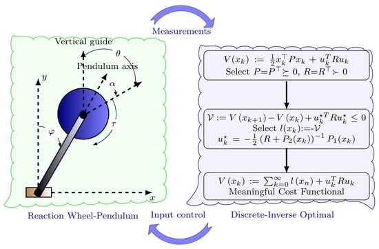
One of the most classical dynamical systems used in education is the RWP, since it allows verifying multiple linear and nonlinear control strategies that deal with nonlinearities caused by trigonometric relationships between the system variables [10]. The dynamical structure of the RWP system emerges in different applications such as transportation systems, bridge crane models, synchronous machines used in power systems, among others. A schematic bi-dimensional representation of the RWP system is depicted in Figure 1, where the main physical variables have been reported [4,15].

In the physical representation of the RWP system presented in Figure 1, we can observe the following variables: the pendulum angle $\phi$ (from the vertical axis) and the angle $\alpha$ between the pendulum and wheel, which are measured with sensors located at each of the axes of rotation. In addition, this system has a motor coupled to the opposite end of the pivot, acting on an inertia wheel, which allows controlling oscillations on it to the reaction torque $\tau$. The dynamic model of this system is derived as follows in the continuous-time domain.

2.1. Dynamical Model in the Continuous Domain

The first step in obtaining a discrete dynamical formulation of the RWP system corresponds to define its continuous formulation. For doing so, let us define an auxiliary variable named $\theta =\phi +\alpha$. With this definition, the dynamical model of the RWP system is defined by (1) as recommended in [15].

$$\begin{array}{c}\hfill \begin{array}{cc}\hfill \ddot{\phi }& =asin\left(\phi \right)-bu,\hfill \\ \hfill \ddot{\theta }& =cu,\hfill \end{array}\end{array}$$

(1)

where a, b, and c represent positive constants related to the physical parameters of the system, $\phi$ defines the angular position of the pendulum measured from the vertical axis, and $\theta$ is the relative angle of the reaction wheel measured from the same vertical axis.

The control input u couple the electric DC motor variables with the reaction wheel movement variables. Note that the control input represents the amount of voltage applied to the DC motor, which is traduced by the current flow into it to a mechanical torque applied directly to the reaction wheel [8]. This torque moves the wheel, which in turn makes the pendulum bar moves from the initial point to the desired upright position [13]. In addition, due to the structure of the nonlinear dynamical model (1) the behavior of the variable $\theta$ is wholly defined as the double integral of the control input u. In addition, this variable does not affect the angular position of the pendulum directly since both Equations in (1) are uncoupled. This situation allows ensuring that the dynamics of the angular speed $\dot{\theta }$ and the angular position of the reaction wheel, i.e., $\theta$ can be wholly known as follows:

$$\begin{array}{c}\hfill \dot{\theta }=c{\int }_0^{t}u\left(\tau \right)d\tau ,\\ \hfill \theta =c{\int }_0^{\zeta }\left({\int }_0^{t}u\left(\tau \right)d\tau \right)dz.\end{array}$$

Observe that if the control input is of class one, i.e., $u\in {\mathcal{C}}^1$, and it is upper and lower bounded, then the angular speed of the reaction wheel, i.e., $\dot{\theta }$, will tend to zero when the angular position of the pendulum and its angular speed reach the equilibrium point.

Remark 1.

Note when the angular speed of the reaction wheel goes to zero, this implies that the angular position of this wheel, i.e., θ, reaches a constant value, which corresponds to its equilibrium point, since from (1), we know that ${\dot{\theta }}^{\star }=0$ for $u^{\star }$, and ${\theta }^{\star }=k$, being k a real constant. It is worth mentioning that $x^{\star }$ must be understood as the equilibrium point of the state variable x.

From the transformation of the dynamical system (1) to a state-space representation, we define the following state variables: $x_1=\phi$ and $x_2={\dot{x}}_1$. Now, if these are substituted in (1), then, the following second-order dynamical model yields:

$$\begin{array}{c}\hfill \begin{array}{cc}\hfill {\dot{x}}_1& =x_2,\hfill \\ \hfill {\dot{x}}_2& =asin\left(x_1\right)-bu.\hfill \end{array}\end{array}$$

(2)

Remark 2.

The RWP system defined in (2) has two main equilibrium points, which have infinite repetitions. These two main points are P${}_1\left(x_1^{\star },x_2^{\star }\right)=$ P${}_1\left(0,0\right)$ and P${}_2\left(x_1^{\star },x_2^{\star }\right)=$ P${}_1\left(\pi ,0\right)$; which are cyclical each $2k\pi$, being k a integer number. However, the main interest of controlling an RWP is to maintain its upright position from any initial position, i.e., to regulate all the state variables over P${}_1$.

2.2. Dynamical Model in the Discrete Domain

The representation of the RWP system in the discrete domain is reached by using the classical forward difference, which allows knowing the next step, i.e., $x_{k+1}$, as a function of the current information of the system [16], i.e., $x_k$. This forward difference takes the following form [17,18]:

$$\begin{array}{c}\hfill \frac{d}{dt}x=\frac{x_{k+1}-x_k}{T_s},\end{array}$$

(3)

where $T_s$ represent the discretization time.

Note that if we apply the discretization defined in (3) on (2), then, we reach the following discrete model for the RWP system:

$$\begin{array}{c}\hfill \begin{array}{cc}\hfill x_{1_{k+1}}& =T_s{x}_{2_k}+x_{1_k},\hfill \\ \hfill x_{2_{k+1}}& =T_{s}asin\left(x_{1_k}\right)+x_{2_k}-T_{s}b{u}_k.\hfill \end{array}\end{array}$$

(4)

For the sake of compactness, the discrete dynamical model of the RWP model defined in (4) is rewritten as follows:

$$\begin{array}{c}\hfill x_{k+1}=f\left(x_k\right)+g\left(x_k\right)u_k,\end{array}$$

(5)

where $f\left(x_k\right)\in {\mathbb{R}}^{n\times 1}$ corresponds to a vector of nonlinear functions of the state variables and $g\left(x_k\right)\in {\mathbb{R}}^{n\times m}$ is known as the input matrix, $x_k\in {\mathbb{R}}^{n\times 1}$ is the vector of all the state variables, and $u_k\in {\mathbb{R}}^{m\times 1}$ in an m-dimensional vector that contains all the control inputs. It is worth mentioning that in the case of the RWP system $n=2$ and $m=1$, which implies that functions in (5) take the following form:

$$\begin{array}{c}\hfill f\left(x_k\right)=\left[\begin{array}{c}{T}_s{x}_{2_k}+x_{1_k}\\ T_{s}asin\left(x_{1_k}\right)+x_{2_k}\end{array}\right],g\left(x_k\right)=\left[\begin{array}{c}0\\ -T_{s}b\end{array}\right].\end{array}$$

(6)

To develop a discrete-inverse optimal controller via control Lyapunov functions, the compact structure of the RWP system defined in (5) is considered as it will presented in the next section.

3. Discrete-Inverse Optimal Formulation via CLF

Using Lyapunov functions in control theory allows developing robust methodologies for controlling physical systems in continuous or discrete representations. The main advantage of using this approach is the global asymptotic stability performance under well-defined operative conditions of the system [11]. Here, we employ the discrete-inverse optimal control theory to develop a nonlinear controller applicable to the RWP system with optimal and asymptotic properties [19].

Definition 1.

(Inverse optimal control law (taken from [11])). The following control law

$$\begin{array}{c}\hfill u_k^{\star }=-\frac{1}{2}{R}^{-1}g{\left(x_k\right)}^T\frac{\partial V\left(x_{k+1}\right)}{\partial x_{k+1}},\end{array}$$

(7)

where $R^{-1}$ is a square $m\times m$ matrix associated with the number of control inputs, and $g{\left(x_k\right)}^T$ is the transpose operation applied on the input matrix $g\left(x_k\right)$ is said inverse optimal if:

(i) 

it allows achieving the global exponential stability of the equilibrium point $x_k=0$ for the discrete system (5), and

(ii) 

it minimizes a cost functional defined as (8)

$$\begin{array}{c}\hfill V\left(x_k\right)=\sum _{n=k}^{\infty }l\left(x_n\right)+u_n^{T}R{u}_n,\end{array}$$

(8)

with $l\left(x_k\right):=-\mathcal{V}$, being

$$\begin{array}{c}\hfill \mathcal{V}:=V\left(x_{k+1}\right)-V\left(x_k\right)+u_k^{\star T}R{u}_k^{\star }.\end{array}$$

(9)

Note that Definition 1 is based on the complete knowledge of the function $V\left(x_k\right)$. Here, we employ a classical hyperparaboloid CLF with the structure presented in (10).

$$\begin{array}{c}\hfill V\left(x_k\right)=\frac{1}{2}{x}_k^{T}P{x}_k,\end{array}$$

(10)

where P is a symmetric positive definite matrix with appropriate dimensions.

To obtain a general inverse optimal control law as defined in (7), we can substitute (10) into it, which yields:

$$\begin{array}{cc}\hfill u_k^{\star }& =-\frac{1}{2}{R}^{-1}g{\left(x_k\right)}^T\frac{\partial V\left(x_{k+1}\right)}{\partial x_{k+1}}\hfill \\ \hfill & =-\frac{1}{2}{R}^{-1}g{\left(x_k\right)}^{T}P{x}_{k+1}\hfill \\ \hfill & =-\frac{1}{2}{R}^{-1}g{\left(x_k\right)}^T\left(Pf\left(x_k\right)+Pg\left(x_k\right)u_k^{\star }\right)\hfill \\ \hfill \left(I+\frac{1}{2}{R}^{-1}g{\left(x_k\right)}^{T}Pg\left(x_k\right)\right)u_k^{\star }& =-\frac{1}{2}{R}^{-1}g{\left(x_k\right)}^{T}Pf\left(x_k\right),\hfill \end{array}$$

(11)

where I is an identity matrix with appropriate dimensions.

Now, if we define $P_1\left(x_k\right)=g{\left(x_k\right)}^{T}Pf\left(x_k\right)$ and $P_2\left(x_k\right)=g{\left(x_k\right)}^{T}Pg\left(x_k\right)$, then, Equation (11) generates the following inverse optimal control law:

$$\begin{array}{c}\hfill u_k^{\star }=-\frac{1}{2}{\left(R+P_2\left(x_k\right)\right)}^{-1}{P}_1\left(x_k\right),\end{array}$$

(12)

where both parts of (11) have been pre-multiplied by R.

Remark 3.

The existence of the inverse optimal control law is ensured due to the positive definite and symmetry properties of the $P_2\left(x_k\right)$ matrix, which ensures the existence of the inverse in (12) [11].

3.1. Global Stability Test

The inverse optimal control law (12) guarantees the global stability behavior in the discrete-affine dynamic system (5) if the following inequality constraint is held [11]

$$\begin{array}{c}\hfill V_f\left(x_k\right)-\frac{1}{4}{P}_1^T\left(x_k\right){\left(R+P_2\left(x_k\right)\right)}^{-1}{P}_1\left(x_k\right)-{\lambda }_Q{\left|\left|x_k\right|\right|}^2\le 0,\end{array}$$

(13)

for some $P=P^T>0$, $V_f\left(x_k\right)=V\left(f\left(x_k\right)\right)-V\left(x_k\right)$, being $V\left(f\left(x_k\right)\right)=\frac{1}{2}{f}^T\left(x_k\right)Pf\left(x_k\right)$, and ${\lambda }_Q>0$.

To verify that the condition (13) is required, let us to recur to the definition of $\mathcal{V}$ in (9) where we substitute $\alpha \left(x_k\right)=u_k^{\star }$, which produces:

$$\begin{array}{cc}\hfill \mathcal{V}& =V\left(x_{k+1}\right)-V\left(x_k\right)+{\alpha }^T\left(x_k\right)R\alpha \left(x_k\right)\hfill \\ \hfill & =\frac{f^T\left(x_k\right)Pf\left(x_k\right)+2f^T\left(x_k\right)Pg\left(x_k\right)\alpha \left(x_k\right)}{2}+\frac{{\alpha }^T\left(x_k\right)g^T\left(x_k\right)Pg\left(x_k\right)\alpha \left(x_k\right)-x_k^{T}P{x}_k}{2}\hfill \\ \hfill & +{\alpha }^T\left(x_k\right)R\alpha \left(x_k\right)\hfill \\ \hfill & =V_f\left(x_k\right)-\frac{1}{2}{P}_1^T\left(x_k\right){\left(R+P_2\left(x_k\right)\right)}^{-1}{P}_1^T\left(x_k\right)+\frac{1}{4}{P}_1^T\left(x_k\right){\left(R+P_2\left(x_k\right)\right)}^{-1}{P}_1^T\left(x_k\right)\hfill \\ \hfill & =V_f\left(x_k\right)-\frac{1}{4}{P}_1^T\left(x_k\right){\left(R+P_2\left(x_k\right)\right)}^{-1}{P}_1^T\left(x_k\right).\hfill \end{array}$$

(14)

Note that if P is selected such that $\mathcal{V}<0$, then, the asymptotic stability is ensured around the equilibrium point $x_k=0$. Furthermore, through P, we can achieve a desired negativity amount for the closed-loop function $\mathcal{V}$ in Expression (14). Note that this desired negativity can be satisfied by defining a positive definite matrix Q such that:

$$\begin{array}{cc}\hfill \mathcal{V}& =V_f\left(x_k\right)-\frac{1}{4}{P}_1^T\left(x_k\right){\left(R+P_2\left(x_k\right)\right)}^{-1}{P}_1^T\left(x_k\right)\hfill \\ \hfill & \le -x_k^{T}Q{x}_k\hfill \\ \hfill & \le -{\lambda }_{min}\left(Q\right){\left|\left|x_k\right|\right|}^2=-{\lambda }_Q{\left|\left|x_k\right|\right|}^2,\hfill \end{array}$$

(15)

where $\left|\left|·\right|\right|$ corresponds to any norm, for simplicity it could be Euclidean norm; and ${\lambda }_Q>0$ defines the minimum eigenvalue of the matrix Q; which implies that (15) maintains the condition (13).

Now, if we compare (14) and (15), then,

$$\begin{array}{c}\hfill \mathcal{V}=V\left(x_{k+1}\right)-V\left(x_k\right)+{\alpha }^T\left(x_k\right)R\alpha \left(x_k\right)\le -{\lambda }_Q{\left|\left|x_k\right|\right|}^2\to V\left(x_{k+1}\right)-V\left(x_k\right)\le -{\lambda }_Q{\left|\left|x_k\right|\right|}^2.\end{array}$$

(16)

Remark 4.

Due to $V\left(x_k\right)$ being a radially unbounded function, then, the solution $x_k=0$ of the discrete-affine system (5) with (12) is global exponentially stable according to [19,20].

3.2. Optimality Test

To demonstrate that the discrete-inverse control law $u_k^{\star }$ defined in (7) is optimal, let us consider the function $l\left(x_k\right)$ as follows:

$$\begin{array}{cc}\hfill l\left(x_k\right)& {:=-\mathcal{V}|}_{u_k^{\star }=\alpha \left(x_k\right)}\hfill \\ \hfill & =-V_f\left(x_k\right)+\frac{1}{4}{P}_1^T\left(x_k\right){\left(R+P_2\left(x_k\right)\right)}^{-1}{P}_1\left(x_k\right),\hfill \end{array}$$

(17)

where $V\left(x_k\right)$ is the solution of the DT-HJB equation, i.e.,

$$\begin{array}{c}\hfill l\left(x_k\right)+V^{\star }\left(x_{k+1}\right)-V^{\star }\left(x_k\right)+\frac{1}{4}\frac{\partial V^{\star T}\left(x_{k+1}\right)}{\partial x_{k+1}}g\left(x_k\right)R^{-1}{g}^T\left(x_k\right)\frac{\partial V^{\star }\left(x_{k+1}\right)}{\partial x_{k+1}}=0.\end{array}$$

To obtain the optimal value for the cost functional defined in (8), let us substitute (17) on it as follows:

$$\begin{array}{cc}\hfill V\left(x_k\right)& =\sum _{k=0}^{\infty }l\left(x_n\right)+u_k^{T}R{u}_k\hfill \\ \hfill & =\sum _{k=0}^{\infty }-\mathcal{V}+u_k^{T}R{u}_k\hfill \\ \hfill & =-\sum _{k=0}^{\infty }{V}_f\left(x_k\right)-\frac{1}{4}{P}_1^T\left(x_k\right){\left(R+P_2\left(x_k\right)\right)}^{-1}{P}_1\left(x_k\right)+\sum _{k=0}^{\infty }{u}_k^{T}R{u}_k.\hfill \end{array}$$

(18)

To simplify Expression (18), we recur to an identity matrix with the form $\left(R+P_2\left(x_k\right)\right){\left(R+P_2\left(x_k\right)\right)}^{-1}$, which allows rewriting it as presented below.

$$\begin{array}{cc}\hfill V\left(x_k\right)& =-\sum _{k=0}^{\infty }\left[\begin{array}{c}{V}_f\left(x_k\right)-\frac{1}{2}{P}_1^T\left(x_k\right){\left(R+P_2\left(x_k\right)\right)}^{-1}{P}_1\left(x_k\right)\\ +\frac{1}{4}{P}_1^T\left(x_k\right){\left(R+P_2\left(x_k\right)\right)}^{-1}{P}_2\left(x_k\right){\left(R+P_2\left(x_k\right)\right)}^{-1}{P}_1\left(x_k\right)\\ +\frac{1}{4}{P}_1^T\left(x_k\right){\left(R+P_2\left(x_k\right)\right)}^{-1}R{\left(R+P_2\left(x_k\right)\right)}^{-1}{P}_1\left(x_k\right)\end{array}\right]+\sum _{k=0}^{\infty }{u}_k^{T}R{u}_k,\hfill \end{array}$$

(19)

Now, from (12) we know that $\alpha \left(x_k\right)=-\frac{1}{2}{\left(R+P_2\left(x_k\right)\right)}^{-1}{P}_1\left(x_k\right)$, which implies that (19) can take the following form:

$$\begin{array}{cc}\hfill V\left(x_k\right)& =-\sum _{k=0}^{\infty }\left[\begin{array}{c}{V}_f\left(x_k\right)+P_1^T\left(x_k\right)\alpha \left(x_k\right)+{\alpha }^T\left(x_k\right)P_2\left(x_k\right)\alpha \left(x_k\right)\end{array}\right]+\sum _{k=0}^{\infty }\left[\begin{array}{c}{u}_k^{T}R{u}_k-{\alpha }^T\left(x_k\right)R\alpha \left(x_k\right)\end{array}\right].\hfill \end{array}$$

(20)

Remembering the definitions of $V_f\left(x_k\right)$, $P_1\left(x_k\right)$, and $P_2\left(x_k\right)$, we can simplify (20) as presented below.

$$\begin{array}{c}\hfill V\left(x_k\right)=-\sum _{k=0}^{\infty }\left[\begin{array}{c}V\left(x_{k+1}\right)-V\left(x_k\right)\end{array}\right]+\sum _{k=0}^{\infty }\left[\begin{array}{c}{u}_k^{T}R{u}_k-{\alpha }^T\left(x_k\right)R\alpha \left(x_k\right)\end{array}\right].\end{array}$$

(21)

Note that if the upper bound of the sum is defined as N, then, we obtain from (22) the following result:

$$\begin{array}{c}\hfill V\left(x_k\right)=-\underset{N\to \infty }{lim}\left[\begin{array}{c}V\left(x_N\right)-V\left(x_0\right)\end{array}\right]+\sum _{k=0}^{\infty }\left[\begin{array}{c}{u}_k^{T}R{u}_k-{\alpha }^T\left(x_k\right)R\alpha \left(x_k\right)\end{array}\right].\end{array}$$

(22)

where we can observe that $V\left(x_N\right)\to 0$ when $N\to 0$ due the global exponential convergence presented in the previous section; this implies that Expression (22) can be written as follows:

$$\begin{array}{c}\hfill V\left(x_k\right)=V\left(x_0\right)+\sum _{k=0}^{\infty }\left[\begin{array}{c}{u}_k^{T}R{u}_k-{\alpha }^T\left(x_k\right)R\alpha \left(x_k\right)\end{array}\right].\end{array}$$

(23)

Remark 5.

From (23), it is possible to conclude that the maximum value is reached when $u_k=\alpha \left(x_k\right)$, which implies that the control law (12) is indeed optimal, since it minimizes the cost functional (8), where the optimal solution is:

$$\begin{array}{c}\hfill V^{\star }\left(x_k\right)=V\left(x_0\right),\end{array}$$

for all $x_0$.

4. Numerical Validations

To demonstrate the effectiveness and robustness of the proposed discrete-inverse optimal control design via control Lyapunov functions, we consider that the dynamical model (5) has the following constants: $a=78.4{\left(\frac{\mathrm{rad}}{s}\right)}^2$ and $b=1.08\frac{\mathrm{rad}}{s^2}$, these values were taken from [7]. It is important to mention that as recommended in [21], the magnitude of the control function, i.e., $\left|u_k\right|$, can be at most 10. Note that the control gains inside of the P matrix have been defined using a heuristic search based on multiple simulations as follows:

$$\begin{array}{c}\hfill P=\left[\begin{array}{cc}12\times {10}^8& 32\times {10}^6\\ 32\times {10}^6& 12\times {10}^5\end{array}\right].\end{array}$$

4.1. Evaluation of the Controller for Different Values of the R Gain

The effectiveness of the proposed controller is tested considering the aforementioned parameters; also, the simulation was run for some values of gain R in the interval between $0.50$ and $2.5$ in steps of $0.50$ (this interval is selected based on heuristic evaluations using multiple intervals of analysis. However, these values enclosed most of the possible behaviors reached by the proposed controller when applied to the RWP system.). In this case the initial conditions are $\left(x_{1_0},x_{2_0}\right)=\left(\frac{7\pi }{180},0\right)$. Note that these initial guesses have been selected based on the physical recommendations for the RWP system provided in reference [21], where these can avoid over-saturation events in the control input.

Figure 2 reports the behavior of the angular position of the pendulum bar, its velocity, and the control input. From these results, we can observe that:

✓

The gain R highly influences the behavior of the angular position of the RWP system depicted in Figure 2a, since small values of this allows reaching the desired operational point about in 375 samples, (i.e., 375 ms) (see curves for $R=1$ and $R=10$); however, when this parameter increases then the system exhibits oscillations around the desired point and the settling time is between 400 ms and 700 ms.

✓

The angular speed of the pendulum bar depicted in Figure 2b presents a negative acceleration between the interval from 0 ms to 300 ms. However, when the concave form of the angular position changes to a convex one, this velocity is reduced from its negative maximum to zero. In addition, the figure shows the overpass in the angular position due to the effects produced on this by the R gain.

✓

For small values of the R gain, it is possible to observe two main saturations of the control gain about 10 and $-10$ (see Figure 2). These saturations imply that the motor, coupled with the reaction wheel, is accelerated to its maximum values to reach the desired operative point in minimum settling times. When the R gain increases, it is possible to observe that the second saturation disappears which enlarge the settling times of the state variables, due to the acceleration of the motor is not at its maximums.

Figure 3 presents the phase-portrait of the state variables and the evaluation of the Lyapunov function, which have been normalized with the maximum of the cost functional given by $V\left(x_0\right)=\frac{1}{2}{x}_0^{T}P{x}_0$. From Figure 3, we can observe that: (i) the phase portrait of the state variables show that for all the tested values of the R gain, the system is global exponentially stabilized via discrete-inverse optimal control based on a CLF design (see Figure 3a); and (ii) the Lyapunov function presented in Figure 3b confirms that the selected gains in the control matrix P generate a positive definite matrix, which makes that the Lyapunov function is always positive or zero. Additionally, it is confirmed that for $N=1000$ samples, the final value of this function is zero, which implies that the cost functional is maximum as demonstrated in (23).

4.2. Performance under Parametric Variations

To demonstrate that the proposed discrete-inverse optimal controller via CLF design is efficient under parametric variations, we evaluate variations in the a and b parameters from $50\%$ to $150\%$ of its rate values in steps of $25\%$. In this simulation is assumed that the R gain is settled as 1. Note that in this simulation case, the controller has been settling with the parameters a and b at their nominal values, i.e., $100\%$ of these.

Results in Figure 4 confirm that the proposed discrete-inverse optimal controller allows reaching global asymptotic stability in the angular position of the pendulum bar independent on the parametric variations of the constants a and b. However, for values lower than the $100\%$ of these, the settling time increases, while for values larger than this bound, this time is reduced. This situation is attributable to the multiplication effect that has the gain b regarding the control input, as can be seen in the discrete model (4), which can attenuate or increment the effect of the control input in the closed-loop dynamics of the RWP system.

4.3. Comparison with Nonlinear Controllers

Here, the proposed inverse optimal control via CLF is compared with a nonlinear controller based on a direct Lyapunov control proposed in [4], the structure of this control law is presented below

$$\begin{array}{c}\hfill u_k=\frac{1}{T_{s}b}\left(k_1{x}_{1_k}+k_2{x}_{2_k}+2asin\left(x_{1_k}\right)\right),\end{array}$$

(24)

being $k_1$ and $k_2$ defined as 3500 and 135, respectively. In addition, the proposed inverse optimal control is also compared with a nonlinear passivity-based controller proposed in [5], which has the following control law

$$\begin{array}{c}\hfill u_k=\frac{1}{T_{s}b}\left(-j_1\alpha x_{1_k}+r_2{x}_{2_k}+asin\left(x_{1_k}\right)\right),\end{array}$$

(25)

being $j_1=-1$, $\alpha =3500$ and $r_2=135$, which are selected to make it comparative with the Lyapunov-based design.

It is important to mention that all the three controllers defined in (12), (24), and (25) are based on Lyapunov stability theory, which implies that all of them have global asymptotic stability properties for the closed-loop operation. In addition, it is possible to observe that all of them have a very similar control law, which is composed of linear feedback of the states $x_{1_k}$ and $x_{2_k}$ and the nonlinear effect of the sinusoidal function weighted by a constant [22].

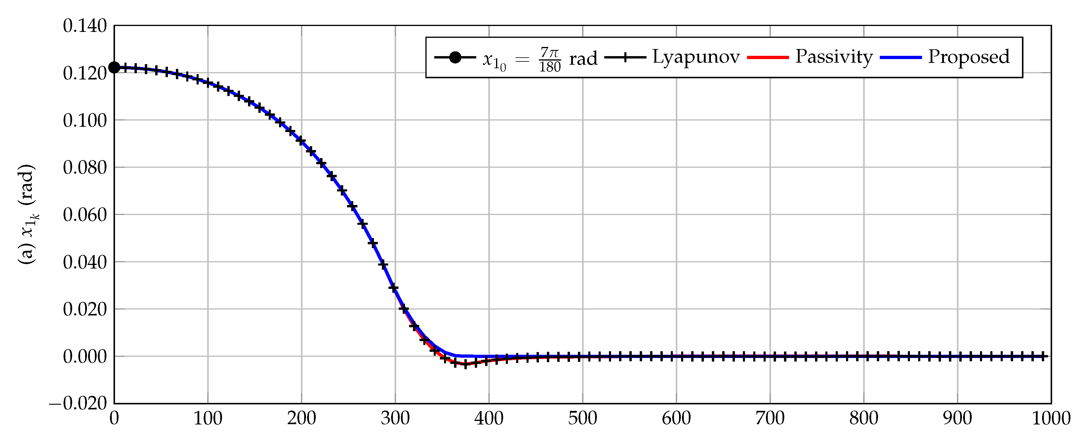
In Figure 5 is presented the comparison between the proposed inverse optimal controller and the Lyapunov-based design and the passivity-based approach reported in [4,5], respectively.

From Figure 5, we can state that the Lyapunov-based and the passivity-based approaches have the same numerical performances since the angular position are overlapped for both controllers. Furthermore, these controllers take about 470 ms to establish around the reference. In comparison, the proposed inverse optimal control approach outperforms all its counterparts reaching the reference signal in about 370 ms. It is worthy to mention that the comparative approaches present an overpass to the reference signal. This implies that some oscillations in the vertical position are experienced. Simultaneously, the proposed method does not present this behavior, which confirms its efficiency in contrast to powerful and well-known nonlinear approaches.

5. Conclusions and Future Works

This research addressed the global stabilization of a reaction wheel pendulum using the discrete-affine dynamical model with two state variables via control Lyapunov functions. The main advantages of the proposed control design are the following:

• The feedback control law $u_k^{\star }$ guarantees an exponential an asymptotically stable behavior with capabilities of working under parametric uncertainties without compromising the convergence to the equilibrium point in settling times lower than 700 ms.
• The control function is $u_k^{\star }$ is indeed an optimal signal since it minimizes the cost function and make it to reach the global optimum value of the cost functional at $V^{\star }\left(x_k\right)=\frac{1}{2}{x}_0^{T}P{x}_0$ with settling times between 370 ms and 700 ms.

Comparing the proposed controller with classical nonlinear controllers has demonstrated that the studied discrete inverse optimal controller via control Lyapunov functions can achieve global stabilization of the RWP system with exponential convergence. This is an advantage regarding classical passivity-based and Lyapunov-based depending on selecting the R gains and the values of the P matrix. Hence, it is possible to reach the equilibrium point with lower settling times.

As future works, the following developments could be considered: (i) to extend the formulation of the discrete-inverse optimal control via control Lyapunov functions to power electronic converters to integrate renewables and battery energy storage systems, and (ii) to apply the proposed controller to reduce frequency oscillations in power systems by improving controllers in synchronous machines.