Article

Nonstandard Finite Difference Schemes for the Study of the Dynamics of the Babesiosis Disease

1
Center for Informatics and Computing, Vietnam Academy of Science and Technology (VAST), 18 Hoang Quoc Viet, Cau Giay, Hanoi 100000, Vietnam
2
Institute of Information Technology, Vietnam Academy of Science and Technology (VAST), 18 Hoang Quoc Viet, Cau Giay, Hanoi 100000, Vietnam
3
Faculty of Science and Education, Universidad Distrital Francisco José de Caldas, Carrera 3 No. 26A - 40, Bogotá 11021-110231588, Colombia
4
Department of Mathematics, University of Castilla-La Mancha, Avda. de Espana, s/n, 02071 Albacete, Spain
*
Author to whom correspondence should be addressed.
Symmetry 2020, 12(9), 1447; https://doi.org/10.3390/sym12091447
Submission received: 16 July 2020 / Revised: 20 August 2020 / Accepted: 24 August 2020 / Published: 2 September 2020
(This article belongs to the Special Issue Advances in Nonlinear, Discrete, Continuous and Hamiltonian Systems)

Abstract

:
In this paper, a discrete-time model for Babesiosis disease, given by means of nonstandard finite difference (NSFD) schemes, is first provided and analyzed. Mathematical analyses show that the provided NSFD schemes preserve the essential (qualitative) dynamical properties of the continuous-time model, namely, positivity and boundedness of the solutions, equilibria, and their stability properties. In particular, the global stability of the disease free equilibrium point is proved by using an appropriate Lyapunov function. As a relevant consequence, we get the dynamic consistency of NSFD schemes in relation to the continuous-time model. Numerical simulations are presented to support the validity of the established theoretical results.

1. Introduction

The bovine babesiosis, caused by Babesia bovis and Babesia bigemina, is one of the most important vector-transmitted diseases. It is transmitted by the sting of ticks as the principal vector [1,2]. Babesiosis has an important economic impact in the livestock sector of tropical regions. Mathematical models for Babesiosis disease play an important role in both theory and practice. Therefore, these models have attracted the attention of many mathematicians, biologists, ecologists, and epidemiologists on several aspects, including the qualitative study (see in [3,4,5,6,7,8,9] and references therein) and the construction of adequate discretizations [10].
In this paper, we consider the well-known continuous-time mathematical model for Babesiosis disease proposed in [3], in order to construct nonstandard finite difference (NSFD) schemes, preserving the essential properties (i.e., positivity, boundedness, and stability) of the continuous-time model. It should be emphasized that the transformation of continuous models into discrete ones with the preservation of the essential properties is very important but not simple work. The most successful approach to the problem is the use of NSFD schemes. So far, NSFD schemes have been one of the most effective tools for this problem, as the majority of standard finite difference schemes can change and not preserve the properties of the continuous model [11] for any grid size. Notable results on NSFD for systems of ODEs can be found in [11,12,13,14,15,16,17,18,19,20]. There, the considered systems are the models of essential phenomena and processes arising in applied fields. Recently, some results on NSFD schemes for some ordinary and fractional differential equations have been obtained [21,22,23,24,25,26,27].
Returning to the work [3], notice that some stability properties of the model were established either theoretically or numerically. In [10], a discrete-time model for Babesiosis, which is in essence the Euler scheme with the unit step size, was studied and similar results of stability as in the continuous-time model were obtained either by rigorous proof or numerical simulations. Nevertheless, in the discrete case, the additional assumption of some parametric constrains was needed. Motivated by this work, in this paper, we construct discrete models for system (2) with all the stability properties established theoretically and illustrated by numerical examples. The numerical simulations also confirm the advantages of NSFD schemes over standard finite difference (SFD) schemes for large grid sizes.
By this occasion, we remark that a big challenge in the construction of NSFD schemes for continuous-time epidemic models is that the disease-free equilibrium point of the models is not only locally stable but also globally stable. Furthermore, when the reproduction number R 0 = 1 , it becomes a non-hyperbolic equilibrium point. Many continuous-time models considered before (see, e.g., in [11,13,14,15,16,20]) only deal with the local stability of hyperbolic equilibrium points. Here, by using an appropriate Lyapunov function, we prove that the disease-free equilibrium point is globally asymptotically stable if R 0 1 . As the main conclusion of this study, we get that NSFD schemes are dynamically consistent with the continuous model. On the other hand, our results in this paper constitute a generalization of those obtained in the recent work [10].
This paper is organized as follows. The mathematical model and its properties are recalled briefly in Section 2. Section 3 is devoted to the construction of NSFD schemes. Section 4 discusses the numerical simulations. Finally, there are some conclusions and discussions.

2. Mathematical Model

First, we consider the mathematical model for Babesiosis disease constructed in [3]. The dynamic transmission of Babesiosis disease for bovine and tick populations can be modeled by the following system of nonlinear first order differential equations,
S ¯ B ( t ) = μ B + α B C ¯ B ( t ) β B S ¯ B ( t ) I ¯ T ( t ) N T ( t ) , I ¯ B ( t ) = β B S ¯ B ( t ) I ¯ T ( t ) N T ( t ) λ B I ¯ B ( t ) , C ¯ B ( t ) = λ B I ¯ B ( t ) μ B + α B C ¯ B ( t ) , S ¯ T ( t ) = μ T p I ¯ T S ¯ T ( t ) I ¯ B ( t ) N B ( t ) , I ¯ T ( t ) = S ¯ T ( t ) I ¯ B ( t ) N B ( t ) μ T p I ¯ T ,
where the total population of bovine N B ( t ) is divided into three subpopulations: bovines which may become infected (Susceptible S ¯ B ( t ) ), bovines infected by the Babesia parasite (Infected I ¯ B ( t ) ), and bovines which have been treated for the Babesiosis (Controlled C ¯ B ( t ) ). That is, as in [3], N B = S B ¯ + I B ¯ + C B ¯ . The total population of ticks N T ( t ) is divided into two subpopulations: ticks which may become infected S ¯ T ( t ) and ticks infected by the Babesia parasite I ¯ T ( t ) . As in [3], the parameter μ B represents the birth rate of the bovines and it is assumed equal to their natural death; μ T is the birth rate of the ticks and it is also assumed equal to their death rate; any susceptible bovine can become infected due to a sting of an infected tick at a rate β B ; any susceptible tick can become infected when it stings an infected bovine, at a rate β T ; p is the probability for a susceptible tick to be born from an infected one; λ B represents the fraction of the infected bovines which are controlled, that is, treated against Babesia, while α B represents the fraction of the controlled bovines which may return to susceptible state. All these parameters in the model are positive and not exceeding 1, as this is biologically logical. More details on this model can be found in [3].
Below, we recall the main results of that work. In particular, after normalization of the variables, it was shown that system (1) is equivalent to subsystem
S B ( t ) = μ B + α B 1 S B ( t ) I B ( t ) β B S B ( t ) I T ( t ) , I B ( t ) = β B S B ( t ) I T ( t ) λ B I B ( t ) , I T ( t ) = β T 1 I T ( t ) I B ( t ) μ T p I T ( t )
and the region
Ω = S B , I B , I T R + 3 | 0 S B + I B 1 , 0 I T 1 ,
is a positive invariant set for the system (2). For this system, the threshold parameter is given by
R 0 = β B β T λ B μ T p .
Concerning system (2), the following results are obtained.
(i)
System (2) has the disease-free equilibrium point F 1 * = ( S B 1 * , I B 1 * , I T 1 * ) = ( 1 , 0 , 0 ) for all values of the parameters in this system, whereas, only if R 0 > 1 , there is a (unique) endemic equilibrium point F 2 * = ( S B 2 * , I B 2 * , I T 2 * ) in the interior of Ω given by
S B 2 * = β T λ B ( α B + μ B ) + p λ B ( α B + λ B + μ B ) μ T β T α B ( β B + λ B ) + λ B + μ B + β B ( λ B + μ B ) , I B 2 * = ( α B + μ B ) ( β B β T p λ B μ T ) β T α B ( β B + λ B ) + λ B + μ B + β B ( λ B + μ B ) , I T 2 * = ( α B + μ B ) ( β B β T p λ B μ T ) β T β B ( α B + μ B ) + p β B ( α B + λ B + μ B ) μ T .
(ii)
If R 0 1 , then the disease-free point F 1 * is globally asymptotically stable; otherwise, the disease-free point F 1 * is unstable.
(iii)
If R 0 > 1 , then the endemic point F 2 * is shown to be locally asymptotically stable by numerical simulations.
In [10], the authors proposed a discrete-time version of the continuous model (2) and obtained similar results of stability as for the continuous case. However, the additional assumption of some parametric constraints was required.

3. Nonstandard Finite Difference Schemes for System (2)

Our main goal is to construct NSFD schemes preserving the essential properties of the model (2). Let N be a positive integer and [ 0 , T ] be a finite interval. Let us denote by h = Δ t = T / N the time step size of the discretization:
0 = t 0 < t 1 < < t N = T = N h ,
and let t k = k h for k = 0 , 1 , , N . We now denote by S B k , I B k and I T k the approximated values of S B ( t k ) , I B ( t k ) and I T ( t k ) , respectively. Following the Mickens’ methodology, we propose NSFD schemes of the form
S B k + 1 S B k φ ( h ) = μ B + α B 1 S B k I B k β B S B k I T k , I B k + 1 I B k φ ( h ) = β B S B k I T k λ B I B k , I T k + 1 I T k φ ( h ) = β T 1 I T k I B k μ T p I T k ,
where φ ( h ) = h + O ( h 2 ) as h 0 . The conditions on φ ( h ) will be determined so that the properties of system (2) are preserved. For convenience, h is omitted in some presentations.
Theorem 1.
The set Ω defined by (3) is a positive invariant set of discrete model (6) if
φ ( h ) < min 1 β B , 1 λ B , 1 μ T p , 1 β T , 1 μ B + α B , h > 0 .
Proof. 
The theorem is proved by induction. First, rewrite system (6) in the form
S B k + 1 = S B k + φ μ B + α B 1 S B k I B k φ β B I T k S B k , I B k + 1 = I B k + φ β B S B k I T k φ λ B I B k , I T k + 1 = I T k + φ β T 1 I T k I B k φ μ T p I T k .
Clearly, if ( S B k , I B k , I T k ) Ω and condition (7) holds, then S B k + 1 0 , I B k + 1 0 and I T k + 1 0 . On the other hand, given ( S B k , I B k , I T k ) Ω , from the third equation of (8), we have
I T k + 1 I T k + φ β T 1 I T k = ( 1 φ β T ) I T k + φ β T 1 φ β T + φ β T = 1 .
Adding the first and second equations of (8), we obtain
S B k + 1 + I B k + 1 = S B k + I B k + φ μ B + α B 1 S B k I B k φ λ B I B k S B k + I B k + φ μ B + α B 1 S B k I B k = 1 φ ( μ B + α B ) ( S B k + I B k ) + φ ( μ B + α B ) 1 φ ( μ B + α B ) + φ ( μ B + α B ) = 1 .
Thus, the proof is complete. □
Similar to Proposition 1 in [3], we obtain the following result.
Corollary 1.
Model (6) has the disease-free equilibrium point F 1 * = ( S B * , I B * , I T * ) = ( 1 , 0 , 0 ) for all the values of the parameters in this model, whereas, only if R 0 > 1 , there is a (unique) endemic equilibrium point F 2 * = ( S B * , I B * , I T * ) in the interior of Ω, where the endemic point is given by (5).
Theorem 2.
Consider the model (6) under the assumption of Theorem 1.
(i) 
If R 0 1 , then the disease-free equilibrium point F 1 * is globally asymptotically stable.
(ii) 
If R 0 > 1 , then the disease-free equilibrium point F 1 * is unstable.
Proof. 
We shall distinguish two parts as in the statement of the theorems.
(i) 
We will use an extension for the discrete case (see in [28], Theorem 3.3) of the Lyapunov stability theorem [29] to prove this part. For this purpose, consider a function V : Ω R + defined by
V ( S B k , I B k , I T k ) : = β T I B k + λ B I T k .
Clearly, V is continuous, V S B k , I B k , I T k 0 for all S B k , I B k , I T k Ω , and V ( F 1 * ) = 0 .
From (6), we have
Δ V ( S B k , I B k , I T k ) : = V ( S B k + 1 , I B k + 1 , I T k + 1 ) V ( S B k , I B k , I T k ) = β T ( I B k + 1 I B k ) + λ B ( I T k + 1 I T k ) , = φ β T β B S B k I T k λ B I B k + φ λ B β T 1 I T k I B k μ T p I T k φ β T β B I T k λ B I B k + φ λ B β T 1 I T k I B k μ T p I T k = φ ( β T β B λ B μ T p ) I T k λ B β T I B k I T k φ ( β T β B λ B μ T p ) I T k = φ λ B μ T p ( R 0 1 ) I T k ,
which implies that Δ V 0 for all S B k , I B k , I T k Ω .
Let G * be the largest positively invariant set contained in
G : = S B k , I B k , I T k Ω | Δ V = 0 .
Then, by using (9) we have that
G * = F 1 * if R 0 < 1 , ( 0 , 0 , I T k ) | I T k 0 if R 0 = 1 .
Consequently, it is easy to verify that F 1 * is G * -globally asymptotically stable if R 0 1 .
As all solutions of (6) are bounded, by (see in [28], Theorem 3.3) we deduce that F 1 * is globally asymptotically stable if R 0 1 .
(ii) 
Computing the Jacobian matrix of system (6) evaluated at the disease free point, one obtains
J ( 1 , 0 , 0 ) = 1 φ ( α B + μ B ) φ ( α B + μ B ) φ β B , 0 1 φ λ B φ β B 0 φ β T 1 φ μ T p .
Consequently, the eigenvalues of J ( F 1 * ) are Λ 1 = 1 φ ( α B + μ B ) and Λ 2 , Λ 3 , where Λ 2 , Λ 3 are the eigenvalues of
J 1 = 1 φ λ B φ β B φ β T 1 φ μ T p .
We have
det ( J 1 ) = 1 φ ( λ B + μ T p ) φ 2 λ B μ T p ( R 0 1 ) , T r ( J 1 ) = 2 φ ( λ B + μ T p ) .
Thus, if R 0 > 1 , then 1 T r ( J 1 ) + det ( J 1 ) = φ 2 λ B μ T p ( R 0 1 ) < 0 . By Theorem 1.3.7 in [30] and Theorem 2.10 in [31], we can conclude that if R 0 > 1 then the disease-free equilibrium point F 1 * is unstable.
Thus, the theorem is proved. □
Next, we shall investigate the local stability of system (6) in the case R 0 > 1 . Denote by σ ( J ) the set of eigenvalues of the Jacobian matrix J of system (2) at F 2 * . Based on mathematical analyses in [3], we have if R 0 > 1 then F 2 * is locally asymptotically stable and the eigenvalues of J lie within the left half of the complex plane, i.e.,
R e ( Λ i ) < 0 , Λ i σ ( J ) , i = 1 , 2 , 3 .
Now we denote by K the Jacobian matrix of system (6) at F 2 * . Then K = I + φ J (see [13,14]), where I is 3 × 3 unit matrix. Therefore, the eigenvalues Λ i of J correspond to the eigenvalues Ψ i of K determined by
Ψ i = 1 + φ Λ i , i = 1 , 2 , 3 .
By Lyapunov indirect method for discrete dynamical systems (see ([30], Theorem 1.3.7) and [31]), F 2 * is locally asymptotically stable of system (6) if and only if
| Ψ i | < 1 , i = 1 , 2 , 3 .
This is equivalent to
| Ψ i | 2 = | 1 + φ Λ i | 2 = φ 2 I m 2 ( Λ i ) + 1 + 2 φ R e ( Λ i ) + φ 2 R e 2 ( Λ i ) < 1 , i = 1 , 2 , 3 .
The above inequality is satisfied if
φ < 2 R e ( Λ i ) | Λ i | 2 , i = 1 , 2 , 3 .
Conversely, if R 0 1 , then F 2 * has no biological sense. Thus, it has no biological sense to study its stability.
From the above results, we have the following theorem.
Theorem 3.
Consider system (6) when R 0 > 1 . Suppose Λ 1 , Λ 2 , Λ 3 are the eigenvalues of the Jacobian matrix of system (2) at F 2 * . Set
τ * : = min i = 1 , 2 , 3 2 R e ( Λ i ) | Λ i | 2 .
Then, F 2 * is locally asymptotically stable if
0 < φ ( h ) < τ * , h > 0 .
Summing up the results of this section, we obtain the following theorem.
Theorem 4 (Dynamically consistent discrete models).
Consider NSFD scheme (6).
(i) 
In the case R 0 1 , scheme (6) preserves positivity, boundedness, and global stability of F 1 * of system (2) if
0 < φ ( h ) < φ * : = min 1 β B , 1 λ B , 1 μ T p , 1 β T , 1 μ B + α B , h > 0 .
(ii) 
In the case R 0 > 1 , scheme (6) preserves positivity, boundedness and local stability of F 2 * and unstability of F 1 * if
0 < φ ( h ) < φ * : = min 1 β B , 1 λ B , 1 μ T p , 1 β T , 1 μ B + α B , τ * , h > 0 ,
where τ * is given by (10).
Remark 1.
Concerning Theorem 2, we have to underline three important observations:
  • Part (i) of Theorem 2 is only appropriate when Ω is a positively invariant set of (6).
  • There are many ways for selecting the function φ ( h ) satisfying the conditions of Theorem 4, for example (see in [11,13,14,15,16]),
    φ ( h ) = 1 e T * h T * , T * > 1 φ * .
  • In the case of φ ( h ) = 1 , then scheme (6) becomes the discrete model which was proposed and studied in [10]. This proves that NSFD schemes (6) constitute a generalization of the discrete-time model in [10].

4. Numerical Simulations

We present some numerical simulations to illustrate the obtained theoretical results. From the numerical simulations, it will be shown that standard finite difference schemes (SFDS) may not preserve essential properties of the continuous-time model for any finite step size. Meanwhile, NSFD schemes preserve essential properties of continuous model for any finite step size.
Example 1 (Dynamics of standard finite difference schemes).
Consider system (2) with the parameters
μ B = 0.2999 , μ T = 0.8 , λ B = 0.265 , α B = 0.1 , p = 0.8 , β B = 0.1 , β T = 0.48 ,
subject to the initial value
S B ( 0 ) = 0.1 , I B ( 0 ) = 0.2 , I T ( 0 ) = 0.1 ,
and t [ 0 , 10 5 ] .
In this case, R 0 = 0.2830 < 1 and F 1 * = ( 1 , 0 , 0 ) is globally asymptotically stable. We use the Euler scheme, the classical fourth-stages Runge–Kutta (RK4) scheme and NSFD schemes (6) to numerically solve system (2). The numerical solutions obtained by these schemes are presented in Figure 1. From this figure, we see that the numerical solutions obtained by the Euler scheme and the RK4 schemes are not positive, their boundedness is destroyed. The Euler scheme gives the numerical solutions oscillating near the equilibrium points. Meanwhile, the numerical solution obtained by NSFD schemes preserve the essential properties of the model (2). Besides, the NSFD schemes is easily realized. It is the advantages of the NSFD schemes compared with standard difference schemes. Other examples give the same results. This fact completely agrees with several results in the previous works [11,13,14,15,20,21,22,23].
Example 2 (Dynamics of NSFD schemes in the case R 0 1 ).
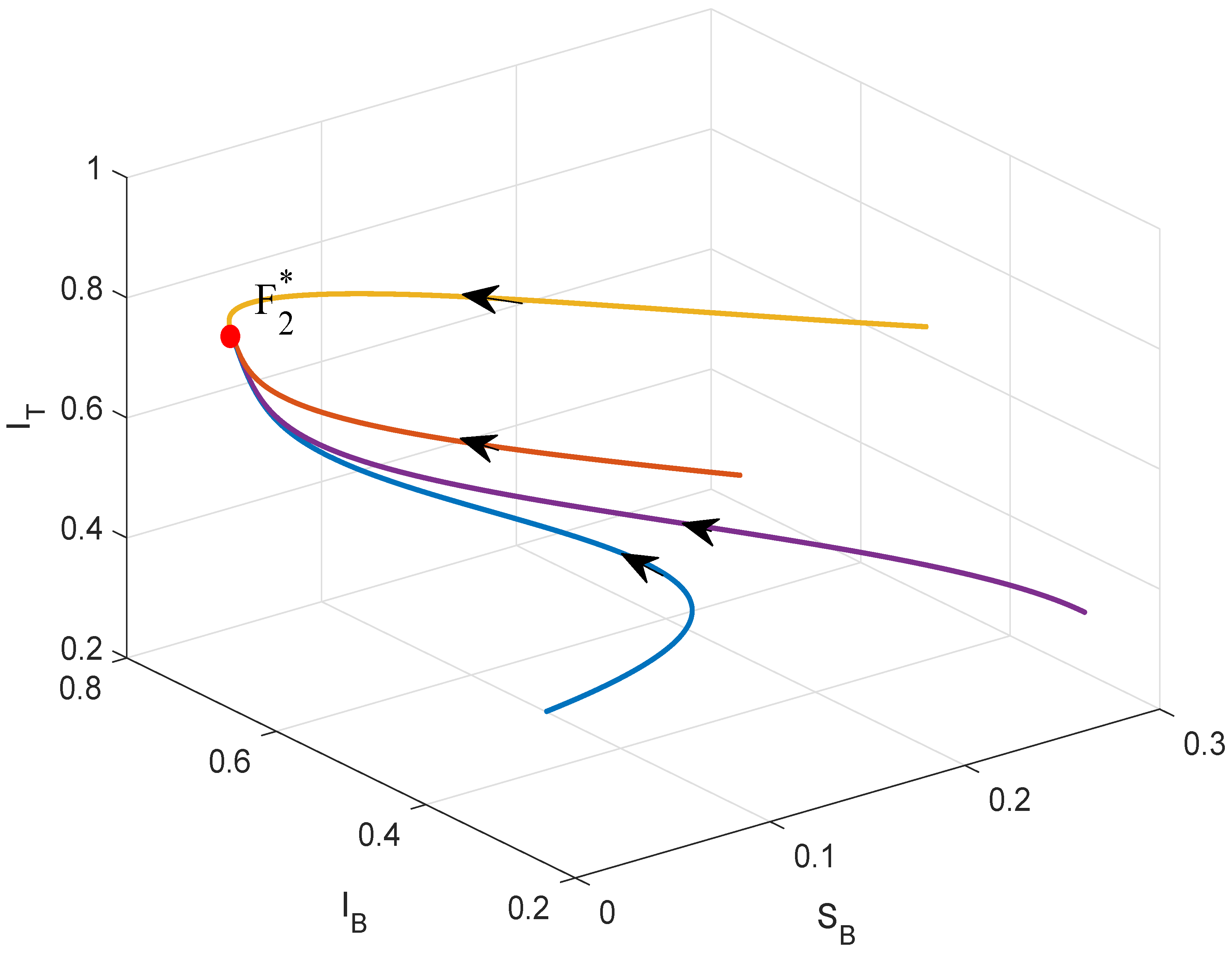
Consider system (2) with the parameters (see in [3])
μ B = 0.0002999 , μ T = 0.001609 , λ B = 0.0265 , α B = 0.001 , p = 0.1 , β B = 0.003 , β T = 0.00048 .
In this case, R 0 = 0.33 and the number φ * in Theorem 4 is φ * = 37.7358 . Therefore, we take
φ ( h ) = 1 e 0.03 h 0.03 .
Numerical solutions obtained from this NSFD scheme (6) is depicted in Figure 2. Clearly, the properties of the continuous-time model are preserved.
Example 3 (Dynamics of NSFD schemes in the case R 0 > 1 ).
Consider system (2) with the parameters (see in [3])
μ B = 0.0002999 , μ T = 0.001609 , λ B = 0.000265 , α B = 0.001 , p = 0.1 , β B = 0.006 , β T = 0.00048 .
In this case, R 0 = 67.54 and the number φ * in Theorem 4 is φ * = 166.67 . Therefore, we take
φ ( h ) = 1 e 0.005 h 0.005 .
Numerical solutions obtained from this NSFD scheme (6) is depicted in Figure 3. Similar to Example 2, the properties of the continuous-time model are preserved.

5. Conclusions

As the main conclusion of this study, we obtain the dynamic consistency of NSFD schemes in relation to the continuous-time model. That is, NSFD schemes preserve essential properties of the continuous-time model, while standard finite difference schemes (SFDS) cannot preserve these properties.
On the other hand, it is worth to note that our results constitute a generalization of those in [10].
In future works, the results in this paper will be useful in order to develop other essential applied models, specially those models possessing non-hyperbolic equilibrium points with global stability property.

Supplementary materials

Supplementary File 1

Author Contributions

Conceptualization, Q.A.D., M.T.H., D.Y.T. and J.C.V.; Methodology, Q.A.D., M.T.H., D.Y.T. and J.C.V.; Software, Q.A.D., M.T.H., D.Y.T. and J.C.V.; Validation, Q.A.D., M.T.H., D.Y.T. and J.C.V.; Formal Analysis, Q.A.D., M.T.H., D.Y.T. and J.C.V.; Investigation, Q.A.D., M.T.H., D.Y.T. and J.C.V.; Resources, Q.A.D., M.T.H., D.Y.T. and J.C.V.; Data Curation, Q.A.D., M.T.H., D.Y.T. and J.C.V.; Writing—Original Draft Preparation, Q.A.D., M.T.H., D.Y.T. and J.C.V.; Writing—Review and Editing, Q.A.D., M.T.H., D.Y.T. and J.C.V. All authors contributed equally to the paper. All authors have read and agreed to the published version of the manuscript.

Funding

D.Y.T. has performed this work within the specific educational cooperation agreement for fellowships in doctoral programs and short research stays for professors with doctorates between the Fundación Carolina, Spain and the University Francisco José de Caldas, Colombia. She has also been supported by the Doctoral Study Commission Grant from the University Francisco José de Caldas, by Superior [Resolution 038 of 2016]. J.C.V. was funded by FEDER OP2014-2020 of Castilla-La Mancha (Spain) [grant number 2020-GRIN-29225] and by the Ministry of Science, Innovation and Universities of Spain [grant number PGC2018-097198-B-I00].

Conflicts of Interest

The authors declare no conflict of interest.

Data Availability

The data used to support the findings of this study are included within the article.

References

  1. Solorio-Rivera, J.L.; Rodriguez-Vivas, R.I. Epidemiology of bovine babesiosis. I. Epidemiological Components. Rev. Biomed. 1997, 8, 37–47. [Google Scholar]
  2. Solorio-Rivera, J.L.; Rodriguez-Vivas, R.I. Epidemiology of the babesiosis bovis. II. Epidemiologic indicators and elements for the design of strategies of control. Rev. Biomed. 1997, 8, 95–105. [Google Scholar]
  3. Aranda, D.F.; Trejos, D.Y.; Valverde, J.C.; Villanueva, R.-J. A mathematical model for Babesiosis disease in bovine and tick populations. Math. Methods Appl. Sci. 2011, 35, 249–256. [Google Scholar] [CrossRef]
  4. Bouzid, L.; Belhamiti, O. Effect of seasonal changes on predictive model of bovine babesiosis transmission. Int. J. Model. Simul. Sci. Comput. 2017, 8, 1750030. [Google Scholar] [CrossRef]
  5. Carvalho dos Santos, J.P.; Cardoso, L.C.; Monteiro, E.; Lemes, N.H.T. A Fractional-Order Epidemic Model for Bovine Babesiosis Disease and Tick Populations. Abstr. Appl. Anal. 2015, 2015, 729894. [Google Scholar] [CrossRef]
  6. Friedman, A.; Yakubu, A.-A. A Bovine Babesiosis Model with Dispersion. Bull. Math. Boil. 2013, 76, 98–135. [Google Scholar] [CrossRef]
  7. Pourbashash, H. Global Analysis of the Babesiosis Disease in Bovine and Tick Populations Model and Numerical Simulation with Multistage Modified Sinc Method. Iran. J. Sci. Technol. Trans. A Sci. 2018, 42, 39–46. [Google Scholar] [CrossRef]
  8. Saad-Roy, M.C.; Shuai, Z.; Van den Driessche, P. Driessche, Models of bovine Babesiosis including juvenile cattle. Bull. Math. Biol. 2015, 77, 514–547. [Google Scholar] [CrossRef]
  9. Zafar, Z.U.A.; Rehan, K.; Mushtaq, M. Fractional-order scheme for bovine babesiosis disease and tick populations. Adv. Differ. Equ. 2017, 2017, 4. [Google Scholar] [CrossRef] [Green Version]
  10. Aranda, D.F.; Trejos-Angel, D.Y.; Valverde, J.C. A discrete epidemic model for bovine Babesiosis disease and tick populations. Open Phys. 2017, 15, 360–369. [Google Scholar] [CrossRef]
  11. Mickens, R.E. Applications of Nonstandard Finite Difference Schemes; World Scientific: Singapore, 2000. [Google Scholar]
  12. Adekanye, O.; Washington, T. Nonstandard finite difference scheme for a Tacoma Narrows Bridge model. Appl. Math. Model. 2018, 62, 223–236. [Google Scholar] [CrossRef]
  13. Dimitrov, D.T.; Kojouharov, H.V. Stability-Preserving Finite-Difference Methods For General Multi-Dimensional Autonomous Dynamical Systems. Int. J. Numer. Anal. Model 2007, 4, 280–290. [Google Scholar]
  14. Dimitrov, D.T.; Kojouharov, H.V. Nonstandard finite-difference schemes for general two-dimensional autonomous dynamical systems. Appl. Math. Lett. 2005, 18, 769–774. [Google Scholar] [CrossRef] [Green Version]
  15. Dimitrov, D.T.; Kojouharov, H.V. Positive and elementary stable nonstandard numerical methods with applications to predator–prey models. J. Comput. Appl. Math. 2006, 189, 98–108. [Google Scholar] [CrossRef] [Green Version]
  16. Dimitrov, D.T.; Kojouharov, H.V. Nonstandard finite-difference methods for predator–prey models with general functional response. Math. Comput. Simul. 2008, 78, 1–11. [Google Scholar] [CrossRef]
  17. Gurski, K.F. A simple construction of nonstandard finite-difference schemes for small nonlinear systems applied to SIR models. Comput. Math. Appl. 2013, 66, 2165–2177. [Google Scholar] [CrossRef]
  18. Korpusik, A. A nonstandard finite difference scheme for a basic model of cellular immune response to viral infection. Commun. Nonlinear Sci. Numer. Simul. 2017, 43, 369–384. [Google Scholar] [CrossRef]
  19. Roeger, L.-I.W.; Gelca, R. Dynamically Consistent Discrete-Time Lotka-Volterra Competition Models. In Proceedings of the 7th AIMS International Conference, Arlington, TX, USA, 18–21 May 2009; pp. 650–658. [Google Scholar]
  20. Wood, D.; Kojouharov, H.V. A class of nonstandard numerical methods for autonomous dynamical systems. Appl. Math. Lett. 2015, 50, 78–82. [Google Scholar] [CrossRef]
  21. Dang, Q.A.; Hoang, M.T. Dynamically consistent discrete metapopulation model. J. Differ. Equ. Appl. 2016, 22, 1325–1349. [Google Scholar] [CrossRef]
  22. Dang, Q.A.; Hoang, M.T. Lyapunov direct method for investigating stability of nonstandard finite difference schemes for metapopulation models. J. Differ. Equ. Appl. 2017, 24, 32–47. [Google Scholar] [CrossRef] [Green Version]
  23. Dang, Q.A.; Hoang, M.T. Complete Global Stability of a Metapopulation Model and Its Dynamically Consistent Discrete Models. Qual. Theory Dyn. Syst. 2018, 18, 461–475. [Google Scholar] [CrossRef]
  24. Dang, Q.A.; Hoang, M.T. Nonstandard finite difference schemes for a general predator–prey system. J. Comput. Sci. 2019, 36, 101015. [Google Scholar] [CrossRef] [Green Version]
  25. Dang, Q.A.; Hoang, M.T. Positivity and global stability preserving NSFD schemes for a mixing propagation model of computer viruses. J. Comput. Appl. Math. 2020, 374, 112753. [Google Scholar] [CrossRef]
  26. Dang, Q.A.; Hoang, M.T. Positive and elementary stable explicit nonstandard Runge-Kutta methods for a class of autonomous dynamical systems. Int. J. Comput. Math. 2019. [Google Scholar] [CrossRef] [Green Version]
  27. Hoang, M.T.; Nagy, A.M. Uniform asymptotic stability of a Logistic model with feedback control of fractional order and nonstandard finite difference schemes. Chaos Solitons Fractals 2019, 123, 24–34. [Google Scholar] [CrossRef]
  28. Iggidr, A.; Bensoubaya, M. New Results on the Stability of Discrete-Time Systems and Applications to Control Problems. J. Math. Anal. Appl. 1998, 219, 392–414. [Google Scholar] [CrossRef] [Green Version]
  29. LaSalle, J.P. The Stability of Dynamical Systems; SIAM: Philadelphia, PA, USA, 1976. [Google Scholar]
  30. Stuart, A.M.; Humphries, A.R. Dynamical Systems and Numerical Analysis, Cambridge Monographs on Applied and Computational Mathematics; Cambridge University Press: Cambridge, UK, 1996. [Google Scholar]
  31. Allen, L.J.S. An Introduction to Mathematical Biology; Prentice Hall: Upper Saddle River, NJ, USA, 2007. [Google Scholar]
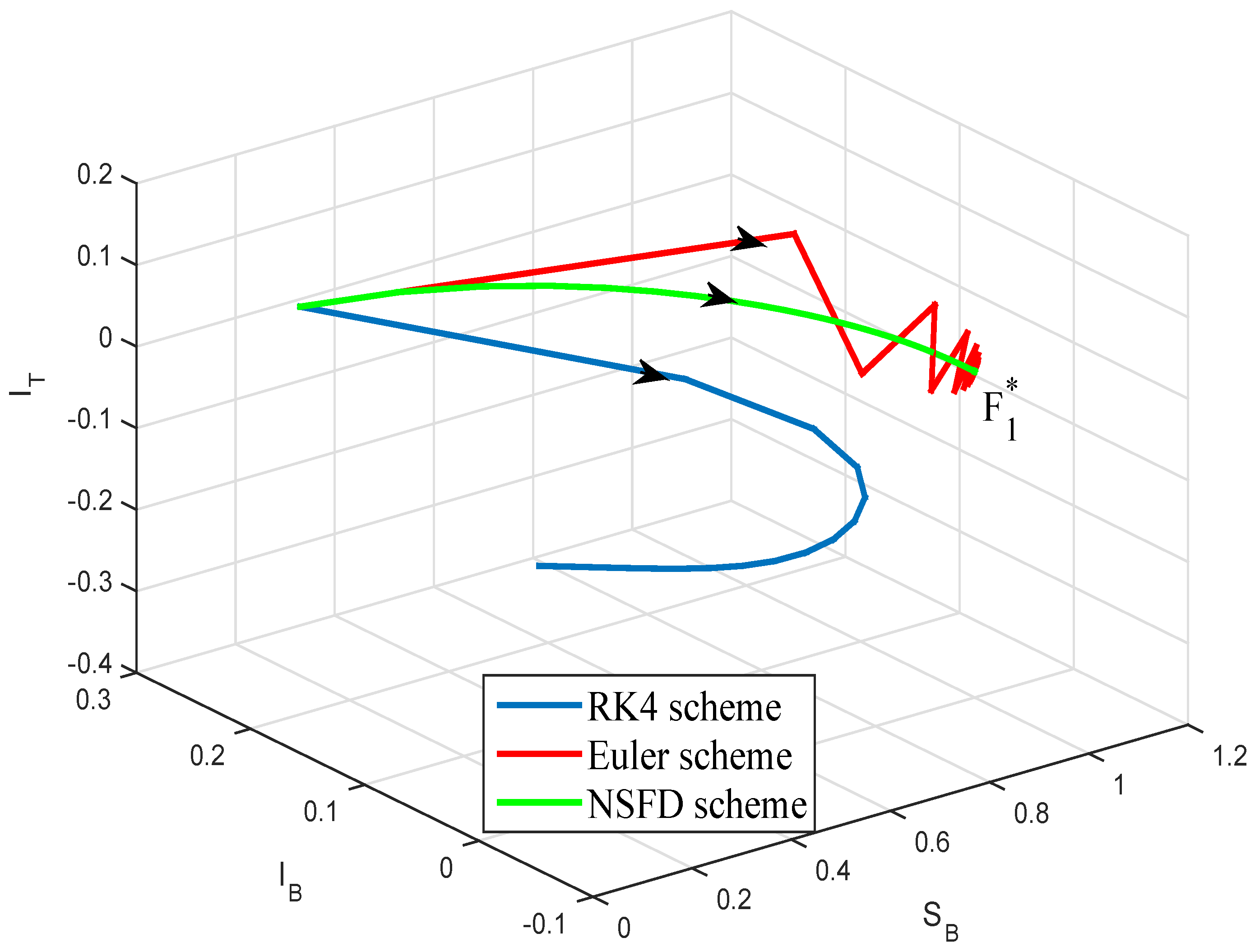
Figure 1. Numerical solutions obtained by the RK4 scheme (with h = 4 ), the Euler scheme (with h = 2.5 ) and NSFD scheme (with h = 5 and φ ( h ) = ( 1 e 2 h ) / 2 ) in Example 1.
Symmetry 12 01447 g001
Figure 2. Numerical solutions in Example 2 with h = 1 and t [ 0 , 5 × 10 5 ] .
Symmetry 12 01447 g002
Figure 3. Numerical solutions in Example 3 with h = 1 and t [ 0 , 10 3 ] .
Symmetry 12 01447 g003