Maritime Autonomous Surface Ship’s Path Approximation Using Bézier Curves


Abstract
1. Introduction
- –
- ship motion pattern based on the Latent Dirichlet Allocation model [8], which is based on trajectory datasets represented as limited series of motion words and needs big amount of data to give reliable model;
- –
- probabilistic model of the ship handling behavior patterns in the Automatic Identification System (AIS) data using the sub-trajectory clustering algorithm [9], where the AIS data is processed to get ship handling behavior basics;
- –
- spline model for trajectory estimation based on the AIS data [10], where AIS data needs to be filtered and then may be used to map ship’s maneuverability;
- –
- deterministic model based on the concept of a predefined trajectories database containing safe and optimal paths of a ship [11];
- –
- model determined by density-based spatial clustering of applications with the noise (DBSCAN) algorithm combined with the Artificial Neural Network learning relationship of turning regions and generating a feasible route based on massive AIS data [12],
- –
- using Bézier curves [13], which seems to be the least computationally complex and parameterizable.
2. Materials And Methods
2.1. Problem Statement
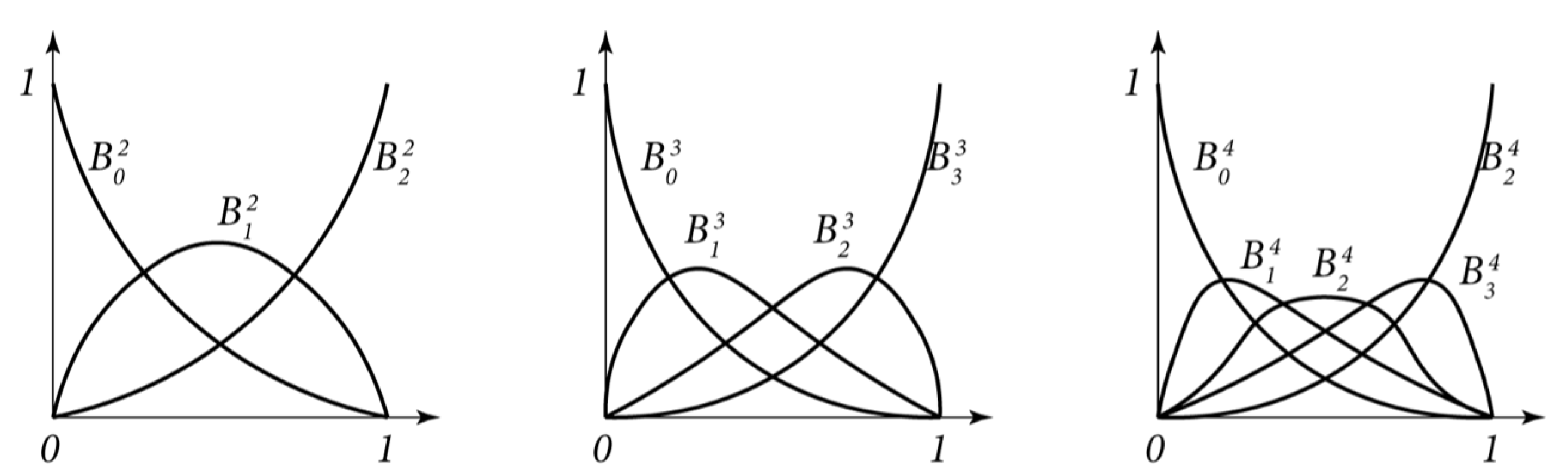
2.2. Bézier Curves
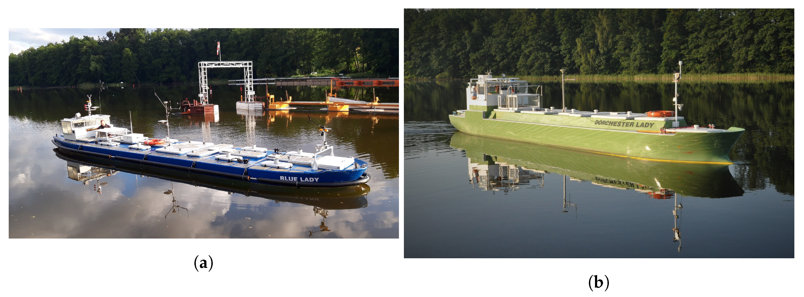
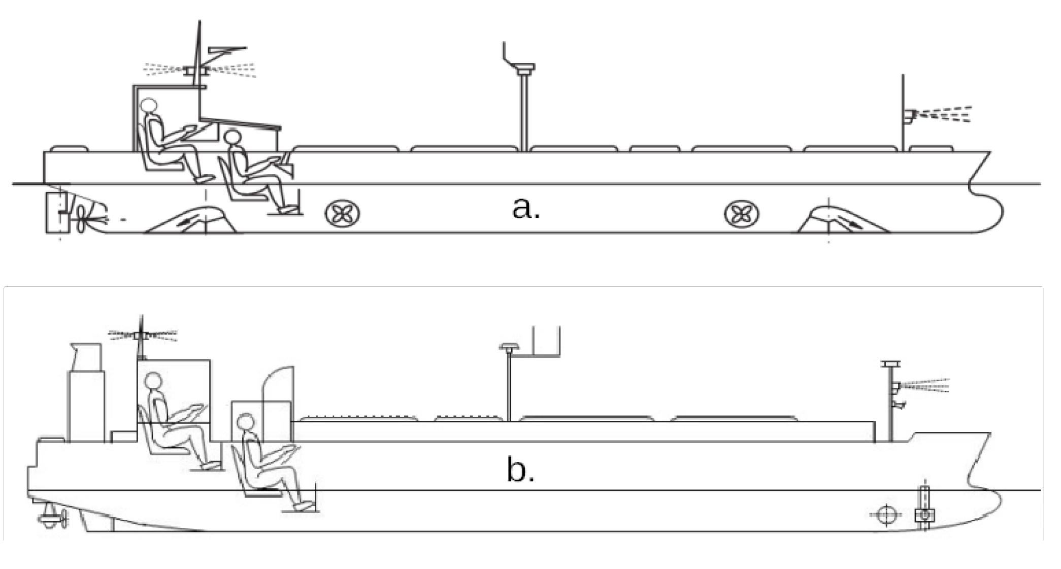
2.3. Test Bed—Training Ships
2.4. Method of Rational Bézier Curve Coefficient Determination
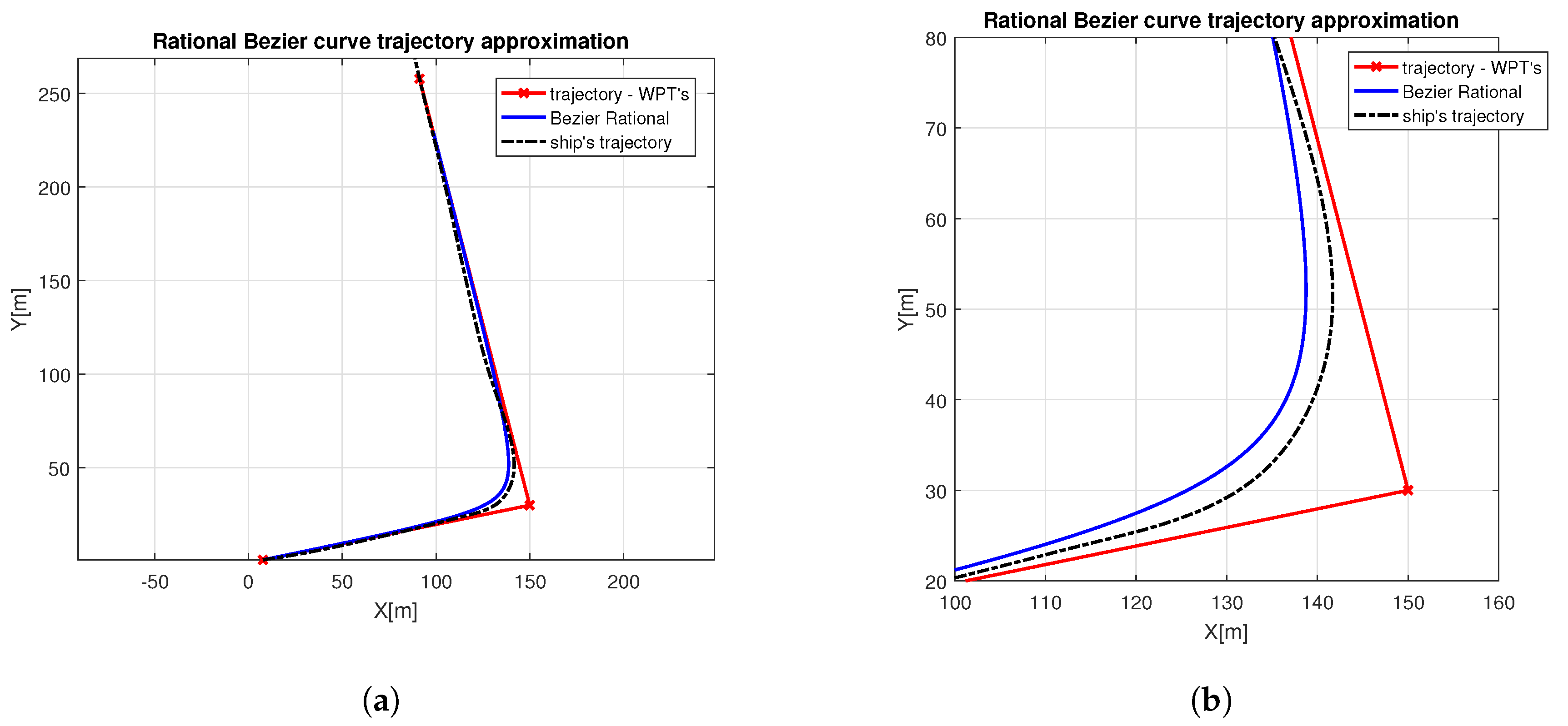
3. Results
4. Discussion
5. Conclusions
Author Contributions
Funding
Conflicts of Interest
References
- Plessen, M.M.G.; Bemporad, A. Reference trajectory planning under constraints and path tracking using linear time-varying model predictive control for agricultural machines. Biosyst. Eng. 2017, 153, 28–41. [Google Scholar] [CrossRef]
- Dixit, S.; Montanaro, U.; Fallah, S.; Dianati, M.; Oxtoby, D.; Mizutani, T.; Mouzakitis, A. Trajectory planning for autonomous high-speed overtaking using MPC with terminal set constraints. In Proceedings of the 2018 21st International Conference on Intelligent Transportation Systems (ITSC), Maui, HI, USA, 4–7 November 2018; pp. 1061–1068. [Google Scholar]
- Nolte, M.; Rose, M.; Stolte, T.; Maurer, M. Model predictive control based trajectory generation for autonomous vehicles—an architectural approach. In Proceedings of the 2017 IEEE Intelligent Vehicles Symposium (IV), Los Angeles, CA, USA, 11–14 June 2017; pp. 798–805. [Google Scholar]
- Xi, W.; Baras, J.S. MPC based motion control of car-like vehicle swarms. In Proceedings of the 2007 Mediterranean Conference on Control & Automation, Athens, Greece, 27–29 June 2007; pp. 1–6. [Google Scholar]
- Hu, Q.; Xie, J.; Wang, C. Dynamic path planning and trajectory tracking using MPC for satellite with collision avoidance. ISA Trans. 2019, 84, 128–141. [Google Scholar] [CrossRef] [PubMed]
- Shi, J.; Sun, D.; Qin, D.; Hu, M.; Kan, Y.; Ma, K.; Chen, R. Planning the trajectory of an autonomous wheel loader and tracking its trajectory via adaptive model predictive control. Robot. Auton. Syst. 2020, 131, 103570. [Google Scholar] [CrossRef]
- Cagienard, R.; Grieder, P.; Kerrigan, E.C.; Morari, M. Move blocking strategies in receding horizon control. J. Process Control 2007, 17, 563–570. [Google Scholar] [CrossRef]
- Huang, L.; Wen, Y.; Guo, W.; Zhu, X.; Zhou, C.; Zhang, F.; Zhu, M. Mobility pattern analysis of ship trajectories based on semantic transformation and topic model. Ocean Eng. 2020, 201, 107092. [Google Scholar] [CrossRef]
- Gao, M.; Shi, G.Y. Ship-handling behavior pattern recognition using AIS sub-trajectory clustering analysis based on the T-SNE and spectral clustering algorithms. Ocean Eng. 2020, 205, 106919. [Google Scholar] [CrossRef]
- Zhang, L.; Meng, Q.; Xiao, Z.; Fu, X. A novel ship trajectory reconstruction approach using AIS data. Ocean Eng. 2018, 159, 165–174. [Google Scholar] [CrossRef]
- Lazarowska, A. A new deterministic approach in a decision support system for ship’s trajectory planning. Expert Syst. Appl. 2017, 71, 469–478. [Google Scholar] [CrossRef]
- Wen, Y.; Sui, Z.; Zhou, C.; Xiao, C.; Chen, Q.; Han, D.; Zhang, Y. Automatic ship route design between two ports: A data-driven method. Appl. Ocean Res. 2020, 96, 102049. [Google Scholar] [CrossRef]
- Hassani, V.; Lande, S.V. Path planning for marine vehicles using Bezier curves. IFAC Pap. 2018, 51, 305–310. [Google Scholar] [CrossRef]
- Yang, G.J.; Choi, B.W. Smooth trajectory planning along Bezier curve for mobile robots with velocity constraints. Int. J. Control Autom. 2013, 6, 225–234. [Google Scholar]
- Choi, J.W.; Curry, R.; Elkaim, G. Path planning based on bézier curve for autonomous ground vehicles. In Proceedings of the Advances in Electrical and Electronics Engineering-IAENG Special Edition of the World Congress on Engineering and Computer Science 2008, San Francisco, CA, USA, 22–24 October 2008; pp. 158–166. [Google Scholar]
- Chen, L.; Wang, S.; Hu, H.; McDonald-Maier, K. Bézier curve based trajectory planning for an intelligent wheelchair to pass a doorway. In Proceedings of the 2012 UKACC International Conference on Control, Cardiff, UK, 3–5 September 2012; pp. 339–344. [Google Scholar]
- Yu, W.; Shuo, W.; Rui, W.; Min, T. Generation of temporal–spatial Bezier curve for simultaneous arrival of multiple unmanned vehicles. Inf. Sci. 2017, 418, 34–45. [Google Scholar] [CrossRef]
- Gierusz, W.; Miller, A. Ship Motion Control System for Replenishment Operation. In Applied Mechanics and Materials; Trans Tech Publ.: Zurich, Switzerland, 2016; pp. 214–222. [Google Scholar]
- Kiciak, P. Podstawy Modelowania Krzywych i Powierzchni: Zastosowania w Grafice Komputerowej; Wydawnictwa Naukowo-Techniczne/Wydawnictwo Naukowe PWN: Warszawa, Poland, 2019. [Google Scholar]
- Rybczak, M. Improvement of control precision for ship movement using a multidimensional controller. Automatika 2018, 59, 63–70. [Google Scholar] [CrossRef]
- Tomera, M. Hybrid real-time way-point controller for ships. In Proceedings of the 2016 21st International Conference on Methods and Models in Automation and Robotics (MMAR), Miedzyzdroje, Poland, 29 August–1 September 2016; pp. 630–635. [Google Scholar]
- Tomera, M. Sterowanie modelem fizycznym zbiornikowca wzdłuż zadanej trasy przejścia. Zeszyty Naukowe Wydziału Elektrotechniki i Automatyki Politechniki Gdańskiej 2016, 51, 201–208. [Google Scholar]


| VLCC | LNG Carrier | |
|---|---|---|
| “Blue Lady” | “Dorchester Lady” | |
| Length overall L [m] | 13.78 | 11.33 |
| Breadth B [m] | 2.38 | 1.80 |
| Draft T [m] | 0.86 | 0.50 |
| Displacement D [T] | 22.83 | 8.21 |
| Max. speed u [kn] | 3.10 | 3.20 |
| ex. | max. | c | angular | drift | ||
|---|---|---|---|---|---|---|
| error [m] | coef. [–] | path [m] | path [m] | coef. [–] | coef. [–] | |
| VLCC 1 | 3.1 | 0.65 | 116.46 | 27.99 | 3.65 | 0.52 |
| VLCC 2 | 4.0 | 0.46 | 73.96 | 15.03 | 2.76 | 0.60 |
| LNG 1 | 1.5 | 0.61 | 64.79 | 19.99 | 5.99 | 0.41 |
| LNG 2 | 1.3 | 0.57 | 103.17 | 31.41 | 5.41 | 0.43 |
| LNG 3 | 0.5 | 0.50 | 98.18 | 28.06 | 4.96 | 0.45 |
Publisher’s Note: MDPI stays neutral with regard to jurisdictional claims in published maps and institutional affiliations. |
© 2020 by the authors. Licensee MDPI, Basel, Switzerland. This article is an open access article distributed under the terms and conditions of the Creative Commons Attribution (CC BY) license (http://creativecommons.org/licenses/by/4.0/).
Share and Cite
Miller, A.; Walczak, S. Maritime Autonomous Surface Ship’s Path Approximation Using Bézier Curves. Symmetry 2020, 12, 1704. https://doi.org/10.3390/sym12101704
Miller A, Walczak S. Maritime Autonomous Surface Ship’s Path Approximation Using Bézier Curves. Symmetry. 2020; 12(10):1704. https://doi.org/10.3390/sym12101704
Chicago/Turabian StyleMiller, Anna, and Szymon Walczak. 2020. "Maritime Autonomous Surface Ship’s Path Approximation Using Bézier Curves" Symmetry 12, no. 10: 1704. https://doi.org/10.3390/sym12101704
APA StyleMiller, A., & Walczak, S. (2020). Maritime Autonomous Surface Ship’s Path Approximation Using Bézier Curves. Symmetry, 12(10), 1704. https://doi.org/10.3390/sym12101704