Abstract
Hepatitis B is a widespread epidemic in the world, but so far no single drug has been shown to kill or eliminate the Hepatitis B virus and heal people with chronic Hepatitis B virus infection. Based on comprehensive investigations to relevant characteristics of Hepatitis B, a diagnostic modelling and reasoning methodology using Dynamic Uncertain Causality Graph is proposed. The symptoms, physical signs, examinations results, medical histories, etiology, pathogenesis and other factors were included in the diagnosis model. In order to reduce the difficulty of building the model, a modular modeling scheme is proposed, which provides multi-perspectives and arbitrary granularity for the expression of disease causality. The chain reasoning algorithm and weighted logic operation mechanism are introduced to ensure the correctness and effectiveness of diagnostic reasoning under incomplete and uncertain information. In addition, the causal view of the potential interactions between diseases and symptoms visually shows the reasoning process in a graphical way. In the relevant model, the model of the diagnostic process and the model of the therapeutic process are symmetrical. The results show that, even with incomplete observations, the proposed methodology achieves encouraging diagnostic accuracy and effectiveness, providing a promising assistance tool for physicians in the diagnosis of Hepatitis B.
1. Introduction
Hepatitis B is a kind of infectious disease which spreads widely all over the world. As published by the World Gastroenterology Organization, more than 400 million people have been infected with hepatitis B, which is the third leading cause of cancer death in the world [1]. However, until now, there is no drug available for the hepatitis B virus elimination and to cure the chronic hepatitis B virus-infected patients. In response to this disease, researchers have made active efforts, aiming to improve the accuracy of diagnosis and provide more accurate treatment plans.
In recent years, with the development of computer science and artificial intelligence, it is possible to digitize medical diagnosis. Currently, the application of computer technology, in particular the artificial intelligence in medical diagnosis, has become one of the hot spots in the research society. Various decision making systems for medical diagnosis have been developed [2,3]. Moreover, computer-aided systems for clinical diagnoses have been involved in many major medical areas. These works promotes the development of medical science [4,5,6,7].
Rule reasoning method was first applied in clinical diagnosis, and has been widely used, such as MYCIN and INTERNIST-1 [8,9]. Various mixed reasoning method has also been adopted in clinical diagnosis and treatment decision making, such as method combining case-based and rule-based reasoning [10], method combining rule and neural network [11], method combining hybrid fuzzy logic and case [12], method combining neural network and hybrid fuzzy logic [13], method combining fuzzy reasoning and Bayesian networks [14], etc. Since 2016, a large amount of work has focused on deep learning based methods [15,16,17,18]. Most clinical neural network models focus on imaging examinations rather than general clinical diagnoses, because the unified data collected in the imaging examination makes data processing easier.
These intelligent diagnostic methods mentioned above can help doctors to improve diagnostic accuracy of various medical specialties by quantifying important clinical diagnostic indicators. In addition, intelligent diagnostic methods may cover some rare cases in the field of experts, while clinical expert can not have encyclopedic knowledge of the manifestations of such diseases. Therefore, the application of computer aided systems in clinical diagnoses is helpful to improving the quality of medical services.
However, the existing computer-aided system for clinical diagnosis still has many problems. In practice, the clinical diagnosis of most diseases depends on the observations found by human doctors. In traditional treatment, human doctors make diagnoses according to their accumulated personal experience combined with a number of tests. The conclusion is made by the human doctor according to observing, coupled with some subjective factors. In clinical practice, a large amount of data can be collected, from organ images to blood and gene detection. These observations are depicted and recorded in different minor, which makes it hard for computers to organize, although this is critical for the computer-aided systems to be applied. There are challenges associated with analysing, combining, and correlating these data to make diagnostic predictions [19]. How to make the clinical diagnostic data structured and standardized is a problem. At the same time, environmental issues of the patients, such as family history, living area, and eating habits, are not considered by most of the clinical diagnoses systems.
For general clinical diagnoses, the data-driven methods also have some limitations. It relies too much on the amount of data, the application scenario coverage of data, the quality of data and the preprocessing of data. Thus the medical records of patients in hospitals cannot be used to train the diagnosis model. Experts must manually select high-quality data from the collected data and preprocess them so that the model can learn from them, which means a lot of work to be done. On the other hand, the general clinical diagnoses process is an serialized causal inference process, and can hardly be simplified as a classification problem in a predefined feature space, or a mapping/fitting process between input (state combinations of input variables including absent information, irrelevant information and even incorrect diagnoses in the records) and output [20]. Thus the generalization performance of the NN based general clinical diagnoses process can hardly be guaranteed. In addition, data-driven approaches are not good at modelling the rare diseases diagnosing, because their case records are rare in training and test datasets [20]. In fact, as the rare diseases are relatively hard to diagnose by human doctors, the ability of rare diseases diagnose is a rigid demand for a clinical diagnoses system. Thus the advantages of the data-driven approaches may be greatly reduced. Also, the trained models and diagnostic results lack interpret-ability [21,22], which is almost indispensable in real clinical diagnoses. Because the AI software users, the doctors responsible for the diagnoses, need to understand the diagnostic process before believing the results, at least for general clinical diagnoses at the present stage [20].
In addition to the above problems, in the current intelligent diagnosis model, only current disease data can be used, and the related trends can not be well expressed. At present, the intelligent diagnosis system basically only aims at the diagnosis of the disease, and how to further provide an appropriate treatment schemes after diagnosis is also an urgent problem to be solved by the intelligent diagnosis system at present. Due to the different physical conditions of different patients, some drugs may not be suitable for some of them, and how to deal with this situation is also a problem. With the progress of the treatment process, the relevant treatment plan given by the intelligent diagnosis system also needs to deal with the patient’s drug resistance. On the other hand, patients have a variety of conditions, and their mentalities and economic conditions are different. Only when individualized treatment is carried out accurately, can patients achieve better therapeutic effect.
To overcome these defects, a new model named as Dynamic Uncertain Causality Graph (DUCG) is presented [23,24,25]. DUCG has been successfully applied in the fault diagnoses of industrial systems [26] and medical diagnoses of vertigo [27].
In this paper, an intelligent diagnosis methodology for both the diagnosis and treatment recommendation of hepatitis B is proposed based on DUCG, which is applicable to model uncertain behaviours of complex systems. In order to get a better performance, the DUCG medical diagnosis method is also expanded in the following aspects: quantifying the trend of clinical data, providing a treatment plan, providing personalized treatment plans for patient resistance, and giving interpretable diagnosis results.
The remainder of this paper is organized as follows:
Section 2 provides the priori knowledge of DUCG. Section 3 shows a method of the process of intelligent inference. Section 4 shows the experiment cases of the HepatitisB diagnosis and treatment. Section 5 evaluated the results of the experiment. Section 6 concludes this paper and outlines the future work. And the detailed description of DUCG can be found in the Appendix A.
2. Preliminaries
DUCG is a probabilistic graphical model that explicitly represents uncertain causalities among variables and performs probabilistic reasoning [24]. It is a directed graph consisting of a number of nodes (variables) and directed arcs (causalities).
The corresponding nodes (variables) are divided into several classes:
- B-type variables are the root cause variables;
- X-type variables are the effect or consequence variables;
- D-type variables are the default cause variables;
- G-type variables are virtual logic gate variables;
- -type variables are used to represent the integrated effect of a group of B-type variables;
- A-type events are virtual events defined in DUCG to represent the random causality between the parent and child nodes.
Please refer to the Appendix A for more details about DUCG theory.
3. Method
3.1. Diagnosis and Treatment of Hepatitis B
The hepatitis B virus (HBV) particle (virion) consists of an outer lipid envelope and a core composed of protein. These virions are 30–42 nm in diameter. These particles are composed of lipids and protein which constitute a part of the surface of virosomes, which are called the hepatitis B surface antigens (HBsAg) and are overproduced in the life cycle of the virus. The center of the virions is about 28 nm in diameter and is the core of the virions, which include the hepatitis B core antigen (HBcAg) and the hepatitis B e antigen (HBeAg). The core contains the viral genomic DNA and the DNA polymerase. Therefore, the hepatitis B virus has three antigen: surface antigens (HBsAg), core antigen (HBcAg) and e antigen (HBeAg). During the natural course of an infection, the presence of these three antigens in a host’s serum can cause the immune response of the host, and antibodies to the hepatitis B surface antigen (anti-HBs), antibodies to the hepatitis B core antigen (anti-HBc) and antibodies to the e antigen (anti-HBe) will arise immediately afterwards. These viral antigens and antibodies produced by the host can be used as the markers of hepatitis B virus infection for the diagnosis of hepatitis B. However, it is difficult to detect hepatitis B core antigen (HBcAg) in serum by the usual tests. Therefore, the tests for the detection of hepatitis B virus infection involve serum or blood tests that usually detect HBsAg and anti-HBs, HBeAg, and anti-HBe and anti-HBc.
Under normal circumstances, acute hepatitis B infection does not need treatment, and most adults will recover automatically [28]. On the other hand, in order to reduce the risk of liver cirrhosis and liver cancer, it may be necessary to treat chronic infection. Before discussing the diagnosis of chronic hepatitis B virus infection, we must first distinguish the difference between chronic hepatitis B virus infection and chronic hepatitis B. Chronic hepatitis B virus infection refers to the status that the hepatitis B virus has been in the host’s body for a long time, and the host can not clear the infection. Therefore, as long as the hepatitis B surface antigens (HBsAg) and/or the hepatitis B virus DNA (HBV DNA) in host’s serum is positive for more than 6 months, it is chronic hepatitis B virus infection. According to serological, virological, biochemical tests, and other clinical and laboratory tests of HBV-infected individuals, chronic hepatitis B virus infection can be divided into chronic HBV carriers, HBeAg-positive chronic hepatitis B, HBeAg-negative chronic hepatitis B, inactivity HBsAg carriers, occult chronic hepatitis B and hepatitis B cirrhosis. Treatment is often required when an infected person has persistently elevated HBV DNA levels and serum alanine aminotransferase (a marker of liver damage) [29]. According to different genotypes and the drug, the treatment time can range from six months to one year. However, oral medications are usually required for a longer duration of treatment, most of which will last more than a year [30]. Although the existing drugs cann’t clear the infection, they can prevent the virus from replicating, so as to minimize the liver damage. As of 2015, there are seven medications licensed for the treatment of hepatitis B infection in China. These include the two immune system modulators interferon alpha-2a and PEGylated interferon alpha-2a (Pegasys), and antiviral drugs entecavir (Baraclude), adefovir (Hepsera), telbivudine (Tyzeka), tenofovir (Viread) and lamivudine (Epivir).
3.2. Characteristic Analysis to Hepatitis B Diagnosis and Treatment
In the diagnosis of Hepatitis B, medical evidence used usually includes laboratory results, imaging examination results, liver biopsy, symptoms, medical signs, and basic information. First, the patient needs to have a laboratory examination. Detection of hepatitis B virus infection includes serum or blood detection, detection of virus antigens (proteins produced by the virus), or antibodies produced by the patient. Hepatitis B viral antigens and antibodies are detectable in the blood following infection as shown in Figure 1.
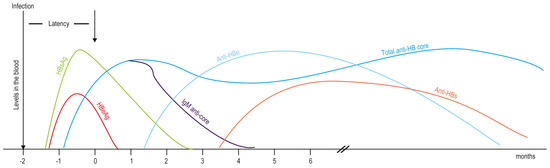
Figure 1.
Hepatitis B viral antigens and antibodies detectable in the blood following infection.
Test results can distinguish whether the patient has hepatitis B or not. Meanwhile, the Hepatitis B virus antigens and antibodies detected in the blood can also predict the therapeutic effect of antiviral drugs and immune system regulator interferon. Once chronic hepatitis B virus infection is confirmed, the patient need to do some tests to detect and measure HBV DNA. These tests are used to assess a person’s infection status and to monitor treatment [31]. Secondly, the levels of these enzymes in serum are collected in detail. The activity of enzymes in the liver is an important indicator of the liver’s function. For example, serum alanine aminotransferase (ALT) levels and aspartate transaminase (AST) levels generally reflect the degree of hepatocyte damage. Thirdly, the imaging examinations carried out, such as medical ultrasound and computed tomography. Fourth, collect the results of liver biopsy to evaluate the inflammation of the liver, exclude other liver diseases and monitor treatment. Fifth, the symptoms and medical signs, such as fatigue, abdominal distension and jaundice, are also used in the diagnosis of chronic hepatitis B. Finally, some basic pieces of information are taken into consideration, e.g., sex, age, history of drinking, history of mental illness, and medications that have been taken before. In addition, seven licensed drugs and related basic medicine for treating hepatitis B infection were introduced in the construction of the knowledge base. In fact, the information used in our diagnosis methods is basically based on objective examination results and subjective descriptions of patients. Through this information, the system can diagnose hepatitis B patients in more detail at the same time, and make a treatment plan according to their personal situation.
3.3. A Hepatitis B Diagnosis and Treatment Model Based on DUCG
Hepatitis B is a widespread epidemic disease in the world, but, up to now, there is no single drug that can kill or eliminate the hepatitis B virus and cure chronic hepatitis B virus infection. In order to give a more appropriate treatment scheme, hepatitis B infection will be further diagnosed in clinical diagnosis. Chronic hepatitis B virus infection can be divided into chronic HBV carriers, HBeAg-positive chronic hepatitis B, HBeAg-negative chronic hepatitis B, inactivity HBsAg carriers, occult chronic hepatitis B, and hepatitis B cirrhosis. We can diagnose chronic hepatitis B virus infection by detecting viral antigens and antibodies in serum, and these diseases are listed in Table 1.

Table 1.
The chronic hepatitis B virus infection subdivisions.
In order to minimize drug abuse and treat patients, different treatment plans are given for different diseases and the condition of the patient, and these treatment plans are listed in Table 2.
Table 2.
The treatment plans of chronic hepatitis B virus infection.
In the process of building the model, each disease is treated as a separate module, and some variables can be shared with other variables [27]. This is a modular modeling scheme, which allows a causal graph to be divided into semi-independent parts from multiple angles, while still keeping the consistency of events definitions. Therefore, all aspects of a disease can be described at any granularity level, and the difficulty of modeling complex system is greatly reduced. In addition, as we analyzed, incomplete knowledge and imprecise parameters have little influence on the accuracy of reasoning. These characteristics have brought us great flexibility in using statistical data and domain knowledge.
For example, Figure 2 and Figure 3 demonstrate two sub-graphs of HBeAg-positive chronic hepatitis B.
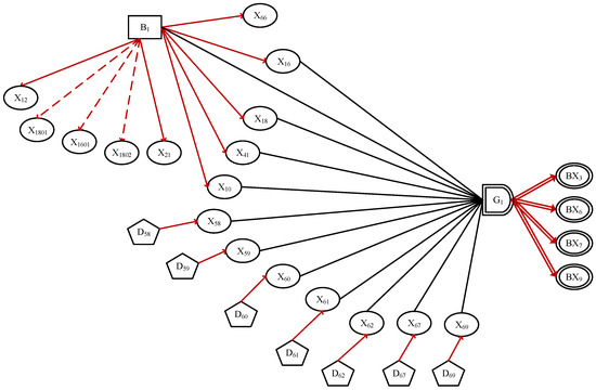
Figure 2.
The sub-DUCG includes treatment plans of HBeAg-positive chronic hepatitis B.
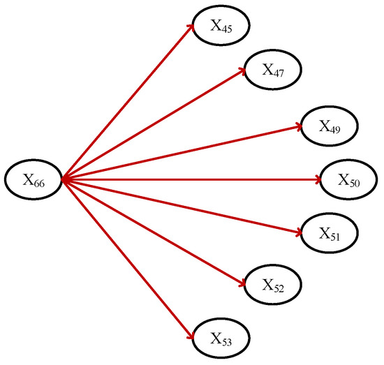
Figure 3.
The sub-DUCG includes symptoms and signs of HBeAg-positive chronic hepatitis B.
For the sake of simplicity, the variable symbols “B” and “X” are omitted from the system, and only their subscripts are kept. All causality and related parameters, such as event matrices , are decided by domain knowledge.
3.4. A Introduction to the Sub-DUCG for HBeAg-Positive Chronic Hepatitis B
Based on the prior knowledge and previous works of DUCG, after the initial diagnosis of hepatitis B, we will make a detailed distinction between hepatitis B diseases and recommend treatment options.
Take HBeAg-positive chronic hepatitis B as an example.
The hepatitis B surface antigens in serum () is positive in patients with HBeAg-positive chronic hepatitis B. At the same time, both the hepatitis B surface e antigens in serum () and the hepatitis B virus DNA () are positive. The serum alanine aminotransferase levels () of the patients are abnormal. Through the above laboratory test results, we can distinguish the development degree and type of hepatitis B disease in detail. After simply distinguishing the type of hepatitis B disease, we need to recommend a treatment plan for the patient based on the condition of the hepatitis B disease and the patient’s current test results. At this time, the simple diagnosis model needs further modification and addition.
To get more accurate results when we get relevant treatment plans, we need a continuous observation of some of the patient’s findings. This involves the problem that the state of the X variable for each inspection result will change over time.
In order to better express and reason about many times involved in the process of patient state observation and detection, in addition to the Duck variable that we have introduced in previous work, we add a variable preprocessing process here.
We keep the patient’s test results every time(). For each historical record, we subtract the state value of the current variable from the state value of the current variable, and record it as . For example, the status of a patient’s is 0 last time, and the status of is 2 this time. Therefore,
The positive and negative of can express the change trend of . After recording the patient’s test results multiple times, we can also get the changing trend of within a period. are added to obtain the sum of results in a period of time, , denoted as .
It should be noted that is not directly equal to the result of the t time test results, it is assigned a different state depending on the detection result. Because in addition to some variables directly as a numerical result, there are still some variables that cannot be directly described by numerical values. Here are two examples.
The status list of Jaundice() as shown as Table 3. The status list of ALT () as shown as Table 4, and the “ULN” in Table 4 means “upper limit of normal”.
Table 3.
The status list of Jaundice.
Table 4.
The status list of ALT.
For example, the weekly ALT value of a patient is 23.7, 49.5, and 115.3, respectively, and the patient has no symptoms of jaundice. The state of is 0; the state of is 2; the state of is 4; and the status of , , and are 0. During the period from to ,
and
It should be noted that when the state of is singular, the singular value of should be subtracted from the integral calculation. The can express the cumulative trend of , preventing abnormal test results at certain times from causing erroneous diagnosis. After the concepts of and were introduced into the DUCG model, the HBeAg-positive chronic hepatitis B patients were taken as examples, a more accurate diagnosis model is as shown in Figure 4.
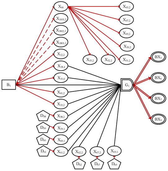
Figure 4.
The sub-graph for HBeAg-positive chronic hepatitis B.
The definitions of each X variable are shown in the Table 5.
Table 5.
The variable definitions in the sub-DUCG of HBeAg-positive chronic hepatitis B.
Antiviral therapy was used to treat HBeAg positive chronic hepatitis B. Antiviral therapy can be divided into nucleotide or nucleoside analogue therapy and interferon therapy. However, if the patient is young and the ALT value is very high ( state is more than 6), the doctor will usually observe the patient for 3 to 6 months. With a probability of 1.1% to 9%, the patient will develop antibodies to eliminate the virus and no treatment is needed. This type of treatment that requires time for continuous observation is difficult to describe in previous diagnostic models. And after introducing the and , we can clearly express this tendency. After observation, the patient did not spontaneously develop HBeAg seroconversion, and the doctor would take antiviral treatment to the patient. At the same time, after introducing the and , it is convenient to express the drug resistance process in the treatment process, to find out the drug resistance as soon as possible and replace the treatment plan. We found that in the process of causal reasoning, the diagnostic reasoning graph and the treatment reasoning graph have a certain symmetry.
4. Verification Experiments
In order to verify the effectiveness of the diagnosis and treatment system, and demonstrate the calculation details of diagnostic reasoning algorithm, we collected clinical data from patients with chronic hepatitis B. In the validation experiment, two typical cases were used as diagnostic evidence.
4.1. Verification Experiment: Case 1
In DUCG, denotes the evidence indexed by j, in which the j is a serial number of positive integers. Note that can be divided as two parts: , in which is called the abnormal evidence, is called the normal evidence.
Suppose that the evidence E collected from a patient is:
Other nonexistent X-type variables indicate that the patient is normal to the symptom, or the related pathological features are not confirmed or determined.
The purpose of the simplification is to remove the invalid or impossible causalities and irrelevant variables based on the evidence were given. In this way, the problem is more focused on, and unnecessary details are removed. Of course, the computation scale is then reduced exponentially without losing accuracy.
By applying the simplification rules to the DUCG-based diagnostic model, the irrelevant variables in the DUCG are simplified and the meaningless causal functions are removed, so as to obtain the simplified DUCG, as shown in Figure 5.
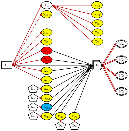
Figure 5.
The simplified DUCG in Case 1.
In order to better distinguish the states of X-type variables, ellipses of different colors is used to indicate whether a symptom are normal or not: normal state 0 is represented in green; sky blue and yellow municipal initiates state 1 and state 2; orange and red respectively indicate state 4 and state 6. And state6. Any X-type variable without color in Figure 5 means an unconfirmed/unrecognizable pathological feature. Please note that the green ellipse didn’t appear in this experiment, because all normal variables were eliminated in the process of simplifications. The simplification process is an essential step in DUCG diagnostic reasoning, and if some causal relationships lack evidentiary support, they are filtered during the simplification process and are no longer placed within the scope of the reasoning.
As we can see that Figure 5 contains all abnormal evidence, it is meaningful and explainable, and can vividly show the user how the root cause ( in this example) influenced other evidence through causal chains and led to the eventual observed symptoms.
In DCUG, assuming that only one B-type event can be true in one case. The DUCG can be decomposed as a set of sub-DUCGs k, and the weight of sub-DUCG can be calculated based on E of the sub-DUCG. Each decomposed sub-DUCG can be a further simplification. Only the sub-DUCGs which can explain are needed. And find the B-type variable of those sub-DUCGs, put them in a hypothesis space . The member in called . If there is only one member in , the diagnosis is done, because the exact result is found. The event outspread operations are first carried out to generate the hypothesis space In DUCG, assuming that only one type of event can be true in one case. The event outspread operations are first carried out to generate the hypothesis space the event outspread operations are first carried out to generate the hypothesis space . Limited by the length, we only take and as examples. The event outspread expressions are as follows.
Thus, we have
Then, we get . By ignoring all the A type events and weighing factors from the outspread expression of , we get the hypothesis space:
where indicates . Obviously, we have
Thus, the approximate state probability of conditioned on incomplete evidence is
Because of the normal evidence in Figure 5, we have
Therefore, the modification factor between and is 1, and the local state probability of is
It should be noted that is not directly equal to the result of t time test results, it is assigned a different state depending on the detection result. Because in addition to some variables directly as a numerical result, there are still some variables that cannot be directly described by numerical values. Here are two examples. The status list of Jaundice () as shown as Table 3. The status list of ALT () as shown as Table 4, and the “ULN” in Table 4 means “upper limit of normal”.
Similarly, with the above calculation, the probabilistic inference is performed in Figure 5. As we can see that Figure 5 is meaningful because it can account for all the evidence observed. The abnormal evidence is outspread as .
Thus, we have
and ( indicates ) is determined as the only candidate hypothesis of Figure 5.
We proceed to perform reasoning calculation in Figure 5, with being a candidate hypothesis, and we get that . The reasoning details are omitted for brevity.
Combining all the candidate hypotheses in the meaningful sub-DUCGs, a complete hypothesis space is obtained.
The root causes of the observed symptoms have been found without absence. After modification by a weighting coefficient associated with the prior evidence probability in each sub-DUCG containing the hypothesis , the global state probabilities of , can be obtained as
As a conclusion to this diagnostic case, these three hypotheses were identified as the possible reasons of observed evidence. And each hypothesis was able to justify itself. The probability of different states in turn indicate the possibility that the hypothesis is the root cause. and are considered more likely with larger state probabilities ( for and for ). Being exactly consistent with the doctor’s conclusion, such a quantified result can provide physicians with effective assistance in the differential diagnosis.
4.2. Verification Experiment: Case 2
Now look at another verified calculation case. It is assumed that Case 1 will undergo further clinical examination and collect more detailed medical history, while the original DUCG and parameters remain unchanged. The evidence in case 1 after supplementing the relevant symptoms is as follows.
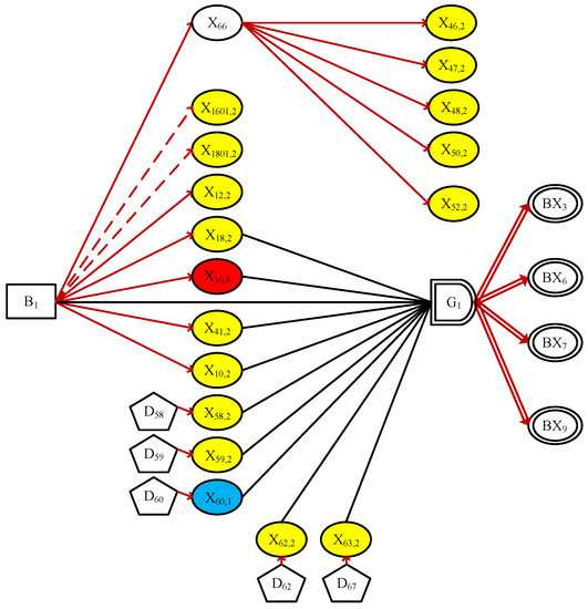
Figure 6.
The simplified DUCG in Case 2.
Note that the other two sub-DUCGs of and are both invalid and eliminated, for containing no causal explanations to some abnormal evidence such as , , , , and . Therefore, Figure 6 becomes the only meaningful sub-DUCG in this situation. The hypothesis space obtained is
where indicates . As we can see that in comparison to case 1, the more evidence observed, the smaller the hypothesis space, and the more accurate the inference result.
In fact, the root cause of the symptoms can now be determined, even if no numerical calculation is needed. Nevertheless, we complete the reasoning process in order to maintain the integrity: because of , the approximate state probability can be obtained as
Since the normal evidence , the state probability of is as expected.
In conclusion, the hypothesis is uniquely determined as the root cause of the current hepatitis B virus. This result is consistent with the clinical conclusions confirmed by doctors. The causal reasoning process can be demonstrated graphically to the user, making the conclusions and recommendations more convincing and reliable. For example, the reasoning results are shown in case 1 prove that patients with chronic hepatitis B will have better treatment results with ADV drugs in the case of LAM resistance: continuing to use LAM treatment will not achieve the desired therapeutic effect. Therefore, drug selection is not only Related to the currently diagnosed disease. Medication history also needs to be considered. Such a process of diagnostic reasoning not only produces results but also explains why the disease was proposed and why the current treatment options were chosen. Compared to its method, such probabilistic results can be explained to doctors and patients, significantly promoting clinical decisions. Besides, the system can be used as a tool for doctors to test patients’ questions and needs. Also, it can be used as an educational tool for medical students by causally mapping and visualizing certain diseases.
5. Empirical Evaluations
To evaluate the performance of the duck-based intelligent diagnosis and treatment of hepatitis B system, we randomly selected 120 cases of hepatitis B from the medical record database of Beijing Ditan Hospital. Sixty cases were selected for diagnosis and testing of hepatitis B, and 90 cases were selected for testing of treatment plan. The correct diagnosis was confirmed by doctors who are not involved in the system development. In the process of clinical diagnosis, being able to diagnosis based on incomplete information is very important for intelligent diagnosis methods. Therefore, part of the available medical evidence was discarded and used for experiments with incomplete information. Specifically, only part of the medical data is uploaded to the system, and there is no further test data. We divided the data into two groups, and detected cases with complete information and cases with incomplete information, and compared the diagnosis and treatment plan results with the confirmed correct cases. The results are as shown in Table 6.
Table 6.
The correct rate of diagnosis and treatment plan in DUCG-based system.
Remark 1.
The reason why we select only 10 cases for each disease is because most diseases have less than 10 cases. If we increase the test cases for each disease, most of the increased cases would be for only a few common diseases, which would improperly increase the precision, because the common diseases are easy to diagnose. On the other hand, 10 cases have covered most knowledge points in the DUCG and the marginal utility decreases greatly.
Remark 2.
In the actual diagnosis process, there are cases where some of the test results are missing. For example, due to financial constraints, patients did not apply for too expensive examinations. In order to simulate these conditions in the real diagnosis process, part of the information in the case has been hidden randomly. The results obtained are divided into two cases: complete medical information and incomplete medical information. Even in the case of incomplete medical information, the correct rate of the system is still acceptable. This result proves the robustness of the system to incomplete information.
The results showed that the DUCG-based system correctly diagnosed 88.3% of disease with complete information and the correct rate of the treatment plan was 95.5% with complete information.
In addition, 20 cases of non-hepatitis B were added to the test, and the system was able to diagnose 100% of non-hepatitis B patients, proving that the correct rate of the DUCG-based system for diagnosing hepatitis B disease could reach 100%. While the other methods have 74.37–98.75% correct rate when diagnosing hepatitis [32]. The comparisons are as shown in Table 7.
Table 7.
Comparisons of DUCG and other methods.
As a result, the DUCG-based intelligent diagnosis and treatment of hepatitis B system show shows high accuracy and excellent robustness. The DUCG-based method uses expressions with their own causal semantic to construct models, so that the system has the advantage of being faithful to the pathogenesis. Therefore, the conclusions obtained by the model are inherent and will not change with the application environment. This characteristic ensures the high accuracy of system diagnosis.
In addition, the error results in the test were analysed in detail. Part of them are because of the changing process of the disease samples, and the diagnosis given by the human doctors may be more conservative. Another part of the error results is caused by the inaccuracy of the relevant parameters. In this paper, the parameters in the system are given by domain experts, and may bring in some subjective factors. This leads to deviations in some of the results. One possible solution may be design a learning based parameter tuning method, to overcome the subjective bias in the parameters.
Remark 3.
The DUCG method is 100% correct. The data used is a sample of 80 cases, of which 60 cases are diagnosed with hepatitis B disease and 20 cases are non-hepatitis B disease. The DUCG method correctly diagnosed 60 cases of hepatitis B disease and ruled out another 20 cases, so the correct rate here is 100%. Of course, this result is obtained from existing case samples, and some new and different cases are also in the search process to test the diagnostic accuracy of the system under extreme conditions.
6. Conclusions and Future Work
In this study, we developed an intelligent diagnosis and treatment of hepatitis b system based on Dung, which can support the diagnosis of hepatitis b in 7 diseases and give the best treatment plan. This system includes diagnosis and treatment models, including 67 variables and 127 causal arcs. The models use clinical data(such as signs, symptoms, examination results, environmental factors, medical history, pathophysiological knowledge, and disease-related psychosocial; for causality analysis. At the same time, a modular modeling scheme is used, which enables the causality diagram to be divided into sub-graphs from multiple angles. As a result, large and complex system model are allowed to be split, and the modeling process becomes simple.
The system experiment results show that the model has good accuracy and robustness. This indicates that the system will play a role in clinical diagnosis. With the help of link reasoning and weighted logic algorithms, the system can achieve high accuracy even if the information is incomplete. In addition, the graphic representations can directly show the pathological mechanisms and express the interpretable reasoning processes. And through the graphical representation, it is also observed that the graph of the diagnostic process and the graph of the treatment process are symmetrical. This makes the diagnosis conclusions and treatment suggestions given by the system easier to accept, and helps doctors to show more objective clinical decisions to patients. The above characteristics show that this method has extensive medical significance, especially for complicated diagnosis and treatment of hepatitis B. The contributions of this paper can be concluded as:
- Introducing the expression method of the trend brought by the inspection data over time in the system;
- Providing the treatment plan after the diagnosis of the disease;
- Providing a new treatment plan immediately after the patient develops resistance to a certain drug;
- Giving an explanation of the diagnosis and treatment plan.
Of course, the current system still has certain limitations. The methods discussed in the article are mainly for the diagnosis and treatment of hepatitis B. There is not much discussion about treatment options other than interferon. In addition, the diagnosis methods used in this article are more based on the doctor’s knowledge accumulation, and there is a lack of coping methods for the existing intractable diseases that cannot be diagnosed.
As future work, we will improve the current system by integrating other diseases that cause hepatitis B. Also, the model will continue to optimize the treatment plan and try to predict the response. In addition, experiments on clinical data will continue, and test data samples will be enriched to further evaluate and improve the accuracy of the model.
Author Contributions
Conceptualization, Q.Z. and N.D.; methodology, Q.Z.; software, Q.Z. and N.D.; validation, N.D.; formal analysis, Q.Z. and N.D.; data curation, N.D.; writing—original draft preparation, N.D.; writing—review and editing, Q.Z.; funding acquisition, Q.Z. All authors have read and agreed to the published version of the manuscript.
Funding
This work was supported in part by the National Natural Science Foundation of China under Grant 61402266, Grant 61273330 and Grant 71671103.
Conflicts of Interest
The authors declare no conflict of interest. The funders had no role in the design of the study; in the collection, analyses, or interpretation of data; in the writing of the manuscript; or in the decision to publish the results.
Abbreviations
The following abbreviations are used in this manuscript.
| DUCG | Dynamic Uncertain Causality Graph |
| HBV | The hepatitis B virus |
| HBsAg | The hepatitis B surface |
| HBcAg | The hepatitis B core antigen |
| anti-HBs | antibodies to the hepatitis B surface antigen |
| anti-HBc | antibodies to the hepatitis B core antigen |
| anti-HBe | antibodies to the e antigen |
| ALT | alanine aminotransferase |
| AST | aspartate transaminase |
| IFN | Interferon alpha-2a |
| PEG | PEGylated interferon alpha-2a |
| LAM | Lamivudine |
| ADV | Adefovir Dipivoxil |
| ETV | Entecavir |
| LdT | Telbivudine |
| TDF | Tenofovir Disoprox |
Appendix A. Dynamic Uncertain Causality Graph
DUCG is a probabilistic graphical model that explicitly represents uncertain causalities among variables and performs probabilistic reasoning [24]. It is a directed graph consisting of a number of nodes (variables) and directed arcs (causalities). The main features of DUCG are:
- able to focuses on the compact representation of complex uncertain causalities;
- able to perform exact reasoning in the case of the incomplete knowledge representation;
- able to simplify the graphical knowledge base conditional on observations before numerical calculations, so that the scale and complexity of problem can be reduced exponentially; and
- much less reliant on the parameter accuracy.
An illustrative example of DUCG is shown in Figure A1.

Figure A1.
The original DUCG of the intruder detecting system.
The corresponding nodes (variables) are divided into classes as follows.
B-type variables represent the root cause variables, drawn as squares, and can only be root causes without input. Each B-type event must have a prior probability, is a basic event variable indexed by i. In Figure A1, represents rat, represents intruder, and represents earthquake.
X-type variables drawn as cycles represent the effect or consequence variables, must have at least one input and arbitrarily output. is an X-type event variable indexed by i. In Figure A1, represents infra-red, represents vibration, both and are effect variables, e.g., represents alarm, and is a consequence variable.
D-type variables are the default cause variables without input, drawn as pentagons. When a X-type variable have no reason to explain, a D-type variable are associated with the X-type variable, representing unknown causes of the X-type variable. A D-type variable can only be connected to one X-type variable, e.g., represents the default cause event variable of .
G-type variables are virtual logic gate variables. The state of G-type variable depends on the logical relationship among its parent variables (AND, OR, NOT, etc.). is a gate event variable indexed by i. In Figure A1, represents the logic gate event variable specifying the logic among and to , where the G-type variables are drawn as gates and the details of are specified in the (Logic Gate Specification i).
The A-type event encoded in a directed arc is a virtual event defined in DUCG to represent the random causality between the parent and child. The causal events A connect the parent variables and child variables. represents the effect of state j of parent variable () on state k of child variable , given that occurs, if occurs, then occurs; otherwise, does not occur.
In the event , “;” is used to separate the child variable (subscripts before) and the parent variable (subscripts after), “,” is used to separate the variable index (subscripts before) and the variable state (subscripts after), and sometimes “,” can be ignored. Usually, 0 indexes the normal state, for example, in Figure A1, the definitions of {}-type events are follows.
The probability of independent random event is . is a member of the matrix .
Define .
represents the red directed arcs among variables in DUCG. It is a with a weight coefficient. , and it represents the strength of the causal relationship between the parent variable and child variable , . is actually an event matrix with as its members.
Define .
Normal state 0 does not affect any abnormal state and it can not be caused by any abnormal state. It means that, in DUCG, the knowledge representation and casual inference can be done without specifying the cause or result of .
Probability calculation is an important part of DUCG. Posterior probability calculation of DUCG needs to expand the event expression. During the expanding, the logic operations such as AND, OR, XOR, absorption, and exclusion are used to simplify the expressions. The algorithm to expand more than one event ANDs (multiplied) together is presented in [36]. The formula of basic event expression is as follows.
In DUCG, assume , , are the parent variables of , the expression formula of event is
where j expresses the state of , represents the causal relationship intensity between and , and . is a random event that affects .
Equation (A1) can be applied repeatedly, until only B-type or D-type variables remaining. Therefore, this logical expansion can be for any X variables. In DUCG, the lower case letters represent the probabilities of the corresponding upper case letter events. Replace the upper case letters with the lower case letters in Equation (A1), we have
In addition to Figure A1, the -type variable is used in the clinical diagnosis DUCG, which is a special X-type variable and its state is to be diagnosed just like B-type events. References
References
- Obeidat, I.; Alkhasawneh, A.; Mohammad. Computer Based Clinical Decision Support System for Hepatitis Disease Diagnosis. Int. J. Adv. Comput. Technol. 2013, 5, 14–15. [Google Scholar]
- Berlin, A.; Sorani, M.; Sim, I. A taxonomic description of computer-based clinical decision support systems. J. Biomed. Inform. 2006, 39, 656–667. [Google Scholar] [CrossRef] [PubMed]
- Yardimci, A. Soft computing in medicine. Appl. Soft Comput. 2009, 9, 1029–1043. [Google Scholar] [CrossRef]
- Keith, R.D.F.; Beckley, S.; Garibaldi, J.M.; Westgate, J.A.; Ifeachor, E.C.; Greene, K.R. A multicentre comparative study of 17 experts and an intelligent computer system for managing labour using the cardiotocogram. BJOG Int. J. Obstet. Gynaecol. 1995, 102, 688–700. [Google Scholar] [CrossRef]
- Valstar, E.R.; Botha, C.P.; Glas, M.V.D.; Rozing, P.M.; Helm, F.C.T.V.D.; Post, F.H.; Vossepoel, A.M. Towards computer-assisted surgery in shoulder joint replacement. ISPRS J. Photogramm. Remote Sens. 2002, 56, 326–337. [Google Scholar] [CrossRef]
- Malek, S.; Phillips, R.; Mohsen, A.; Viant, W.; Bielby, M.; Sherman, K. Validations of Computer-Assisted Orthopaedic Surgical System for insertion of distal locking screws for intramedullary nails. Int. Congr. Ser. 2004, 1268, 614–619. [Google Scholar] [CrossRef]
- Avci, E. A New Expert System for Diagnosis of Lung Cancer: GDA—LS_SVM. J. Med. Syst. 2012, 36, 2005–2009. [Google Scholar] [CrossRef]
- Schatz, C.V.D.; Schneider, F.K. Intelligent and Expert Systems in Medicine–A Review. In Proceedings of the XVIII Congreso Argentino de Bioingenieria, Mar del Plata, Argentina, 28–30 September 2011; pp. 1–10. [Google Scholar]
- Miller, R.A.; Pople, H.E.; Myers, J.D. INTERNIST-I, An Experimental Computer-Based Diagnostic Consultant for General Internal Medicine. In Computer-Assisted Medical Decision Making; Springer: New York, NY, USA, 1985; pp. 139–158. [Google Scholar]
- Montani, S.; Bellazzi, R.; Portinale, L.; Stefanelli, M. A multi-modal reasoning methodology for managing IDDM patients. Int. J. Med. Inform. 2000, 58–59, 243–256. [Google Scholar] [CrossRef]
- Dragulescu, D.; Albu, A. Expert System for Medical Predictions. In Proceedings of the International Symposium on Applied Computational Intelligence and Informatics, Timisoara, Romania, 17–18 May 2007; pp. 123–128. [Google Scholar]
- Hsu, C.C.; Ho, C.S. A new hybrid case-based architecture for medical diagnosis. Inf. Sci. 2004, 166, 231–247. [Google Scholar] [CrossRef]
- Sun, W.; Chen, J.; Li, J. Decision tree and PCA-based fault diagnosis of rotating machinery. Mech. Syst. Signal Process. 2007, 21, 1300–1317. [Google Scholar] [CrossRef]
- Papageorgiou, E.I.; Huszka, C.; Roo, J.D.; Douali, N.; Jaulent, M.C.; Colaert, D. Application of probabilistic and fuzzy cognitive approaches in semantic web framework for medical decision support. Comput. Methods Progr. Biomed. 2013, 112, 580–598. [Google Scholar] [CrossRef] [PubMed]
- Ruffle, J.K.; Farmer, A.D.; Aziz, Q. Artificial Intelligence-Assisted Gastroenterology—Promises and Pitfalls. Am. J. Gastroenterol. 2019, 114, 422–428. [Google Scholar] [CrossRef] [PubMed]
- Erickson, B.J.; Korfiatis, P.; Kline, T.L.; Akkus, Z.; Philbrick, K.; Weston, A.D. Deep Learning in Radiology: Does One Size Fit All? J. Am. Coll. Radiol. 2018, 15, 521–526. [Google Scholar] [CrossRef]
- Yuille, A.L.; Liu, C. Deep Nets: What have they ever done for Vision? arXiv 2018, arXiv:1805.04025. [Google Scholar]
- Marcus, G. Deep Learning: A Critical Appraisal. arXiv 2018, arXiv:1801.00631. [Google Scholar]
- Shao-rui, H.; Shi-chao, G.; Lin-xiao, F.; Jia-jia, C.; Qin, Z.; Lan-juan, L. Intelligent diagnosis of jaundice with dynamic uncertain causality graph model. J. Zhejiang Univ. Sci. B (Biomed. Biotechnol.) 2016, 18, 393–401. [Google Scholar]
- Zhang, Q.; Bu, X.; Zhang, M.; Zhang, Z.; Hu, J. Dynamic uncertain causality graph for computer-aided general clinical diagnoses with nasal obstruction as an illustration. Artif. Intell. Rev. 2020. [Google Scholar] [CrossRef]
- Itani, S.; Lecron, F.; Fortemps, P. Specifics of Medical Data Mining for Diagnosis Aid: A Survey. Expert Syst. Appl. 2018, 118. [Google Scholar] [CrossRef]
- Zhou, Z.H.; Jiang, Y. Medical diagnosis with C4.5 rule preceded by artificial neural network ensemble. IEEE Trans. Inf. Technol. Biomed. 2003, 7, 37–42. [Google Scholar] [CrossRef]
- Zhang, Q.; Zhang, Z. Dynamic Uncertain Causality Graph Applied to Dynamic Fault Diagnoses and Predictions with Negative Feedbacks. IEEE Trans. Reliab. 2016, 65, 1030–1044. [Google Scholar] [CrossRef]
- Zhang, Q.; Geng, S. Dynamic Uncertain Causality Graph Applied to Dynamic Fault Diagnoses of Large and Complex Systems. IEEE Trans. Reliab. 2015, 64, 910–927. [Google Scholar] [CrossRef]
- Zhang, Q. A continuous possibility propagation diagram approach for reasoning under uncertainty. IEEE Int. Conf. Syst. 1996, 2, 1426–1429. [Google Scholar]
- Zhao, Y.; Zhang, Q.; Deng, H.C.; Dong, C.L. Application of DUCG in Fault Diagnosis of Nuclear Power Plant Secondary Loop. Yuanzineng Kexue Jishu/At. Energy Sci. Technol. 2014, 48, 496–501. [Google Scholar]
- Dong, C.; Wang, Y.; Zhang, Q.; Wang, N. The methodology of Dynamic Uncertain Causality Graph for intelligent diagnosis of vertigo. Comput. Methods Progr. Biomed. 2013, 113, 162–174. [Google Scholar] [CrossRef] [PubMed]
- Hollinger, F.B.; Lau, D.T. Hepatitis B: The pathway to recovery through treatment. Gastroenterol. Clin. N. Am. 2006, 35, 425–461. [Google Scholar] [CrossRef] [PubMed]
- Lai, C.L.; Yuen, M.F. The natural history and treatment of chronic hepatitis B: A critical evaluation of standard treatment criteria and end points. Ann. Intern. Med. 2007, 147, 58–61. [Google Scholar] [CrossRef]
- Terrault, N.A.; Bzowej, N.H.; Chang, K.M.; Hwang, J.P.; Jonas, M.M.; Murad, M.H. AASLD guidelines for treatment of chronic hepatitis B. Hepatology 2016, 63, 261. [Google Scholar] [CrossRef]
- Zoulim, F. New nucleic acid diagnostic tests in viral hepatitis. Semin. Liver Dis. 2006, 26, 309. [Google Scholar] [CrossRef]
- Afif, M.H.; Hedar, A.R.; Abdel Hamid, T.H.; Mahdy, Y.B. SS-SVM (3SVM): A New Classification Method for Hepatitis Disease Diagnosis. (IJACSA) Int. J. Adv. Comput. Sci. Appl. 2013, 4, 53. [Google Scholar]
- Bascil, M.S.; Oztekin, H. A study on hepatitis disease diagnosis using probabilistic neural network. J. Med. Syst. 2012, 36, 1603–1606. [Google Scholar] [CrossRef]
- Chen, H.L.; Liu, D.Y.; Yang, B.; Liu, J.; Wang, G. A new hybrid method based on local fisher discriminant analysis and support vector machines for hepatitis disease diagnosis. Expert Syst. Appl. Int. J. 2011, 38, 11796–11803. [Google Scholar] [CrossRef]
- Sartakhti, J.S.; Zangooei, M.H.; Mozafari, K. Hepatitis disease diagnosis using a novel hybrid method based on support vector machine and simulated annealing (SVM-SA). Comput. Methods Progr. Biomed. 2012, 108, 570–579. [Google Scholar] [CrossRef]
- Zhang, Q. Dynamic Uncertain Causality Graph for Knowledge Representation and Reasoning: Discrete DAG Cases. J. Comput. Sci. Technol. 2012, 27, 1–23. [Google Scholar] [CrossRef]
Publisher’s Note: MDPI stays neutral with regard to jurisdictional claims in published maps and institutional affiliations. |
© 2020 by the authors. Licensee MDPI, Basel, Switzerland. This article is an open access article distributed under the terms and conditions of the Creative Commons Attribution (CC BY) license (http://creativecommons.org/licenses/by/4.0/).