Article

Determination of Young’s Moduli of the Phases of Composite Materials Reinforced with Longitudinal Fibers, by Global Measurements

1
Autolive SA, B-dul Eroilor, 20, 500036 Brașov, Romania
2
Department of Mechanical Engineering, Transilvania University of Brașov, B-dul Eroilor, 20, 500036 Brașov, Romania
3
Romanian Academy of Technical Sciences, Bucharest, B-dul Dacia, 26, 030167 Bucharest, Romania
4
Farmacy, Science and Tehnology George Emil Palade of Tg, University of Medicine, 517519 Mures, Romania
*
Author to whom correspondence should be addressed.
Symmetry 2020, 12(10), 1607; https://doi.org/10.3390/sym12101607
Submission received: 11 August 2020 / Revised: 3 September 2020 / Accepted: 19 September 2020 / Published: 27 September 2020
(This article belongs to the Special Issue Composite Structures with Symmetry)

Abstract

:
The properties of a composite material are determined by the properties of the constitutive materials. In engineering practice, there are many situations in which we have composite material, but we do not have information about the properties of each phase component. The measurements we can make in such cases are on the existing material, thus being able to determine, experimentally, the global physical properties of the composite. The possibility of realizing an estimate of the mechanical properties of each component poses a problem if we start from these measurements. The paper proposes a method to achieve this, starting from the theoretical estimates established in the literature, then illustrated by an example to determine the properties of wood. Wood is a transverse isotropic material and therefore the constitutive law has symmetries that are manifested in the decrease of the number of parameters that define the stress-strain liason, defined only by five independent parameters. The proposed method can be extended to a diversity of models and materials used in the study of composite materials.

1. Introduction

Composite materials are made up of two or more phases, to finally obtain a new material with better properties, at a lower price. The properties obtained are determined by the concentration of the components, the arrangement mode, the geometry, the shape, the layout, etc. A multitude of composite materials can be obtained, and their properties can vary in an extensive range. The analysis of composite materials composed of several firmly bounded (visco) elastic materials that on a macroscopic scale can be treated as a homogeneous, isotropic/transverse isotropic or orthotropic material has long been done in the literature [1]. In general, we know the engineering constants of the materials that are put together, we know the proportion in which they appear in the composite, and we want to determine the properties of the resulting composite material. To obtain the engineering constant values of the resulting material, different methods have been applied in the literature (variational methods, boundedness methods, homogenization theory, minimum theorems, etc. [2]). Thus, sometimes very precise values of the properties of the resulting material were obtained. The literature dealing with these issues is very rich and was developed in the sixth, seventh, and eighth decades of the 20th century. However, in many cases encountered in engineering practice, there are situations in which we have a composite material, but we do not have information on the mechanical properties of its components. Measurements can be made on the existing composite material, determining, with classical methods, the values of the main engineering constants. Thus, global measurements can be made on the material, without being able to separate and determine the properties of its components. However, there are situations when knowledge of these properties becomes necessary. The problem is, therefore, that, if the values of some sizes of the composite are known measurements, it is possible to determine the values of these sizes of the composite components. The information obtained by measurements should be useful for the mechanical identification of its components.
To achieve this, appropriate theoretical models must be used that provide formulas for calculating the properties of the composite starting from the properties of its phases.
The diversity of composite materials is enormous, and that is why we will deal with the situations encountered more often in engineering, namely that of macroscopically homogeneous multiphasic linearly elastic composites, representing the classic part in the study of micromechanics of composites.
The aim of this domain is the characterizations of the macroscopic (overall) elastic behavior of the composite formed by a mixture of solid phases bounded together [2]. One of the phases is the matrix. The others are the inclusions (fibers in our study). The mixture becomes homogeneous at macroscale but is not necessary to be isotropic. Most of the studies consider the phases being too homogeneous and isotropic.
For the study that will be undertaken in this paper, it is necessary to know the relations that allow obtaining, with sufficiently good precision, the overall elastic constants of the composite material depending on the elastic constants of the composite phases. At the macroscopic level, the composite can be treated using the mechanics of continua, as a homogeneous material. From a theoretical point of view, an analysis of a composite made by different phases with different geometries to determine the elastic state of the material is a very complex task and useless for practical applications. For this reason, the problem of knowing the strain–stress in detail of a composite is replaced with the problem of the study of a statistically homogeneous composite [3,4,5]. To do this is necessary to determine the overall moduli as functions on the mechanical properties of the phases, their geometry, and other parameters that can occur.
Classical results are offered by Reuss and Voigt bound, but a rich literature presents numerous methods to compute these constants [6,7,8,9,10,11,12,13,14,15,16,17,18,19,20,21,22,23]. They can be used to determine the parameters of the phases using a set of measurements on the overall elastic parameters of the composite.
Generally, the domain of macroscopically or statistically homogeneous composite materials, has as the main subject, the characterization of the macroscopic/overall/equivalent elastic behavior of a resulting material formed by two or more solid phases bounded together. The matrix represents one of the phases, the others being the inclusions. There are no restrictions on the shape of the reinforcements materials, which may be fibrous or spherical, as an example. It is considered that the mixture is homogeneous on a macroscale, but not necessarily isotropic. Their elastic engineering constants are different, and, as a consequence, the stress and strain fields through composite become microscopically inhomogeneous [24,25,26,27,28].

2. Mathematical Method to Determine the Engineering Elastic Constants of Components Using Global Experimental Measurements

Consider a characteristic parameter of the composite that we denote by E (the most commonly used size is Young’s modulus or bulk modulus but can be shear modulus or Poisson ratio). This quantity can be expressed in terms of other unknown mechanical characteristics of the component phases x 1 , x 2 , x s and geometric known parameters p 1 , p 2 , p r :
E = g ( x 1 , x 2 , x s , p 1 , p 2 , p r ) ,   k = 1 , s ¯
The parameter considered is a parameter that can be measured. For example, in the case of Young’s modulus, a traction–compression machine can be used. Video Image Correlation is another common method used to determine other elastic constants. For this, a large number of specimens will be manufactured to perform the measurements. Let us say we made n specimens and n measurements were made. In this case, Equation (1) becomes, for each measurement:
E j = g ( x 1 , x 2 , x s , p 1 j , p 2 j , p r j ) ,   k = 1 , s ¯ ,   j = 1 , n ¯
From these measurements, we have the problem of determining a regression formula for (1), calculating the unknowns so that the last square S of the measured values from the values given by the regression function is minimum. If we denote:
S = j = 1 n [ E j g ( x 1 , x 2 , x s , p 1 j , p 2 j , p r j ) ] 2
we obtain s equations:
S x i = j = 1 n 2 [ E j g ( x 1 , x 2 , x s , p 1 j , p 2 j , p r j ) ) ] g ( x 1 , x 2 , x s , p 1 j , p 2 j , p r j ) x i = 0 ,   i = 1 , s ¯
which can be written as:
G i ( x 1 , x 2 , x s ) = 0 ,   i = 1 , s ¯
Relation (5) represents a system of s equations with s unknowns. Solving this system, we can first determine the unknowns x 1 , x 2 , x s , and we can establish the Regression Function (1) for parameter E. In this way, the unknown elastic constants of the component phases were determined. We mention that, generally, Equation (5) can be complicated, and it can be a difficult task to obtain solutions.

3. Determination of Young’s Moduli of a Multiphase Composite with Longitudinal Fibers

3.1. Using Measured Longitudinal Young’s Modulus

From a theoretical point of view, any quantity can be determined by measurements, which appears in a theoretically determined formula for any engineering constant. If the formula in which this constant appears is relatively complicated, then, of course, the necessary calculations can be particularly complicated. The system of Equation (4) can be nonlinear and sometimes difficult to solve. In these situations, it is necessary to apply specific numerical methods to solve them. However, there are also situations in which equations can be solved relatively simply. The example presented is of an important mechanical constant in engineering, Young’s modulus (longitudinal and transverse). In this case, the calculations lead to linear systems of equations that can be solved without particular difficulties. The aim is to determine Young’s modulus for constituents following the direction of the fibers and in a transverse direction. E L represents the equivalent Young’s modulus in the longitudinal direction and E T , Young’s modulus in the transverse direction. The Young’s moduli for the phases will be E m for matrix and E f 1 , E f 2 ,   , E f p for fibers ( i = 1 , p ¯ ). The percentage of the matrix in the transverse section of the specimen will be ν m , and the percentage of the fibers will be ν f 1 , ν f 2 ,   , ν f p . The obvious mathematical relationship is:
ν m + i = 1 p ν f i = 1
The well-known law of mixture offers a good estimate for Young’s modulus [1,2,3]:
E L = ν m E m + i = 1 p ν f i E f i
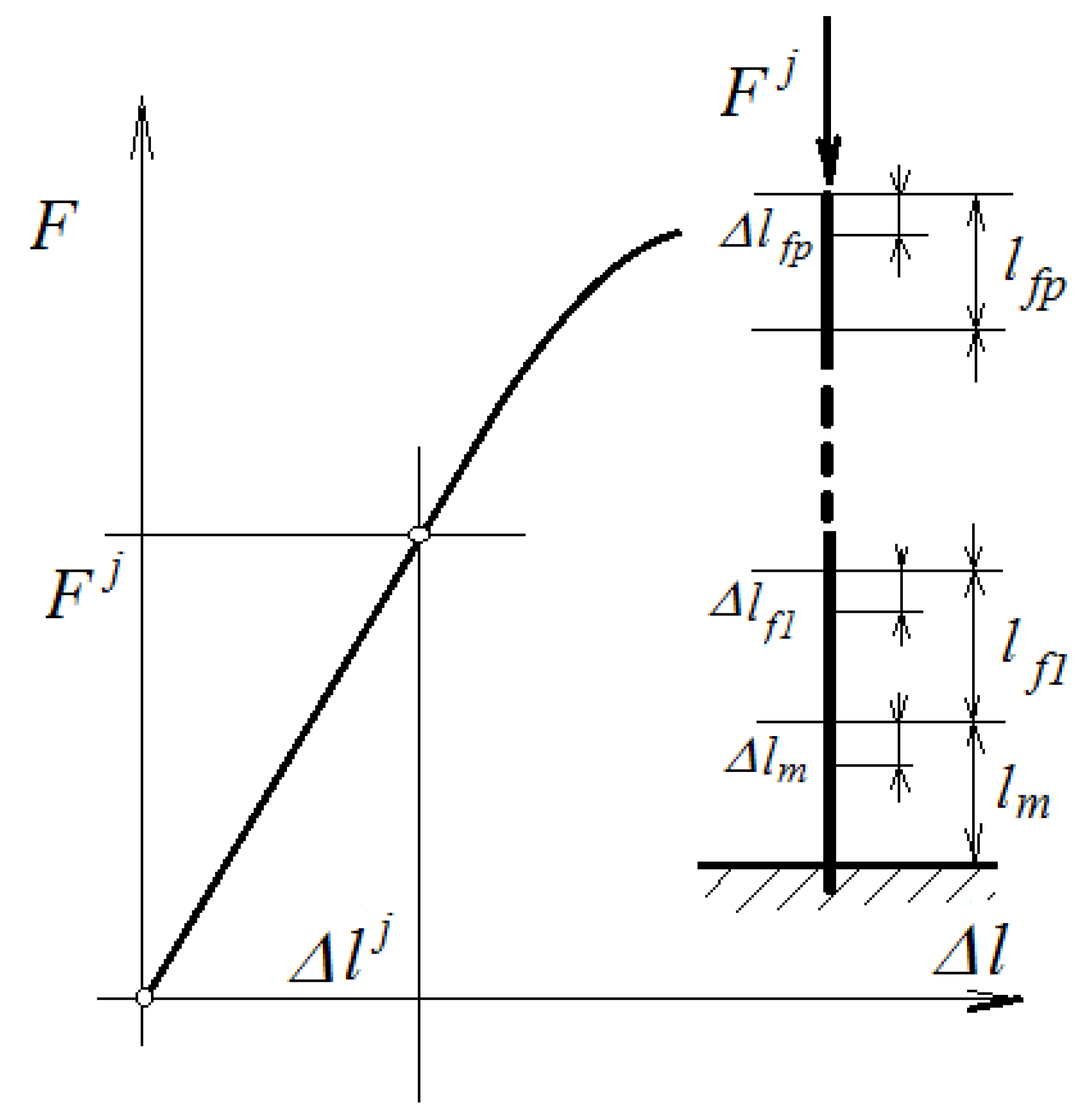
This relation will be used in further considerations. Equation (7) is justified in the following. Let us consider a set of n specimens having a known transverse area. In addition, the axis that will be used for mechanical compression is parallel to the direction of the fibers. For the studied specimen j, using the equations of static equilibrium and the Bernoulli hypothesis, the loads in the matrix and the phases ( N m j , N f 1 j , N f 2 j ,   N f p j ) from the applied load F j for these characteristic elements (Figure 1) are
{ F j = N m j + i = 1 p N f i j ; Δ l m j = Δ l f i j ;   i = 1 , p ¯ .   j = 1 , n ¯ .
The shortening of these characteristic elements, for each measurement, are
{ Δ l m j = N m j l 0 E m A m j ; Δ l f i j = N f i j l 0 E f i A f i j ;   i = 1 , p ¯ ;   j = 1 , n ¯ .
All these are equals:
Δ l m j = Δ l f 1 j = Δ l f 2 j =   Δ l f p j
The load into each phase is
{ N m j = Δ l m j l 0 E m A m j = ε m j E m A m j E m A m j N f i j = Δ l f i j l 0 E f i A f i j = ε f i j E f i A f i j = ε f i j E f i A f i j ;   i = 1 , p ¯ ;   j = 1 , n ¯ .
For the specimen j, we have
F j = N m j + i = 1 p N f i j = ε j ( E m A m j + i = 1 p E f i A f i j ) ;   j = 1 , n ¯ ,
Applying Hooke’s law for the equivalent global element, we have
F j = Δ l j l 0 E L j A j = ε j E L j A j
We have denoted the transverse aria of specimen j:
A j = A m j + A f 1 j + A f 2 j +   + A f p j ;
It results from (12) and (13):
E L j A j = E m A m j + i = 1 p E f i A f i j
If the following notations are considered:
ν m j = A m j A j ;   ν f i j = A f i j A j ;   i = 1 , p ¯ ;   j = 1 , n ¯ .
which represent the percentages of the phases from the considered specimen j. From (15) and (16), we can obtain
E L j = ν m j E m j + i = 1 p ν f i j E f i j ;   i = 1 , p ¯ ;   j = 1 , n ¯ .
The mathematical relationship (17) is the well-known law of mixtures [1,2,3]. If n measurements are made, we can obtain n relationships of this kind. The percentages of the components of the composite materials ( ν m j and ν f i j , i = 1 , p ¯ ) can be determined. We know the percentages of the volumes for the p + 1 phases and the global elasticity module measured for all n specimens, and using these values, we will determine Young’s moduli for each phase. For this, the least-squares method, previously presented, is used. Let’s consider the square of the difference:
( E L j ν m j E m i = 1 p ν f i j E f i ) 2
The objective function is:
S = j = 1 n ( E L j ν m j E m i = 1 p ν f i j E f i ) 2
and we will look for E m and E f i , i = 1 , p ¯ values, which will guarantee the minimum of the function S. These conditions for S will be expressed using these relationships:
S E m = 0 ;   S E f i = 0 ;   i = 1 , p ¯
or:
j = 1 n E L j ν m j + E m j = 1 n ( ν m j ) 2 + E f 1 j = 1 n ν m j ν f 1 j + E f 2 j = 1 n ν m j ν f 2 j   + + E f p j = 1 n ν m j   ν f p j   = 0 ; j = 1 n E L j ν f 1 j + E m j = 1 n ν f 1 j ν m j + E f 1 j = 1 n ( ν f 1 j ) 2 + E f 2 j = 1 n ν f 1 j ν f 2 j   + + E f p j = 1 n ν f 1 j ν f p j   = 0 ; j = 1 n E L j   ν f 2 j   + E m j = 1 n ν f 2 j   ν m j + E f 1 j = 1 n ν f 1 j ν f 2 j   + E f 2 j = 1 n ( ν f 2 j   ) 2 + + E f p j = 1 n ν f 2 j   ν f p j   = 0 ; j = 1 n E L j   ν f p j   + E m j = 1 n ν f p j   ν m j + E f 1 j = 1 n ν f 1 j ν f p j   + E f 2 j = 1 n ν f 2 j   ν f p j   + + E f p j = 1 n ( ν f p j   ) 2 = 0
These conditions lead to the linear system:
E m j = 1 n ( ν m j ) 2 + E f 1 j = 1 n ν m j ν f 1 j + E f 2 j = 1 n ν m j   ν f 2 j + + E f p j = 1 n ν m j   ν f p j   = j = 1 n E L j   ν m j ; E m j = 1 n ν m j   ν f 1 j + E f 1 j = 1 n ( ν f 1 j ) 2 + E f 2 j = 1 n ν f 1 j   ν f 2 j   + + E f p j = 1 n ν f 1 j   ν f p j = j = 1 n E L j ν f 1 j ; E m j = 1 n ν m j ν f p j + E f 1 j = 1 n ν f 1 j ν f p j + E f 2 j = 1 n ν f 2 j   ν f p j + + E f p j = 1 n ( ν f p j ) 2 = j = 1 n E L j ν f p j
or:
[ j = 1 n ( ν m j ) 2 j = 1 n ν m j ν f 1 j j = 1 n ν m j ν f 2 j   j = 1 n ν m j ν f p j j = 1 n ν m j   ν f 1 j j = 1 n ( ν f 1 j ) 2 j = 1 n ν f 1 j   ν f 2 j   j = 1 n ν f 1 j   ν f p j   j = 1 n ν m j   ν f p j   j = 1 n ν f 1 j   ν f p j j = 1 n ν f 2 j   ν f p j   j = 1 n ( ν f p j   ) 2 ] { E m E f 1 E f 2 E f p } = { j = 1 n E L j ν m j j = 1 n E L j   ν f 1 j j = 1 n E L j   ν f 2 j   j = 1 n E L j   ν f p j   }
having the solution:
{ E m E f 1 E f 2 E f p } = [ Q ] 1 { L }
where the notations:
[ Q ] = [ j = 1 n ( ν m j ) 2 j = 1 n ν m j   ν f 1 j j = 1 n ν m j   ν f 2 j   j = 1 n ν m j   ν f p j   j = 1 n ν m j   ν f 1 j j = 1 n ( ν f 1 j ) 2 j = 1 n ν f 1 j   ν f 2 j   j = 1 n ν f 1 j   ν f p j   j = 1 n ν m j   ν f p j   j = 1 n ν f 1 j   ν f p j   j = 1 n ν f 2 j   ν f p j   j = 1 n ( ν f p j   ) 2 ]
{ L } = { j = 1 n E L j ν m j j = 1 n E L j ν f 1 j j = 1 n E L j ν f 2 j   j = 1 n E L j ν f p j   }
were used.
The idea is to have as many measurements as possible. The higher the number of these measurements, the more accurate the obtained solution will be. The solution will be influenced by the ratio of each component and the equivalent global values of Young’s modulus. The advantage of this solution is that it uses all of the information obtained after the measurements. More measurements mean better and more exact results.

3.2. Using Measured Transverse Young’s Modulus

We have the problem of determining Young’s modulus of the composite in the direction perpendicular to the length of the fiber. Note Young’s modulus in the direction perpendicular to the global fiber (equivalent) is E T .
Consider that we have a set composed of n specimens, with a randomly cut cross-section and with the axis along which the tensile/compression stress will be applied perpendicular to the direction of the fibers (Figure 2). For the tested specimen j, there are the relations:
{ F j = N m j = N f 1 j = N f 2 j = = N f p j ; Δ l j = Δ l m j + Δ l f 1 j + Δ l f 1 j + + Δ l f p ;   j = 1 , n ¯ ; i = 1 , p ¯ ;
The shortening of these elements is:
{ Δ l m j = N m j l m j E m A = F j l m j E m A ; Δ l f 1 j = Δ l f 2 j =   = Δ l f p j = N f 1 j l f 1 j E f 1 A = N f 2 j l f 2 j E f 2 A =   = N f p j l f p j E f p A j = 1 , n ¯ ;   i = 1 , p ¯
from where we get the strain that belongs to these elements:
{ ε m j = Δ l m j l m j = N m j E m A = F j E m A ; ε f i j = Δ l f i j l f i j = N f i j E f i A = F j E f i A ,   j = 1 , n ¯ ;   i = 1 , p ¯ .
The total strain is:
ε j = Δ l j l j = Δ l m j l j + Δ l f 1 j l j + Δ l f 2 j l j + + Δ l f p l j = = Δ l m j l m j l m j l j + Δ l f 1 j l f 1 j l f 1 j l j + Δ l f 2 j l f 2 j l f 2 j l j + + Δ l f p j l f p j l f p j l j = = ε m j ν m j + ε f 1 j ν f 1 j + ε f 1 j ν f 2 j + + ε f p ν f p j ;   j = 1 , n ¯ ;   i = 1 , p ¯
where it is denoted:
ν m j = l m j l j ;   ν f 1 j = l f 1 j l j ;   ν f 2 j = l f 2 j l j ;     ;   ν f p j = l f p j l j ;   j = 1 , n ¯ ;
For the specimen j, using (29) and (30), it results:
ε j = ε m j ν m j + ε f 1 j ν f 1 j + ε f 1 j ν f 2 j + + ε f p ν f p j = = F j E m A ν m j + F j E f 1 A ν f 1 j + F j E f 2 A ν f 2 j +   + F j E f p A ν f p j = F j E T j A   j = 1 , n ¯ ;
From (27) it obtains:
1 E T j = ν m j E m + ν f 1 j E f 1 + ν f 2 j E f 2 +   + ν f p j E f p ;   j = 1 , n ¯ ;
Relation (33) is the classical form for calculating the transverse Young’s modulus [3,4,5].
If n measurements are made, then we will have n of such relations. For each measurement, the phase percentages can be determined, and the overall modulus of elasticity can be measured. The problem is, knowing the percentage volumes of the p + 1 components for each test specimen and the overall modulus of elasticity measured for all n specimens, to determine the moduli of the phases. To determine these values, the least-squares method will be applied. This is how the objective function will be built:
S = j = 1 n ( 1 E T j ν m j E m ν f 1 j E f 1 ν f 2 j E f 2   ν f p j E f p ) 2 ;
and we will look for p + 1 values E m , E f 1 , E f 2 , … E f p so that the function S is minimal. The minimum conditions for S will be expressed as
S E m = 2 j = 1 n ( 1 E T j ν m j E m ν f 1 j E f 1 ν f 2 j E f 2   ν f p , j E f p ) ν m j E m 2 = 0 ; S E f 1 = 2 j = 1 n ( 1 E T j ν m j E m ν f 1 j E f 1 ν f 2 j E f 2   ν f p , j E f p ) ν f 1 j E f 1 2 = 0 ; S E f 2 = 2 j = 1 n ( 1 E T j ν m j E m ν f 1 j E f 1 ν f 2 j E f 2   ν f p , j E f p ) ν f 2 , j E f 2 2 = 0 ; S E f p = 2 j = 1 n ( 1 E T j ν m j E m ν f 1 j E f 1 ν f 2 j E f 2   ν f p , j E f p ) ν f p , j E f p 2 = 0
Conditions (35) lead to the linear system:
1 E m j = 1 n ν m , j 2 + 1 E f 1 j = 1 n ν m j   ν f 1 j + 1 E f 2 j = 1 n ν m j   ν f 2 j +   1 E f p j = 1 n ν m j   ν f p j = j = 1 n 1 E T j ν m j ; 1 E m j = 1 n ν m j   ν f 1 j + 1 E f 1 j = 1 n ( ν f 1 j ) 2 + 1 E f 2 j = 1 n ν f 1 j ν f 2 j +   + = j = 1 n 1 E T j ν f 1 j ; 1 E m j = 1 n ν m j   ν f 2 j + 1 E f 1 j = 1 n ν f 1 j   ν f 2 j + 1 E f 2 j = 1 n ( ν f 2 j ) 2 +   + = j = 1 n 1 E T j ν f 2 j ; 1 E m j = 1 n ν m j   ν f p j + 1 E f 1 j = 1 n ν f 1 j   ν f p j + 1 E f 2 j = 1 n ν f 2 j   ν f p j +   + 1 E f p j = 1 n ( ν f p j ) 2 = j = 1 n 1 E T j ν f p j
or:
[ j = 1 n ( ν m j ) 2 j = 1 n ν m j ν f 1 j j = 1 n ν m j ν f 2 j   j = 1 n ν m j ν f p j   j = 1 n ν m j   ν f 1 j j = 1 n ( ν f 1 j ) 2 j = 1 n ν f 1 j ν f 2 j   j = 1 n ν f 1 j   ν f p j   j = 1 n ν m j   ν f p j   j = 1 n ν f 1 j   ν f p j   j = 1 n ν f 2 j   ν f p j   j = 1 n ( ν f p j   ) 2 ] { 1 E m 1 E f 1 1 E f p } = { j = 1 n ν m j E T j j = 1 n   ν f 1 j E T j j = 1 n   ν f p j E T j   }
from where:
{ 1 E m 1 E f 1 1 E f p } = [ j = 1 n ( ν m j ) 2 j = 1 n ν m j ν f 1 j j = 1 n ν m j ν f 2 j   j = 1 n ν m j ν f p j   j = 1 n ν m j   ν f 1 j j = 1 n ( ν f 1 j ) 2 j = 1 n ν f 1 j   ν f 2 j   j = 1 n ν f 1 j   ν f p j   j = 1 n ν m j   ν f p j   j = 1 n ν f 1 j   ν f p j   j = 1 n ν f 2 j   ν f p j   j = 1 n ( ν f p j   ) 2 ] 1 { j = 1 n ν m j E T j j = 1 n   ν f 1 j E T j j = 1 n   ν f p j E T j   }
which depends on the proportion of the composite phases and the overall measured values of Young’s modulus. The two elastic constants presented were analyzed for the reason that measurements could be made on wood to determine these values for early wood and late wood. Experimental verification of the proposed calculation method was thus performed.

4. Experimental Results

Wood is known to consist of two types of areas: wood formed in winter and wood formed in summer [29,30,31]. We aimed to determine the modulus of elasticity for the two types of wood. The mechanical tests were performed on wooden specimens containing both portions of summer timber and portions of winter timber, in a certain proportion, each time different for another specimen. The experimentally determined value for the transverse Young’s modulus provides an overall value for the modulus; for each test piece, we obtained a different value because the percentages of the two types of wood were different in different test specimens.
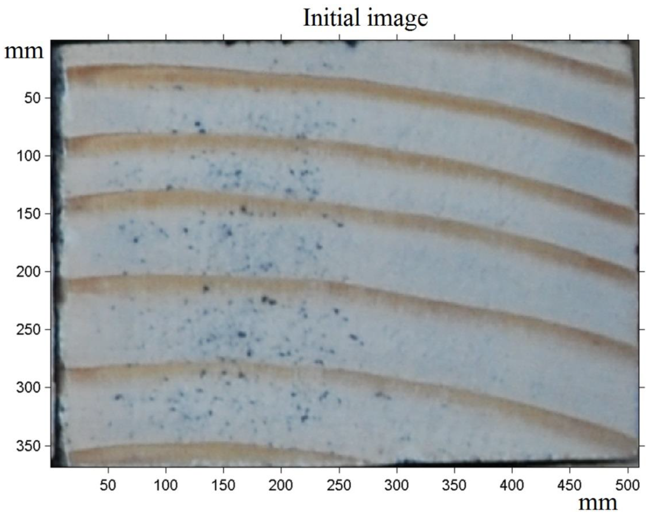
To determine the proportions of summer and winter wood, a cross-sectional image was captured and then, using specific calculation programs, the percentages of the two types of wood were determined. The picture was analyzed in the IMTOOL program (MATLAB), and the Measure Distance tool measured the number of pixels over the distance of 250 mm.
The determination of the late wood area was done through a processing program, written in MATLAB by the authors.
The first step in applying the procedure was to cut and read the picture of the section in MATLAB (Figure 3, Step 1); then, the working area of the cropped image was marked by entering the coordinate of the four corners. This was necessary because the specimens were not placed for shooting even in the normal direction of the photographic lens, and the cut-out could only be done after a rectangle. By counting the pixels in this marked area, the total area in pixels resulted (Step 2).
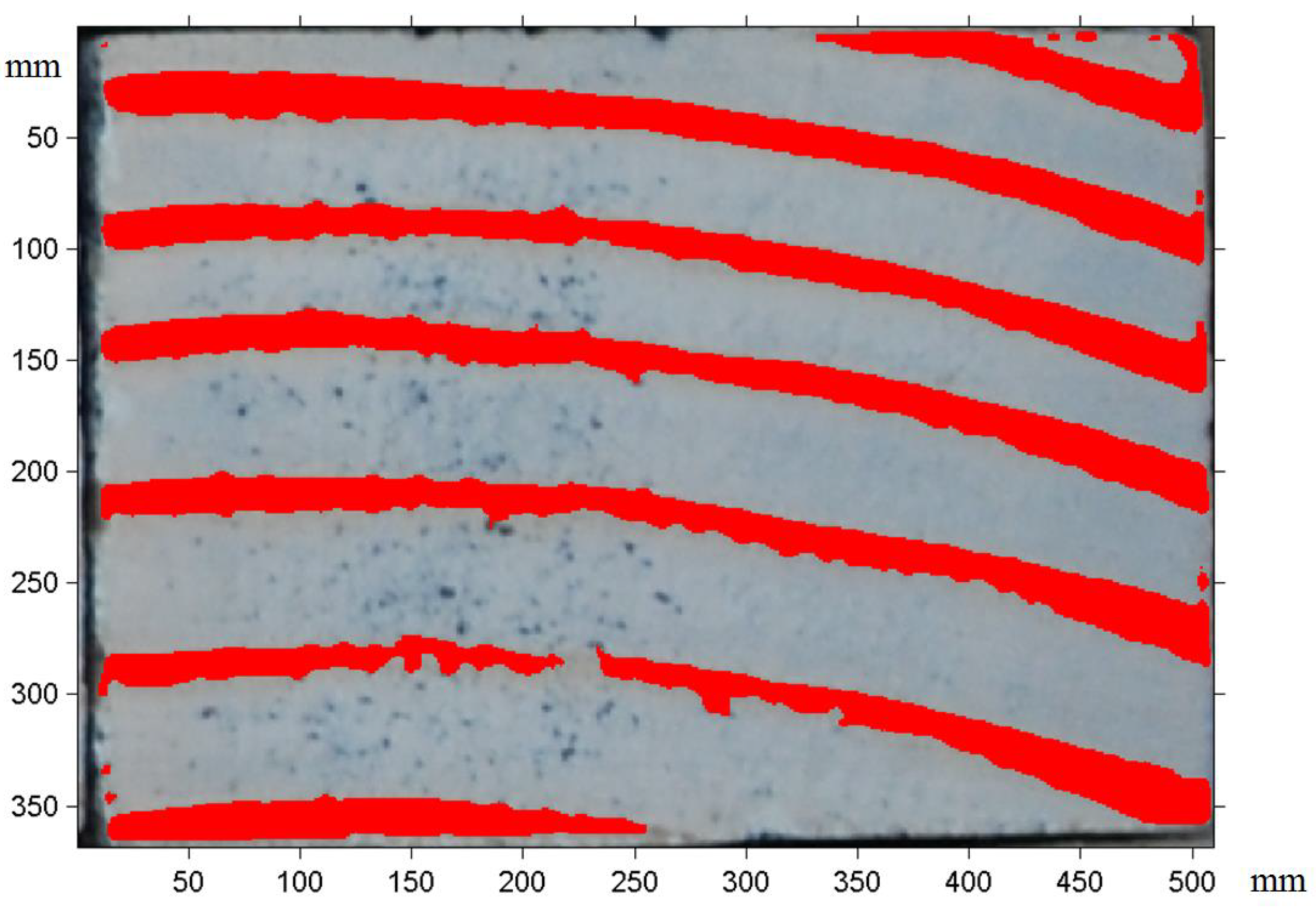
The color samples were then taken to be able to mark the late wood. This sampling was performed from one up to a maximum of five samples, until it was considered sufficient to mark areas with late wood (Steps 3.1–3.3); Step 4 was image filtering to correct any staining in areas with early wood (Figure 4).
Determining the number of pixels, which marks the late wood area, respectively, established the ratio between A / A 2 the respective A / A 1 pixels (Step 5).
To do this, we applied as an investigation method the Video Image Correlation (VIC-3D) that is a full-field one. If we considered the 3D version, this practically eliminated all disadvantages or limitations of the other experimental methods. The system consisted of two high-resolution video cameras. The setup consisted of a tripod and a high-precision connecting rod, where the cameras were fixed (see Figure 5).
Based on the mentioned procedure, each soft-wood specimen was prepared (sprayed in advance with a water-soluble paint to obtain a non-uniform dotted surface).
During the compression tests, the captured images-pairs (by the two cameras) were stored and analyzed by the VIC-3D software. In this sense, on the analyzed surface, an adequate number of points were pre-selected. The test specimens were marked by numbers (1…15).
The obtained information in displacements for each of these selected points allowed the determination of their relative displacements, respectively, and the corresponding shortening/elongations and from them, the adequate strains with a good accuracy.
During the compression tests, the force applied and the images captured by VIC-3D were correlated. Finally, one obtained the diagram F- l for a class of specimens during the loading phase, respectively, by using the adequate σ ε curves. Based on an original image analyzer program, it became possible to determine the early- and late-wood cross-sectional areas.
For example, we obtained A 1 = 364.86 mm2; A 2 = 35.14 mm2 for the specimen L 8 . As regards specimen L 6 , we obtained A 1 = 352.25 mm2; A 2 = 47.75 mm2 and A 1 = 364.86 mm2; A 2 = 35.14 mm2 were the results for specimen L 7 . The corresponding Young’s moduli for the set of 15 test specimen were as follows: E T = 2858.59 N/mm2; E L = 14,486.36 N/mm2.

5. Conclusions

In the case of measurements made on composites, they take place on the composite materials we work with. They are made up of several components and, what we measure represents the global properties of the composite as a whole. For some applications, it may be necessary to know the properties of the composite constituents. The problem then arises of how to determine these properties using measurements of engineering constants of the composite as a whole. The paper presented a method to determine, by measurements made on the composite material, the engineering constants. An application was developed to establish the individual contribution of the annual rings of the wood and their elastic properties. The advantage of this method consists in providing a better approach to the elastic properties of the individual phase. Based on the measurement strategies presented, one can determine the elastic constants of the soft-wood (for early and late rings and various types of wood material) with an acceptable accuracy provided that we carry out a representative series of statistical measurements. Accordingly, the designer has to take only the area ratio of the early and late annual rings of the wood specimen used, and they can also predict by analytical or numerical calculus the real loading capacity of that structure. The method is also valid if we have a composite made by many phases.

Author Contributions

Conceptualization, I.S. and S.V.; methodology, I.S.; software, R.I.S. and I.S.; validation, I.S., S.V. and A.M.; formal analysis, I.S. and S.V.; investigation, R.I.S. and I.S.; resources, S.V. and A.M.; data curation, R.I.S. and I.S.; writing—original draft preparation, S.V. and A.M.; writing—review and editing, I.S.; visualization, R.I.S., I.S., and S.V. and A.M.; supervision, I.S. and S.V.; project administration, I.S. and S.V.; funding acquisition, S.V. and A.M. All authors have read and agreed to the published version of the manuscript.

Funding

This research received no external funding.

Acknowledgments

We want to thank the reviewers who have read the manuscript carefully and have proposed pertinent corrections that have led to an improvement in our manuscript.

Conflicts of Interest

The authors declare no conflict of interest.

References

  1. Cristescu, N.D.; Craciun, E.M.; Soós, E. Mechanics of Elastic Composites; Chapman and Hall/CRC: London, UK, 2003. [Google Scholar]
  2. Tsai, W.; Hahn, M.T. Introduction to Composite Materials; Technomic Publishing Co.: Westport, CT, USA, 1980. [Google Scholar]
  3. Suquet, P. Matériaux Composites-Matériaux Nouveaux; Lecture Notes; University Marseille: Marseille, France, 1989. [Google Scholar]
  4. Zaoui, A. Materiaux Hétérogénes; Lecture Notes; University Marseille: Marseille, France, 1989. [Google Scholar]
  5. Garajeu, M. Contribution à L’étude du Comportement non Lineaire de Milieu Poreaux Avec ou Sans Renfort. Ph.D. Thesis, University Marseille, Marseille, France, 1995. [Google Scholar]
  6. Mandel, J. Plasticité Classique et Viscoplasticité; Courses and lectures, No. 97, Udine 1971; Springer, Wien: New York, NY, USA, 1972. [Google Scholar]
  7. Hill, R. Elastic properties of reinforced solids; some theoretical principles. J. Mech. Phys. Solids 1963, 11, 357–372. [Google Scholar] [CrossRef]
  8. Hill, R. Theory of mechanical properties of fiber-strengthened materials: I. Elastic behavior. J. Mech. Phys. Solids 1964, 12, 199–221. [Google Scholar] [CrossRef]
  9. Hill, R. Theory of mechanical properties of fiber-strengthened materials: III. Self consistent model. J. Mech. Phys. Solids 1965, 13, 189–198. [Google Scholar] [CrossRef]
  10. Hill, R. A self-consistent mechanics of composite-material. J. Mech. Phys. Solids 1965, 13, 213–222. [Google Scholar] [CrossRef]
  11. Hill, R. The essential structure of constitutive laws for metal composites and policrystals. J. Mech. Phys. Solids 1967, 15, 79–95. [Google Scholar] [CrossRef]
  12. Hill, R. On macroscopic effects of heterogeneity in elastoplastic media at finite strain. Math. Proc. Cambr. Phil. Soc. 1984, 95, 481–494. [Google Scholar] [CrossRef]
  13. Budiansky, B. On the elastic moduli of some heterogeneous materials. J. Mech. Phys. Solids 1965, 13, 223–227. [Google Scholar] [CrossRef]
  14. Hashin, Z. Theory of mechanical behavior of heterogeneous media. Appl. Mech. Rev. 1964, 17, 1–9. [Google Scholar]
  15. Hashin, Z. On the elastic behavior of fiber reinforced materials of arbitrary transverse phase geometry. J. Mech. Phys. Solids 1965, 13, 119–134. [Google Scholar] [CrossRef]
  16. Hashin, Z. Analyse of composite materials, A survey. J. Appl. Mech. 1983, 50, 481–504. [Google Scholar] [CrossRef]
  17. Hashin, Z.; Shtrikman, S. On some variational principles in anisotropic and non-homogenous elasticity. J. Mech. Phys. Solids 1962, 10, 335–342. [Google Scholar] [CrossRef]
  18. Hashin, Z.; Shtrikman, S. A variational approach to the theory of the elastic behavior of multiphase materials. J. Mech. Phys. Solids 1963, 11, 127–140. [Google Scholar] [CrossRef]
  19. Vlase, S.; Teodorescu-Draghicescu, H.; Motoc, D.L.; Scutaru, M.L.; Serbina, L.; Calin, M.R. Behavior of Multiphase Fiber-Reinforced Polymers under Short Time Cyclic Loading. Optoelectron. Adv. Mater. Rapid Commun. 2011, 5, 419–423. [Google Scholar]
  20. Teodorescu-Draghicescu, H.; Stanciu, A.; Vlase, S.; Scutaru, L.; Calin, M.R.; Serbina, L. Finite Element Method Analysis of Some Fibre-Reinforced Composite Laminates. Optoelectron. Adv. Mater. Rapid Commun. 2011, 5, 782–785. [Google Scholar]
  21. Stanciu, A.; Teodorescu-Drăghicescu, H.; Vlase, S.; Scutaru, M.L.; Călin, M.R. Mechanical behavior of CSM450 and RT800 laminates subjected to four-point bend tests. Optoelectron. Adv. Mater. Rapid Commun. 2012, 6, 495–497. [Google Scholar]
  22. Niculiță, C.; Vlase, S.; Bencze, A.; Mihălcică, M.; Calin, M.R.; Serbina, L. Optimum stacking in a multi-ply laminate used for the skin of adaptive wings. Optoelectron. Adv. Mater. Rapid Commun. 2011, 5, 1233–1236. [Google Scholar]
  23. Katouzian, M.; Vlase, S.; Calin, M.R. Experimental procedures to determine the viscoelastic parameters of laminated composites. J. Optoelectron. Adv. Mater. 2011, 13, 1185–1188. [Google Scholar]
  24. Teodorescu-Draghicescu, H.; Vlase, S.; Stanciu, M.D.; Curtu, I.; Mihalcica, M. Advanced Pultruded Glass Fibers-Reinforced Isophtalic Polyester Resin. Mater. Plast. 2015, 52, 62–64. [Google Scholar]
  25. Teodorescu-Draghicescu, H.; Scutaru, M.L.; Rosu, D.; Calin, M.R.; Grigore, P. New Advanced Sandwich Composite with twill weave carbon and EPS. J. Optoelectron. Adv. Mater. 2013, 15, 199–203. [Google Scholar]
  26. Vlase, S.; Marin, M.; Oechsner, A.; Scutaru, M.L. Motion equation for a flexible one-dimensional element used in the dynamical analysis of a multibody system. Contin. Mech. Thermodyn. 2019, 31, 715–724. [Google Scholar] [CrossRef]
  27. Abd-Elaziz, E.M.; Marin, M.; Othman, M.I. On the Effect of Thomson and Initial Stress in a Thermo-Porous Elastic Solid under G-N Electromagnetic Theory. Symmetry 2019, 11, 413. [Google Scholar] [CrossRef] [Green Version]
  28. Marin, M.; Vlase, S.; Paun, M. Considerations on double porosity structure for micropolar bodies. AIP Adv. 2015, 5, 037113. [Google Scholar] [CrossRef] [Green Version]
  29. Teodorescu-Drăghicescu, H.; Vlase, S.; Scutaru, L.; Serbina, L.; Calin, M.R. Hysteresis effect in a three-phase polymer matrix composite subjected to static cyclic loadings. Optoelectron. Adv. Mater. Rapid Commun. 2011, 5, 273–277. [Google Scholar]
  30. Bodig, J.; Jayne, B.A. Mechanics of Wood and Wood Composites; Van Nostrand Reinhold Company: New York, NY, USA, 1982. [Google Scholar]
  31. Gálfi, B.-P.; Száva, I. Experimental Method to Establish the Individual Fibres’ Mechanical Properties of the Hard-wood Specimens. In Proceedings of the 26th Symposium on Advances in Experimental Mechanics, 23–26 September 2009; Montanuniversität Leoben: Leoben, Austria, 2009; pp. 63–64. [Google Scholar]
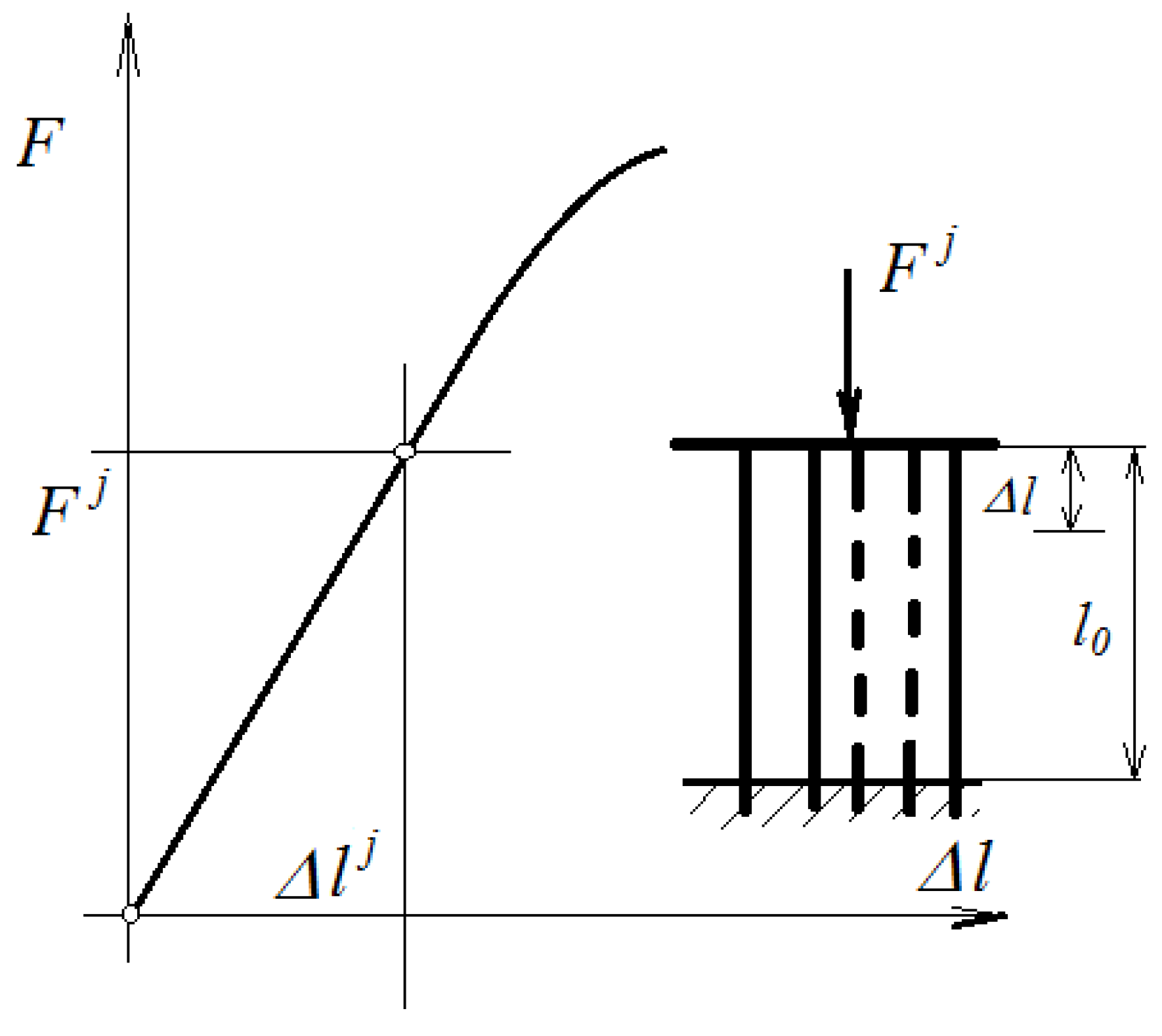
Figure 1. Longitudinal Young’s modulus.
Symmetry 12 01607 g001
Figure 2. Calculus schema for parallel-connected elements.
Symmetry 12 01607 g002
Figure 3. Capture of a cross-section. Step 1.
Symmetry 12 01607 g003
Figure 4. Step 4.
Figure 4. Step 4.
Symmetry 12 01607 g004
Figure 5. The Video Image Correlation (VIC)-3D setup.
Symmetry 12 01607 g005