Complex Patterns to the (3+1)-Dimensional B-type Kadomtsev-Petviashvili-Boussinesq Equation

Abstract

This paper presents many new complex combined dark-bright soliton solutions obtained with the help of the accurate sine-Gordon expansion method to the B-type Kadomtsev-Petviashvili-Boussinesq equation with binary power order nonlinearity. With the use of some computational programs, we plot many new surfaces of the results obtained in this paper. In addition, we present the interactions between complex travelling wave patterns and their solitons.

1. Introduction

Mathematical models named nonlinear evaluation equations (NEEs) arise in different areas of nonlinear science such as plasma physics, quantum mechanics, hydro-dynamics molecular biology, nonlinear optics, stratum water wave, optics fibers, biological science, chemistry, etc. Investigations of NEEs render possible the better understanding the complex phenomena. Recently, many new mathematical models used to describe today’s real-world problems have attracted the attention of experts from all over the world. In this sense, to observe these models some important methods such as the trial equation method, extended tanh method, modified simple equation method, extended simplest equation method, modified extended tanh method, complex method, generalized hyperbolic-function method, the homogeneous balance method, the improve F-expansion method with a Riccati equation, the improved Bernoulli sub-equation function method, the modified exponential function method and many more methods [1,2,3,4,5,6,7,8,9,10,11,12,13,14,15,16,17,18,19,20,21,22,23,24,25,26,27,28,29,30,31,32,33,34,35,36,37,38,39,40,41,42,43,44,45,46,47,48,49]. One of such models named as (3 + 1)-dimensional B-type Kadomtsev-Petviashvili-Boussinesq equation (B-type KPB) defined by

$$u_{ty}-u_{xxxy}-3{\left(u_x{u}_y\right)}_x+3u_{xz}+u_{tt}=0,$$

(1)

has been investigated [50,51]. Physically, the term $u_{tt}$ has been added and used to investigate the effect of dispersion relation and phase shift properties of the generalized B-type Kadomtsev–Petviashvili equation [51].

Y.S. Deng and his team have observed the Equation (1) via the breather-type kind soliton solutions with the help of the breather-soliton mixture [51].

In Section 2, SGEM based on fundamental equation being sine-Gordon equation Equation (1) will be defined in a detailed manner. In Section 3, some new complex combined dark-bright travelling wave solutions, which have not been studied so far to the Equation (1) will be obtained. Considering the suitable values of parameters, some graphical simulations will be also discussed. In the last section of this paper, conclusions will be presented.

2. The SGEM

Let’s consider the following sine-Gordon equation [52,53];

$$u_{xx}-u_{tt}=m^2\sin \left(u\right),$$

(2)

where $u=u\left(x,t\right),$ and $m$ is a real constant. When we apply the wave transform $u\left(x,t\right)=U\left(\xi \right), \xi =\mu \left(x-ct\right)$ to Equation (2), we obtain a nonlinear ordinary differential equation (NODE) in the form:

$$U^{″}=\frac{m^2}{{\mu }^2\left(1-c^2\right)}\sin \left(U\right),$$

(3)

where $U=U\left(\xi \right),$ and, $\xi$ is the amplitude of the travelling wave, $c$ is the velocity of the travelling wave. If we reconsider Equation (3), we can write in the full simplify version as following:

$${\left[{\left(\frac{U}{2}\right)}^{\prime }\right]}^2=\frac{m^2}{{\mu }^2\left(1-c^2\right)}{\sin }^2\left(\frac{U}{2}\right)+K,$$

(4)

where $K$ is the integration constant. When we resubmit as $K=0, w\left(\xi \right)=\frac{U}{2},$ and $a^2=\frac{m^2}{{\mu }^2\left(1-c^2\right)}$ in Equation (4), we can obtain following equation:

$$w^{\prime }=a\sin \left(w\right).$$

(5)

If we put as $a=1$ in Equation (5), we can obtain following equation:

$$w^{\prime }=\sin \left(w\right).$$

(6)

If we solve Equation (6) by using separation of variables, we find the following two significant equations:

$$\sin \left(w\right)=\sin \left(w\left(\xi \right)\right)={\frac{2p{e}^{\xi }}{p^2{e}^{2\xi }+1}|}_{p=1}=\sec h\left(\xi \right),$$

(7)

$$\cos \left(w\right)=\cos \left(w\left(\xi \right)\right)={\frac{p^2{e}^{2\xi }-1}{p^2{e}^{2\xi }+1}|}_{p=1}=\tanh \left(\xi \right),$$

(8)

where $p$ is the integral constant and non-zero. For the solution of following nonlinear partial differential equation;

$$P\left(u,u_x,u_t,\cdots \right)=0,$$

(9)

let’s consider as

$$U\left(\xi \right)={\displaystyle \sum _{i=1}^{\delta }{\tanh }^{i-1}}\left(\xi \right)\left[B_i\sec h\left(\xi \right)+A_i\tanh \left(\xi \right)\right]+A_0.$$

(10)

We can rewrite Equation (10) according to Equations (7) and (8) in the form:

$$U\left(w\right)={\displaystyle \sum _{i=1}^{\delta }{\cos }^{i-1}}\left(w\right)\left[B_i\sin \left(w\right)+A_i\cos \left(w\right)\right]+A_0.$$

(11)

Under the terms of homogenous balance technique, we can determine the values of $n$ under the terms of $NODE$. Let the coefficients of ${\sin }^i\left(w\right){\cos }^j\left(w\right)$ all be zero, it yields a system of equations. Solving this system, the values of $A_i,B_i,\mu ,c$ can be found. Finally, substituting the values of $A_i,B_i,\mu ,c$ into Equation (10), we can find the new analytical solutions to the Equation (9).

3. Application

In present part of the paper, we apply SGEM to obtain new mixed dark-bright soliton solutions to B-type KPB. Consider the following wave transformation for B-type KPB equation:

$$\mathit{u}\left(\mathit{x},\mathit{y},\mathit{t},\mathit{z}\right)=\mathit{U}\left(\mathit{\xi }\right), \mathit{\xi }=\mathit{k}\mathit{x}+\mathit{w}\mathit{y}+\mathit{r}\mathit{z}-\mathit{c}\mathit{t}.$$

(12)

This can be obtained the following differential equation:

$$\left(3\mathit{r}\mathit{k}+{\mathit{c}}^2-\mathit{c}\mathit{w}\right){\mathit{U}}^{″}-3\mathit{w}{\mathit{k}}^2{\left(\mathit{U}{\mathit{U}}^{\prime }\right)}^{\prime }-\mathit{w}{\mathit{k}}^3{\mathit{U}}^4=0.$$

(13)

Integrating Equation (12) and the constants of integrate to zero yield:

$$\left(3\mathit{r}\mathit{k}+{\mathit{c}}^2-\mathit{c}\mathit{w}\right)\mathit{U}-\frac{3\mathit{w}{\mathit{k}}^2}{2}{\mathit{U}}^2 -\mathit{w}{\mathit{k}}^3{\mathit{U}}^{″}=0.$$

(14)

Applying some simplifications, we find the following nonlinear ordinary differential equation (NODE) for B-type KPB equation:

$$2\left(3\mathit{r}\mathit{k}+{\mathit{c}}^2-\mathit{c}\mathit{w}\right)\mathit{U}-3\mathit{w}{\mathit{k}}^2{\mathit{U}}^2 -2\mathit{w}{\mathit{k}}^3{\mathit{U}}^{″}=0.$$

(15)

The homogeneous balance principle produces $n=2.$ If we consider this into Equation (11), we get the following:

$$\mathit{U}\left(\mathit{w}\right)={\mathit{B}}_1\mathbf{sin}\left(\mathit{w}\right)+{\mathit{A}}_1\mathbf{cos}\left(\mathit{w}\right)+{\mathit{B}}_2\mathbf{cos}\left(\mathit{w}\right)\mathbf{sin}\left(\mathit{w}\right)+{\mathit{A}}_2{\mathbf{cos}}^2\mathit{w}+{\mathit{A}}_0,$$

(16)

$$\begin{array}{ll}{\mathit{U}}^{″}\left(\mathit{w}\right)={\mathit{B}}_1{\mathbf{cos}}^2& \left(\mathit{w}\right)\mathbf{sin}\left(\mathit{w}\right)-{\mathit{B}}_1{\mathbf{sin}}^3\left(\mathit{w}\right)-2{\mathit{A}}_1{\mathbf{sin}}^2\left(\mathit{w}\right)\mathbf{cos}\left(\mathit{w}\right)\\ & +{\mathit{B}}_2{\mathbf{cos}}^3\left(\mathit{w}\right)\mathbf{sin}\left(\mathit{w}\right)-5{\mathit{B}}_2{\mathbf{sin}}^3\left(\mathit{w}\right)\mathbf{cos}\left(\mathit{w}\right)\\ & - 4{\mathit{A}}_2{\mathbf{cos}}^2\left(\mathit{w}\right){\mathbf{sin}}^2\left(\mathit{w}\right)+2{\mathit{A}}_2{\mathbf{sin}}^4\left(\mathit{w}\right),\end{array}$$

(17)

Substituting Equations (15) and (16) into Equation (14) produces an equation including many trigonometric terms. When we take a set of algebraic equations to zero, we find a system. Solving this system, we find the following coefficients:

Case 1 If $A_0=2k; A_1=0; A_2= -2k; B_1=0;B_2=2ik; r= \frac{-c^2+\left(c+k^3\right)w}{3k} ;$ inserting this value into Equation (10), yields the following complex combined dark-bright soliton solution:

$$\begin{array}{l}{u}_1\left(x,y,z,t\right)=2k-2ik\sec h\left[ct-kx-wy-\frac{-c^2+w\left(c+k^3\right)}{3k}z\right]\\ \times \tanh \left[ct-kx-wy-\frac{-c^2+w\left(c+k^3\right)}{3k}z\right]-2k\tanh {\left[ct-kx-wy-\frac{-c^2+w\left(c+k^3\right)}{3k}z\right]}^2,\end{array}$$

(18)

in which $c,k,w$ are real constants and non-zero. See Figure 1, Figure 2 and Figure 3 to illustrate.

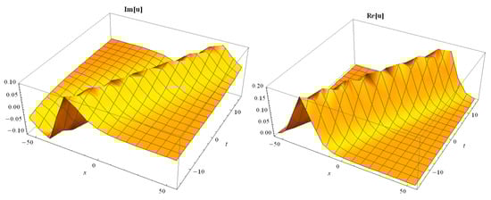
Figure 1. The 3D-dimensional surfaces of imaginary and real parts of Equation (17).

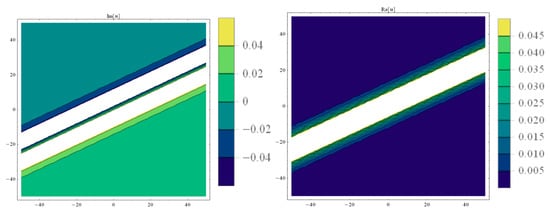
Figure 2. Contour graphs of imaginary and real parts of Equation (17).

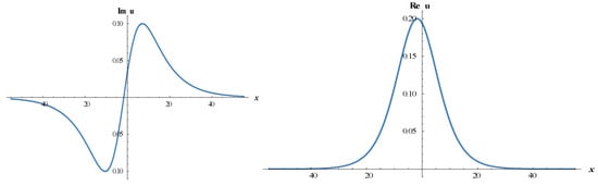
Figure 3. The 2D-dimensional surfaces of imaginary and real parts of Equation (17).

Case-2: when we choose, $A_0=\frac{4k}{3}; A_1=0; A_2= -2k; B_1=0;B_2=2ik; r= -\frac{\left(c^2-cw + k^{3}w\right)z}{3k} ;$ taking these values into Equation (10) produces another complex combined dark-bright solution to Equation (1):

$$\begin{array}{l}{u}_2\left(x,y,z,t\right)=\frac{4k}{3}-2k\tanh {\left[ct-kx-wy+\frac{c^2-cw+w{k}^3}{3k}z\right]}^2\\ +2ik\sec h\left[ct-kx-wy+\frac{c^2-cw+w{k}^3}{3k}z\right]\tanh \left[ct-kx-wy+\frac{c^2-cw+w{k}^3}{3k}z\right],\end{array}$$

(19)

where $k,c,w$ are real constants with non-zero values. Choosing the suitable values of parameters, some figures may be found as follows (see Figure 4, Figure 5, Figure 6, Figure 7, Figure 8, Figure 9, Figure 10 and Figure 11).

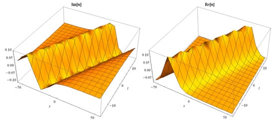
Figure 4. The 3D-dimensional surfaces of imaginary and real parts of Equation (18).

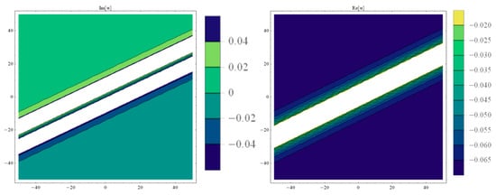
Figure 5. Contour surfaces of imaginary and real parts of Equation (18).

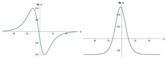
Figure 6. The 2D-dimensional surfaces of imaginary and real parts of Equation (18).

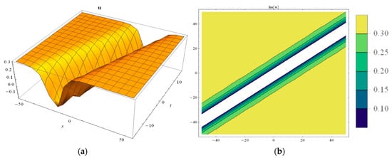
Figure 7. (a) The 3D-dimensional (left side) (b). contour surfaces of Equation (19) (right side).

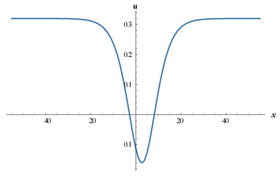
Figure 8. The 2D-dimensional surfaces of Equation (19).

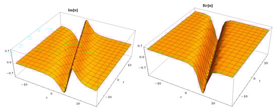
Figure 9. The 3D-dimensional surfaces of imaginary and real parts of Equation (20).

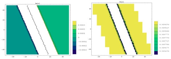
Figure 10. The contour plots of imaginary and real parts of Equation (20).

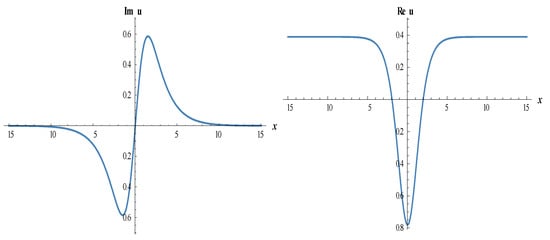
Figure 11. The 3D-dimensional surfaces of imaginary and real parts of Equation (20).

Case-3: if it is taken as for Equation (10), $A_0=\frac{4k}{3};A_1=0;A_2=-4k;B_1=0;B_2=0$ and $c=\frac{1}{2}\left(w-\sqrt{-12kr-16k^{3}w+w^2}\right)$ results in the following dark soliton solution:

$$u_3\left(x,y,t,z\right)=\frac{4k}{3}-4k\tanh {\left[-kx-wy-rz+\frac{t}{2}\left(w-\sqrt{-12kr-16k^{3}w+w^2}\right)\right]}^2,$$

(20)

in which $k,w,r$ are constants and non-zero. Some suitable values of parameters, we plot as follows:

Case-4: considering other coefficients such as $A_0=\frac{-4}{3}{c}^{\frac{1}{3}};A_1=0;A_2=2c^{\frac{1}{3}};B_1=0;B_2=-2c^{\frac{1}{3}};$ and $\mathit{k} =-{\mathit{c}}^{\frac{1}{3 }}; \mathit{w}= \frac{\mathit{c}}{2}- \frac{3\mathit{r}}{2}{\mathit{c}}^{\frac{-2}{3 }}$, for Equation (10), we find another new complex combined dark-bright solution to Equation (1) as follows:

$$\begin{array}{l}{u}_4\left(x,y,z,t\right)=\frac{-4}{3}{c}^{1/3}+2i{c}^{1/3}\sec h\left[ct+c^{1/3}x-rz-\left(\frac{c}{2}-\frac{3r}{2}{c}^{-2/3}\right)y\right]\\ \times \tanh \left[ct+c^{1/3}x-rz-\left(\frac{c}{2}-\frac{3r}{2}{c}^{-2/3}\right)y\right]+2c^{1/3}\tanh {\left[ct+c^{1/3}x-rz-\left(\frac{c}{2}-\frac{3r}{2}{c}^{-2/3}\right)y\right]}^2,\end{array}$$

(21)

with $c,r$ being real constants with non-zero values.

4. Conclusions

In this paper, we have successfully employed the SGEM to the (3 + 1)-dimensional B-type KPB equation. New dark, complex combined dark-bright soliton solutions to the governing equation have been constructed. We have observed that all solutions found in this paper have satisfied the (3 + 1)-dimensional B-type KPB equation with the help of some computational programs. To gain a better understanding of complex wave patterns, we have plotted two- and three-dimensional surfaces of the results in Figure 1, Figure 3, Figure 4, Figure 6, Figure 7a, Figure 8, Figure 9, and Figure 11 along with contour simulations given more detailed information about the low and high points of waves in a selected area Figure 2, Figure 5, Figure 7b, and Figure 10. In this sense contour simulations have become an alternative observing managing system for the results in terms of depth and height observations. Physically, dark solution, which is the third solution for Equation (19) was used to explain gravitational potential of gravity [54]. With this sense, it is estimated that these results are of such gravitational physical meanings. When we compared these results with the existing works in the literature [51], it can be observed that these solutions were of entirely new dark and complex combined dark-bright soliton solutions to the (3 + 1)-dimensional B-type KPB equation. It is estimated that the sine-Gordon equation expansion method is an efficient and powerful computational tool that can be used for studying complex nonlinear models.

Moreover, as a future work, we will investigate the stability properties of the negative solitary solutions obtained by using sine-Gordon equation expansion method in terms of orbital dynamical stability [55]. N.T. Nguyen et al. [55] have observed the orbital stability of negative solitary waves via numerical simulation by using a spectral discretization.

References

- Biswas, A.; Yıldırım, Y.; Yaşar, E.; Zhou, Q.; Moshokoa, S.P.; Belic, M. Optical soliton solutions to Fokas-Lenells equations using some different methods. Optik 2018, 173, 21–31. [Google Scholar] [CrossRef]
- Wazwaz, A.M. New (3+1)-dimensional nonlinear evolution equations with mKdV equation constituting its main part: Multiple soliton solutions. Chaos Solitons Fractals 2015, 76, 93–97. [Google Scholar] [CrossRef]
- Abdullahi, A.R. Symbolic computation on exact solutions of a coupled Kadomtsev Petviashvili equation: Lie symmetry analysis and extended tanh method. Comput. Math. Appl. 2017, 74, 1897–1902. [Google Scholar]
- Wazwaz, A.M. New travelling wave solutions to the Boussinesq and the Klein Gordon equations. Commun. Nonlinear Sci. Numer. Simul. 2008, 13, 889–901. [Google Scholar] [CrossRef]
- Wazwaz, A.M. The tanh method and the sine cosine method for solving the KP-MEW equation. Int. J. Comput. Math. 2007, 82, 235–246. [Google Scholar] [CrossRef]
- Vakhnenko, V.O.; Parkes, E.J.; Morrison, A.J. A Böcklund transformation and the inverse Scattering transform method for the generalized Vakhnenko equation. Chaos Solitons Fractals 2003, 17, 683–692. [Google Scholar] [CrossRef]
- Wazwaz, A.M. Multiple complex and multiple real soliton solutions for the integrable sine Gordon equation. Optik 2018, 172, 622–627. [Google Scholar] [CrossRef]
- Khalique, C.M.; Mhlanga, I.E. Travelling waves and conservation laws of a (2+1)-dimensional coupling system with Korteweg-de Vries equation. Appl. Math. Nonlinear Sci. 2018, 3, 241–254. [Google Scholar] [CrossRef]
- Zhao, Z.; He, L. Multiple lump solutions of the (3+1)-dimensional potential Yu-Toda-Sasa-Fukuyama equation. Appl. Math. Lett. 2019, 95, 114–121. [Google Scholar] [CrossRef]
- Tala-Tebue, E.; Tsobgni-Fozap, D.C.; Kenfack-Jiotsa, A.; Kofane, T.C. Envelope periodic solutions for a discrete network with the Jacobi elliptic functions and the alternative (G’/G)-expansion method including the generalized Riccati equation. Eur. Phys. J. Plus 2014, 129, 136. [Google Scholar] [CrossRef]
- Kudryashov, N.A.; Sinelshchikov, D.I. New non-standard Lagrangians for the Lienard-type equations. Appl. Math. Lett. 2017, 63, 124–129. [Google Scholar] [CrossRef]
- Tala-Tebue, E.; Zayed, E.M.E. New Jacobi elliptic function solutions, solitons and other solutions for the (2+1)-dimensional nonlinear electrical transmission line equation. Eur. Phys. J. Plus 2018, 133, 1–10. [Google Scholar] [CrossRef]
- Fan, E. Extended tanh-function method and its applications to nonlinear equations. Phys. Lett. A 2000, 277, 212–219. [Google Scholar] [CrossRef]
- Parkes, E.J.; Duffy, B.R. An automated tanh-function method for finding solitary wave solutions to nonlinear evolution equations. Comput. Phys. Commun. 1998, 98, 288–300. [Google Scholar] [CrossRef]
- Baskonus, H.M.; Bulut, H.; Belgacem, F.B.M. Analytical solutions for nonlinear long-short wave interaction systems with highly complex structure. J. Comput. Appl. Math. 2017, 312, 257–266. [Google Scholar] [CrossRef]
- Wazwaz, A.M. The extended tanh method for new solitons solutions for many forms of the fifth-order KdV equations. Appl. Math. Comput. 2007, 184, 1002–1014. [Google Scholar] [CrossRef]
- Qingling, G.; Xueqin, Z. A Generalized Tanh Method and its Application. Appl. Math. Sci. 2011, 5, 3789–3800. [Google Scholar]
- Whitham, G.B. Linear and Nonlinear Waves; Wiley: New York, NY, USA, 1974. [Google Scholar]
- Bulut, H.; Baskonus, H.M. On the complex structures of Kundu-Eckhaus equation via Improved Bernoulli sub-equation function method. Waves Random Complex Media 2015, 25, 720–728. [Google Scholar]
- Malfliet, W.; Hereman, W. The tanh method: II.Perturbation technique for conservative systems. Phys. Scr. 1996, 54, 569–575. [Google Scholar] [CrossRef]
- Malfliet, W. The tanh method a tool for solving certain classes of nonlinear evolution and wave equations. J. Comput. Appl. Math. 2004, 164–165, 529–541. [Google Scholar] [CrossRef]
- Wang, X.B.; Tian, S.F.; Yan, H.; Zhang, T.T. On the solitary waves, breather waves and rogue waves to a generalized (3+1)-dimensional Kadomtsev–Petviashvili equation. Comput. Math. Appl. 2017, 74, 556–563. [Google Scholar] [CrossRef]
- Gao, Y.T.; Tian, B. Generalized hyperbolic-function method with computerized Symbolic computation to construct the solitonic solutions to nonlinear equations of Mathematical physics. Comput. Phys. Commun. 2001, 133, 158–164. [Google Scholar] [CrossRef]
- Wu, X.Y.; Tian, B.; Chai, H.P.; Sun, Y. Rogue waves and lump solutions for a (3+1)-dimensional generalized B-type Kadomtsev Petviashvili equation in fluid mechanics. Mod. Phys. Lett. B 2017, 31, 1750122. [Google Scholar] [CrossRef]
- Kudryashov, N.A. A new note on exact complex travelling wave solutions for (2+1)-dimensional B-type Kadomtsev–Petviashvili equation. Appl. Math. Comput. 2010, 217, 2282–2284. [Google Scholar] [CrossRef]
- Wang, M.; Li, X.; Zhang, J. The (G’/G) expansion method and travelling wave solutions of nonlinear evolution equations in mathematical physics. Phys. Lett. A 2008, 372, 417–423. [Google Scholar] [CrossRef]
- Khalfallah, M. New Exact traveling wave solutions of the (2+1) dimensional Zakharov-Kuznetsov (ZK) equation. An. Stiintifice Ale Univ. Ovidius Constanta 2007, 15, 35–44. [Google Scholar]
- Raslan, K.R. Numerical Methods for Partial Differential Equations. Ph.D. Thesis, Al-Azhar University, Cairo, Egypt, 1999. [Google Scholar]
- Kudryashov, N.A. Traveling wave reduction of the modified KdV hierarchy: The Lax pair and the first integrals. Commun. Nonlinear Sci. Numer. Simul. 2019, 73, 472–480. [Google Scholar] [CrossRef]
- Kudryashov, N.A. Solitary and periodic waves of the hierarchy for propagation pulse in optical fiber. Optik 2019, 194, 163060. [Google Scholar] [CrossRef]
- Kudryashov, N.A. On general solutions of two nonlinear ordinary differential equations. AIP Conf. Proc. 2019, 2116, 270002. [Google Scholar]
- Zhou, Y.; Cai, S.; Liu, Q. Bounded Traveling Waves of the (2+1)-Dimensional Zoomeron Equation. Math. Probl. Eng. 2015, 163597, 1–10. [Google Scholar] [CrossRef]
- Motsepa, T.; Khalique, C.M.; Gandarias, M.L. Symmetry Analysis and Conservation Laws of the Zoomeron Equation. Symmetry 2017, 9, 27. [Google Scholar] [CrossRef]
- Liua, S.; Fu, Z.; Liu, S. Exact solutions to sine-Gordon-type equations. Phys. Lett. A 2006, 351, 59–63. [Google Scholar] [CrossRef]
- Kaur, L.; Wazwaz, A.M. Dynamical Analysis of Lump Solutions for (3+1)-dimensional generalized KP-Boussinesq equation and Its Dimensionally Reduced equations. Phys. Scr. 2018, 93, 75–203. [Google Scholar] [CrossRef]
- Cheng, L.; Zhang, Y.; Ma, W.X. Pfaffians of B-type Kadomtsev–Petviashvili equation and complexitons to a class of nonlinear partial differential equations in (3++1) dimensions. Pramana 2019, 93, 1–10. [Google Scholar] [CrossRef]
- Malfliet, W. Solitary wave solutions of nonlinear wave equations. Am. J. Phys. 1992, 60, 650–654. [Google Scholar] [CrossRef]
- Al-Amr, M.O. Exact solutions of the generalized (2 + 1)-dimensional nonlinear evolution equations via the modified simple equation method. Comput. Math. Appl. 2014, 69, 390–397. [Google Scholar] [CrossRef]
- Pandey, P.K. Solution of two point boundary value problems, a numerical approach: Parametric difference method. Appl. Math. Nonlinear Sci. 2018, 3, 649–658. [Google Scholar] [CrossRef]
- Pandey, P.K.; Jaboob, S.S.A. A finite difference method for a numerical solution of elliptic boundary value problems. Appl. Math. Nonlinear Sci. 2018, 3, 311–320. [Google Scholar] [CrossRef]
- Raslan, K.R.; Evans, D.J. The tanh function method for solving some important non-linear partial differential equations. Int. J. Comput. Math. 2005, 82, 897–905. [Google Scholar]
- Raslan, K.R.; Ali, K.K.; Shallal, M.A. The modified extended tanh method with the Riccati equation for solving the space-time fractional EW and MEW equations. Chaos Solitons Fractals 2017, 103, 404–409. [Google Scholar] [CrossRef]
- Sirendaoreji. New exact travelling wave solutions to three nonlinear evolution equations. Appl. Math. A J. Chin. Univ. 2004, 19, 178–186. [Google Scholar]
- Zhang, Y.; Pang, J. Lump and Lump-Type Solutions of the Generalized (3+1)-Dimensional Variable -Coefficient B-Type Kadomtsev-Petviashvili Equation. J. Appl. Math. 2019, 7172860, 1–10. [Google Scholar] [CrossRef]
- Cattani, C.; Sulaiman, T.A.; Baskonus, H.M.; Bulut, H. On the soliton solutions to the Nizhnik-Novikov- Veselov and the Drinfel’d-Sokolov systems. Opt. Quantum Electron. 2018, 50, 138. [Google Scholar] [CrossRef]
- Zhao, Z.; Han, B. Lump solutions of a (3+1)-dimensional B-type KP equation and its dimensionally reduced equations. Anal. Math. Phys. 2019, 9, 119–130. [Google Scholar] [CrossRef]
- Pandey, P.K. A new computational algorithm for the solution of second order initial value problems in ordinary differential equations. Appl. Math. Nonlinear Sci. 2018, 3, 167–174. [Google Scholar] [CrossRef]
- Eskitascioglu, E.I.; Aktas, M.B.; Baskonus, H.M. New Complex and Hyperbolic Forms for Ablowitz-Kaup-Newell-Segur Wave Equation with Fourth Order. Appl. Math. Nonlinear Sci. 2019, 4, 105–112. [Google Scholar]
- Baskonus, H.M.; Bulut, H.; Sulaiman, T.A. New Complex Hyperbolic Structures to the Lonngren-Wave Equation by Using Sine-Gordon Expansion Method. Appl. Math. Nonlinear Sci. 2019, 4, 141–150. [Google Scholar] [CrossRef]
- Wazwaz, A.M.; El-Tantawy, S.A. Solving the (3+1)-dimensional KP- Boussinesq and BKP-Boussinesq. Equations by the simplified Hirota’s method. Nonlinear Dyn. 2017, 88, 3017–3021. [Google Scholar] [CrossRef]
- Deng, Y.S.; Tian, B.; Sun, Y.; Zhang, C.R.; Hu, C. Rational and semi-rational solutions for the (3+1)-dimensional B-type Kadomtsev Petviashvili Boussinesq equation. Mod. Phys. Lett. B 2019, 33, 1950296. [Google Scholar] [CrossRef]
- Bulut, H.; Baskonus, H.M. New wave behaviors of the system of equations for the ion Sound and Langmuir waves. Waves Random Complex Media 2016, 26, 613–625. [Google Scholar]
- Baskonus, H.M. New acoustic wave behaviors to the Davey-Stewartson equation with power-law nonlinearity arising in fluid dynamics. Nonlinear Dyn. 2016, 86, 177–183. [Google Scholar] [CrossRef]
- Weisstein, E.W. Concise Encyclopedia of Mathematics, 2nd ed.; CRC Press: New York, NY, USA, 2002. [Google Scholar]
- Nguyen, N.T.; Kalisch, H. Orbital stability of negative solitary waves. Math. Comput. Simul. 2009, 80, 139–150. [Google Scholar] [CrossRef][Green Version]
© 2019 by the authors. Licensee MDPI, Basel, Switzerland. This article is an open access article distributed under the terms and conditions of the Creative Commons Attribution (CC BY) license (http://creativecommons.org/licenses/by/4.0/).