Use of Nonconventional Dispersion Measures to Improve the Efficiency of Ratio-Type Estimators of Variance in the Presence of Outliers

Abstract

The use of auxiliary information in survey sampling to enhance the efficiency of the estimators of population parameters is a common phenomenon. Generally, the ratio and regression estimators are developed by using the known information on conventional parameters of the auxiliary variables, such as variance, coefficient of variation, coefficient of skewness, coefficient of kurtosis, or correlation between the study and auxiliary variable. The efficiency of these estimators is dubious in the presence of outliers in the data and a nonsymmetrical population. This study presents improved variance estimators under simple random sampling without replacement with the assumption that the information on some nonconventional dispersion measures of the auxiliary variable is readily available. These auxiliary variables can be the inter-decile range, sample inter-quartile range, probability-weighted moment estimator, Gini mean difference estimator, Downton’s estimator, median absolute deviation from the median, and so forth. The algebraic expressions for the bias and mean square error of the proposed estimators are obtained and the efficiency conditions are derived to compare with the existing estimators. The percentage relative efficiencies are used to numerically compare the results of the proposed estimators with the existing estimators by using real datasets, indicating the supremacy of the suggested estimators.

1. Introduction

Suppose a finite population $W=\left\{W_1, W_2,\dots ,W_N\right\}$ consists of $N$ different and identifiable units. Let $Y$ be a measurable variable of interest with values $Y_i$ being ascertained on $W_i;i=1,2,\dots ,N$ resulting in a set of observations $Y=\left\{Y_1, Y_2,\dots ,Y_N\right\}$. The purpose of the measurement process is to estimate the population variance $S_Y^2=N^{-1}{{\displaystyle \sum }}_{i=1}^N{\left(Y_i-\overline{Y}\right)}^2$ by drawing a random sample from the population. Suppose that the information on auxiliary variable $X$ which is correlated with the study variable $Y$ is also available against every unit of the population. The use of auxiliary information to improve the efficiency of the estimators of population parameters is very popular, especially when information on the auxiliary variable is readily available and is highly correlated with the variable of interest. For instance, see [1,2,3] and the references cited therein. The ratio, product, and regression method of estimations are frequently used to enhance the efficiency of the estimators depending upon the nature of the relationship between the study and the auxiliary variables. Along with the estimation of population mean, the estimation of population variance is of importance in many real-life situations. Generally, estimation of population variance is dealt with in the context of augmenting the conventional parameters of the auxiliary variable through a ratio or regression method of estimation to achieve greater efficiency. Mostly coefficient of skewness, coefficient of kurtosis, coefficient of variation, and coefficient of correlation are used in linear combination with some other conventional parameters of the auxiliary variable to estimate the variance. The readers can refer to [4,5,6,7,8,9,10,11,12,13,14,15] and the references therein. The auxiliary measures used in most of the existing ratio-type estimators of variance are nonresistant to the presence of outliers or nonsymmetrical populations. Therefore, there is a need to develop such ratio- or regression-type estimators which are somewhat outlier resistant and more stable in the case of asymmetrical populations.

The present study is focused on estimation of population variance by incorporating information on nonconventional dispersion parameters (detailed in Section 3) of the auxiliary variable. These measures are resistant to outliers and used in a linear combination with the other conventional measures to improve the efficiency of the variance estimator under simple random sampling without replacement (SRSWOR) in the presence of outliers in the target population. The rest of the manuscript is structured as follows. The nomenclature used in the manuscript and background of the existing estimators of population variance is described in Section 2, whereas Section 3 presents the proposed improved families of estimators of population variance. In Section 4 the performance of the proposed families of the estimators is evaluated and compared with the existing estimators of population variance. Finally, some concluding remarks are given in Section 5.

2. Background of the Ratio-Type Estimators of Variance

This section deals with some of the existing estimators of population variance under simple random sampling (SRS), which utilizes the known information on conventional parameters of the auxiliary variable to enhance the efficiency of the variance estimators. Before going into the details of the existing estimators of population variance, the notation used in this manuscript is as follows.

$N$     Population size; $n$ Sample size

$f=\raisebox{1ex}{$n$}\!\left/ \!\raisebox{-1ex}{$N$}\right.$ Sampling fraction; $\eta =\frac{1-f}{n}$

$Y$     Study variable; $X$ Auxiliary variable

$\overline{Y},\overline{X}$  Population means; $\overline{y},\overline{x}$ Sample means

$S_Y,S_X$ Population standard deviations; $s_y,s_x$ Sample standard deviations

$C_Y,C_X$ Population coefficients of variation; $\rho$ Population correlation coefficient

${\beta }_{2\left(Y\right)}=\frac{{\mu }_{40}}{{\mu }_{20}^2}$ Population coefficient of kurtosis of the study variable

${\beta }_{2\left(X\right)}=\frac{{\mu }_{04}}{{\mu }_{02}^2}$ Population coefficient of kurtosis of the auxiliary variable

${\beta }_{1\left(X\right)}=\frac{{\mu }_{03}^2}{{\mu }_{02}^3}$ Population coefficient of skewness of the auxiliary variable

$M_{d\left(X\right)}$   Population median of the auxiliary variable

$Q_{1\left(X\right)}$   Population lower quartile of the auxiliary variable

$Q_{3\left(X\right)}$   Population upper quartile of the auxiliary variable

$Q_{r\left(X\right)}$   Population inter-quartile range of the auxiliary variable

$Q_{a\left(X\right)}$   Population inter-quartile average of the auxiliary variable

$Q_{d\left(X\right)}$ Population semi inter-quartile range of the auxiliary variable

$D_{i\left(X\right)}$ ith ($i=1,2,\dots ,10)$ population decile of the auxiliary variable

$B(.)$ Bias of the estimator; $MSE(.)$ Mean square error of the estimator

${\hat{S}}_R^2$  Traditional ratio estimator; ${\hat{S}}_i^2$ Existing ratio estimator

${\hat{S}}_{SK\left(i\right)}^2$   The class of estimators introduced by [16]

${\hat{S}}_{p1-j}^2$ Proposed class-I estimators; ${\hat{S}}_{p2-l}^2$ Proposed class-II estimators

${\mu }_{rs}=\frac{1}{N}{{\displaystyle \sum }}_{i=1}^N{\left(Y_i-\overline{Y}\right)}^r{\left(X_i-\overline{X}\right)}^s$; ${\lambda }_{rs}=\frac{{\mu }_{rs}}{{\mu }_{20}^{r/2}{\mu }_{02}^{s/2}}$; ${\lambda }_{22}=\frac{{\mu }_{22}}{{\mu }_{20}{\mu }_{02}}$; ${\lambda }_{21}=\frac{{\mu }_{21}}{{\mu }_{20}\sqrt{{\mu }_{02}}}$ The traditional ratio-type estimator of Isaki [4] utilizes information on the known variance $S_X^2$ of the auxiliary variable to estimate the population variance $S_Y^2$. The estimator, along with its approximate bias and MSE, is given as

$$\begin{array}{l}{\hat{S}}_R^2=\frac{s_y^2}{s_x^2}{S}_X^2,\\ B\left({\hat{S}}_R^2\right)=\eta S_Y^2\left(\left({\beta }_{2\left(X\right)}-1\right)-\left({\lambda }_{22}-1\right)\right),\\ MSE\left({\hat{S}}_R^2\right)=\eta S_Y^4 \left(\left({\beta }_{2\left(Y\right)}-1\right)+ \left({\beta }_{2\left(X\right)}-1\right)-2 \left({\lambda }_{22}-1\right)\right).\end{array}$$

(1)

Several modifications and improved estimators of variance which have been proposed in the literature make use of different conventional characteristics of the auxiliary variable. All these estimators exhibit superior efficiency as compared to the traditional ratio estimator under certain theoretical conditions. Some of the existing estimators, which utilize information on the variance of the auxiliary variable linearly integrated with other conventional parameters of the auxiliary variable, are summarized in

Table 1. Some existing estimators of variance with their bias and mean squared error.

Estimator	Proposed By	B(.)	MSE(.)
${\hat{S}}_1^2=s_y^2\left(\frac{S_X^2+{\beta }_{2\left(X\right)}}{s_x^2+{\beta }_{2\left(X\right)}}\right)$	Upadhyaya and Singh [14]	$\eta S_Y^2{\gamma }_1\left\{{\gamma }_1\left({\beta }_{2\left(X\right)}-1\right)-\left({\lambda }_{22}-1\right)\right\}$; where ${\gamma }_1=\frac{S_X^2}{S_X^2+{\beta }_{2\left(X\right)}}$	$\eta S_Y^4 \left\{\left({\beta }_{2\left(Y\right)}-1\right)+ {\gamma }_1^2\left({\beta }_{2\left(X\right)}-1\right)-2{\gamma }_1\left({\lambda }_{22}-1\right)\right\}$
${\hat{S}}_2^2=s_y^2\left(\frac{S_X^2+C_X}{s_x^2+C_X}\right)$	Kadilar and Cingi [5]	$\eta S_Y^2{\gamma }_2\left\{{\gamma }_2\left({\beta }_{2\left(X\right)}-1\right)-\left({\lambda }_{22}-1\right)\right\}$; where ${\gamma }_2=\frac{S_X^2}{S_X^2+C_X}$	$\eta S_Y^4 \left\{\left({\beta }_{2\left(Y\right)}-1\right)+ {\gamma }_2^2\left({\beta }_{2\left(X\right)}-1\right)-2{\gamma }_2\left({\lambda }_{22}-1\right)\right\}$
${\hat{S}}_3^2=s_y^2\left(\frac{S_X^2+M_{d\left(X\right)}}{s_x^2+M_{d\left(X\right)}}\right)$	Subramani and Kumarapandiyan [11]	$\eta S_Y^2{\gamma }_3\left\{{\gamma }_3\left({\beta }_{2\left(X\right)}-1\right)-\left({\lambda }_{22}-1\right)\right\}$; where ${\gamma }_3=\frac{S_X^2}{S_X^2+M_{d\left(X\right)}}$	$\eta S_Y^4 \left\{\left({\beta }_{2\left(Y\right)}-1\right)+ {\gamma }_3^2\left({\beta }_{2\left(X\right)}-1\right)-2{\gamma }_3\left({\lambda }_{22}-1\right)\right\}$
${\hat{S}}_4^2={\mathrm{s}}_{\mathrm{y}}^2\left(\frac{{\mathrm{S}}_{\mathrm{X}}^2+{\mathrm{Q}}_{1\left(\mathrm{X}\right)}}{{\mathrm{s}}_{\mathrm{x}}^2+{\mathrm{Q}}_{1\left(\mathrm{X}\right)}}\right)$	Subramani and Kumarapandiyan [13]	$\eta S_Y^2{\gamma }_4\left\{{\gamma }_4\left({\beta }_{2\left(X\right)}-1\right)-\left({\lambda }_{22}-1\right)\right\}$; where ${\gamma }_4=\frac{S_X^2}{S_X^2+Q_{1\left(X\right)}}$	$\eta S_Y^4 \left\{\left({\beta }_{2\left(Y\right)}-1\right)+ {\gamma }_4^2\left({\beta }_{2\left(X\right)}-1\right)-2{\gamma }_4\left({\lambda }_{22}-1\right)\right\}$
${\hat{S}}_5^2=s_y^2\left(\frac{S_X^2+Q_{3\left(X\right)}}{s_x^2+Q_{3\left(X\right)}}\right)$	Subramani and Kumarapandiyan [13]	$\eta S_Y^2{\gamma }_5\left\{{\gamma }_5\left({\beta }_{2\left(X\right)}-1\right)-\left({\lambda }_{22}-1\right)\right\}$; where ${\gamma }_5=\frac{S_X^2}{S_X^2+Q_{3\left(X\right)}}$	$\eta S_Y^4 \left\{\left({\beta }_{2\left(Y\right)}-1\right)+ {\gamma }_5^2\left({\beta }_{2\left(X\right)}-1\right)-2{\gamma }_5\left({\lambda }_{22}-1\right)\right\}$
${\hat{S}}_6^2=s_y^2\left(\frac{S_X^2+Q_{r\left(X\right)}}{s_x^2+Q_{r\left(X\right)}}\right)$	Subramani and Kumarapandiyan [13]	$\eta S_Y^2{\gamma }_6\left\{{\gamma }_6\left({\beta }_{2\left(X\right)}-1\right)-\left({\lambda }_{22}-1\right)\right\}$; where ${\gamma }_6=\frac{S_X^2}{S_X^2+Q_{r\left(X\right)}}$	$\eta S_Y^4 \left\{\left({\beta }_{2\left(Y\right)}-1\right)+ {\gamma }_6^2\left({\beta }_{2\left(X\right)}-1\right)-2{\gamma }_6\left({\lambda }_{22}-1\right)\right\}$
${\hat{S}}_7^2={\mathrm{s}}_{\mathrm{y}}^2\left(\frac{{\mathrm{S}}_{\mathrm{X}}^2+{\mathrm{Q}}_{\mathrm{d}\left(\mathrm{X}\right)}}{{\mathrm{s}}_{\mathrm{x}}^2+{\mathrm{Q}}_{\mathrm{d}\left(\mathrm{X}\right)}}\right)$	Subramani and Kumarapandiyan [13]	$\eta S_Y^2{\gamma }_7\left\{{\gamma }_7\left({\beta }_{2\left(X\right)}-1\right)-\left({\lambda }_{22}-1\right)\right\}$; where ${\gamma }_7=\frac{S_X^2}{S_X^2+Q_{d\left(X\right)}}$	$\eta S_Y^4 \left\{\left({\beta }_{2\left(Y\right)}-1\right)+ {\gamma }_7^2\left({\beta }_{2\left(X\right)}-1\right)-2{\gamma }_7\left({\lambda }_{22}-1\right)\right\}$
${\hat{S}}_8^2=s_y^2\left(\frac{S_X^2+Q_{a\left(X\right)}}{s_x^2+Q_{a\left(X\right)}}\right)$	Subramani and Kumarapandiyan [13]	$\eta S_Y^2{\gamma }_8\left\{{\gamma }_8\left({\beta }_{2\left(X\right)}-1\right)-\left({\lambda }_{22}-1\right)\right\}$; where ${\gamma }_8=\frac{S_X^2}{S_X^2+Q_{a\left(X\right)}}$	$\eta S_Y^4 \left\{\left({\beta }_{2\left(Y\right)}-1\right)+ {\gamma }_8^2\left({\beta }_{2\left(X\right)}-1\right)-2{\gamma }_8\left({\lambda }_{22}-1\right)\right\}$
${\hat{S}}_9^2=s_y^2\left(\frac{S_X^2+D_{1\left(X\right)}}{s_x^2+D_{1\left(X\right)}}\right)$	Subramani and Kumarapandiyan [12]	$\eta S_Y^2{\gamma }_9\left\{{\gamma }_9\left({\beta }_{2\left(X\right)}-1\right)-\left({\lambda }_{22}-1\right)\right\}$; where ${\gamma }_9=\frac{S_X^2}{S_X^2+D_{1\left(X\right)}}$	$\eta S_Y^4 \left\{\left({\beta }_{2\left(Y\right)}-1\right)+ {\gamma }_9^2\left({\beta }_{2\left(X\right)}-1\right)-2{\gamma }_9\left({\lambda }_{22}-1\right)\right\}$
${\hat{S}}_{10}^2=s_y^2\left(\frac{S_X^2+D_{2\left(X\right)}}{s_x^2+D_{2\left(X\right)}}\right)$	Subramani and Kumarapandiyan [12]	$\eta S_Y^2{\gamma }_{10}\left\{{\gamma }_{10}\left({\beta }_{2\left(X\right)}-1\right)-\left({\lambda }_{22}-1\right)\right\}$; where ${\gamma }_{10}=\frac{S_X^2}{S_X^2+D_{2\left(X\right)}}$	$\eta S_Y^4 \left\{\left({\beta }_{2\left(Y\right)}-1\right)+ {\gamma }_{10}^2\left({\beta }_{2\left(X\right)}-1\right)-2{\gamma }_{10}\left({\lambda }_{22}-1\right)\right\}$
${\hat{S}}_{11}^2=s_y^2\left(\frac{S_X^2+D_{3\left(X\right)}}{s_x^2+D_{3\left(X\right)}}\right)$	Subramani and Kumarapandiyan [12]	$\eta S_Y^2{\gamma }_{11}\left\{{\gamma }_{11}\left({\beta }_{2\left(X\right)}-1\right)-\left({\lambda }_{22}-1\right)\right\}$; where ${\gamma }_{11}=\frac{S_X^2}{S_X^2+D_{3\left(X\right)}}$	$\eta S_Y^4 \left\{\left({\beta }_{2\left(Y\right)}-1\right)+ {\gamma }_{11}^2\left({\beta }_{2\left(X\right)}-1\right)-2{\gamma }_{11}\left({\lambda }_{22}-1\right)\right\}$
${\hat{S}}_{12}^2=s_y^2\left(\frac{S_X^2+D_{4\left(X\right)}}{s_x^2+D_{4\left(X\right)}}\right)$	Subramani and Kumarapandiyan [12]	$\eta S_Y^2{\gamma }_{12}\left\{{\gamma }_{12}\left({\beta }_{2\left(X\right)}-1\right)-\left({\lambda }_{22}-1\right)\right\}$; where ${\gamma }_{12}=\frac{S_X^2}{S_X^2+D_{4\left(X\right)}}$	$\eta S_Y^4 \left\{\left({\beta }_{2\left(Y\right)}-1\right)+ {\gamma }_{12}^2\left({\beta }_{2\left(X\right)}-1\right)-2{\gamma }_{12}\left({\lambda }_{22}-1\right)\right\}$
${\hat{S}}_{13}^2=s_y^2\left(\frac{S_X^2+D_{5\left(X\right)}}{s_x^2+D_{5\left(X\right)}}\right)$	Subramani and Kumarapandiyan [12]	$\eta S_Y^2{\gamma }_{13}\left\{{\gamma }_{13}\left({\beta }_{2\left(X\right)}-1\right)-\left({\lambda }_{22}-1\right)\right\}$; where ${\gamma }_{13}=\frac{S_X^2}{S_X^2+D_{5\left(X\right)}}$	$\eta S_Y^4 \left\{\left({\beta }_{2\left(Y\right)}-1\right)+ {\gamma }_{13}^2\left({\beta }_{2\left(X\right)}-1\right)-2{\gamma }_{13}\left({\lambda }_{22}-1\right)\right\}$
${\hat{S}}_{14}^2=s_y^2\left(\frac{S_X^2+D_{6\left(X\right)}}{s_x^2+D_{6\left(X\right)}}\right)$	Subramani and Kumarapandiyan [12]	$\eta S_Y^2{\gamma }_{14}\left\{{\gamma }_{14}\left({\beta }_{2\left(X\right)}-1\right)-\left({\lambda }_{22}-1\right)\right\}$; where ${\gamma }_{14}=\frac{S_X^2}{S_X^2+D_{6\left(X\right)}}$	$\eta S_Y^4 \left\{\left({\beta }_{2\left(Y\right)}-1\right)+ {\gamma }_{14}^2\left({\beta }_{2\left(X\right)}-1\right)-2{\gamma }_{14}\left({\lambda }_{22}-1\right)\right\}$
${\hat{S}}_{15}^2=s_y^2\left(\frac{S_X^2+D_{7\left(X\right)}}{s_x^2+D_{7\left(X\right)}}\right)$	Subramani and Kumarapandiyan [12]	$\eta S_Y^2{\gamma }_{15}\left\{{\gamma }_{15}\left({\beta }_{2\left(X\right)}-1\right)-\left({\lambda }_{22}-1\right)\right\}$; where ${\hat{S}}_{15}^2=s_y^2\left(\frac{S_X^2+D_{7\left(X\right)}}{s_x^2+D_{7\left(X\right)}}\right)$	$\eta S_Y^4 \left\{\left({\beta }_{2\left(Y\right)}-1\right)+ {\gamma }_{15}^2\left({\beta }_{2\left(X\right)}-1\right)-2{\gamma }_{15}\left({\lambda }_{22}-1\right)\right\}$
	Subramani and Kumarapandiyan [12]	$\eta S_Y^2{\gamma }_{16}\left\{{\gamma }_{16}\left({\beta }_{2\left(X\right)}-1\right)-\left({\lambda }_{22}-1\right)\right\}$; where ${\gamma }_{16}=\frac{S_X^2}{S_X^2+D_{8\left(X\right)}}$	$\eta S_Y^4 \left\{\left({\beta }_{2\left(Y\right)}-1\right)+ {\gamma }_{16}^2\left({\beta }_{2\left(X\right)}-1\right)-2{\gamma }_{16}\left({\lambda }_{22}-1\right)\right\}$
${\hat{S}}_{17}^2=s_y^2\left(\frac{S_X^2+D_{9\left(X\right)}}{s_x^2+D_{9\left(X\right)}}\right)$	Subramani and Kumarapandiyan [12]	$\eta S_Y^2{\gamma }_{17}\left\{{\gamma }_{17}\left({\beta }_{2\left(X\right)}-1\right)-\left({\lambda }_{22}-1\right)\right\}$; where ${\gamma }_{17}=\frac{S_X^2}{S_X^2+D_{9\left(X\right)}}$	$\eta S_Y^4 \left\{\left({\beta }_{2\left(Y\right)}-1\right)+ {\gamma }_{17}^2\left({\beta }_{2\left(X\right)}-1\right)-2{\gamma }_{17}\left({\lambda }_{22}-1\right)\right\}$
${\hat{S}}_{18}^2=s_y^2\left(\frac{S_X^2+D_{10\left(X\right)}}{s_x^2+D_{10\left(X\right)}}\right)$	Subramani and Kumarapandiyan [12]	$\eta S_Y^2{\gamma }_{18}\left\{{\gamma }_{18}\left({\beta }_{2\left(X\right)}-1\right)-\left({\lambda }_{22}-1\right)\right\}$; where ${\gamma }_{18}=\frac{S_X^2}{S_X^2+D_{10\left(X\right)}}$	$\eta S_Y^4 \left\{\left({\beta }_{2\left(Y\right)}-1\right)+ {\gamma }_{18}^2\left({\beta }_{2\left(X\right)}-1\right)-2{\gamma }_{18}\left({\lambda }_{22}-1\right)\right\}$
${\hat{S}}_{19}^2=s_y^2\left(\frac{C_X{S}_X^2+{\beta }_{2\left(X\right)}}{C_X{s}_x^2+{\beta }_{2\left(X\right)}}\right)$	Kadilar and Cingi [5]	$\eta S_Y^2{\gamma }_{19}\left\{{\gamma }_{19}\left({\beta }_{2\left(X\right)}-1\right)-\left({\lambda }_{22}-1\right)\right\}$; where ${\gamma }_{19}=\frac{C_X{S}_X^2}{C_X{S}_X^2+{\beta }_{2\left(X\right)}}$	$\eta S_Y^4 \left\{\left({\beta }_{2\left(Y\right)}-1\right)+ {\gamma }_{19}^2\left({\beta }_{2\left(X\right)}-1\right)-2{\gamma }_{19}\left({\lambda }_{22}-1\right)\right\}$
${\hat{S}}_{20}^2=s_y^2\left(\frac{{\beta }_{2\left(X\right)}{S}_X^2+C_X}{{\beta }_{2\left(X\right)}{s}_x^2+C_X}\right)$	Kadilar and Cingi [5]	$\eta S_Y^2{\gamma }_{20}\left\{{\gamma }_{20}\left({\beta }_{2\left(X\right)}-1\right)-\left({\lambda }_{22}-1\right)\right\}$; where ${\gamma }_{20}=\frac{{\beta }_{2\left(X\right)}{S}_X^2}{{\beta }_{2\left(X\right)}{S}_X^2+C_X}$	$\eta S_Y^4 \left\{\left({\beta }_{2\left(Y\right)}-1\right)+ {\gamma }_{20}^2\left({\beta }_{2\left(X\right)}-1\right)-2{\gamma }_{20}\left({\lambda }_{22}-1\right)\right\}$
${\hat{S}}_{21}^2 =s_y^2\left(\frac{C_X{S}_X^2+M_{d\left(X\right)}}{C_X{s}_x^2+M_{d\left(X\right)}}\right)$	Subramani and Kumarapandiyan [17]	$\eta S_Y^2{\gamma }_{21}\left\{{\gamma }_{21}\left({\beta }_{2\left(X\right)}-1\right)-\left({\lambda }_{22}-1\right)\right\}$; where ${\gamma }_{21}=\frac{C_X{S}_X^2}{C_X{S}_X^2+M_{d\left(X\right)}}$	$\eta S_Y^4 \left\{\left({\beta }_{2\left(Y\right)}-1\right)+ {\gamma }_{21}^2\left({\beta }_{2\left(X\right)}-1\right)-2{\gamma }_{21}\left({\lambda }_{22}-1\right)\right\}$
${\hat{S}}_{22}^2=s_y^2\left(\frac{\rho S_X^2+Q_{3\left(X\right)}}{\rho s_x^2+Q_{3\left(X\right)}}\right)$	Khan and Shabbir [6]	$\eta S_Y^2{\gamma }_{22}\left\{{\gamma }_{22}\left({\beta }_{2\left(X\right)}-1\right)-\left({\lambda }_{22}-1\right)\right\}$; where ${\gamma }_{22}=\frac{\rho S_X^2}{\rho S_X^2+Q_{3\left(X\right)}}$	$\eta S_Y^4 \left\{\left({\beta }_{2\left(Y\right)}-1\right)+ {\gamma }_{22}^2\left({\beta }_{2\left(X\right)}-1\right)-2{\gamma }_{22}\left({\lambda }_{22}-1\right)\right\}$
${\hat{S}}_{23}^2=s_y^2\frac{\overline{X}}{\overline{x}}$	Upadhyaya and Singh [18]	$B\left({\hat{S}}_{23}^2\right)=\eta S_Y^2\left(C_X^2-{\lambda }_{21}{C}_X\right)$	$MSE\left({\hat{S}}_{23}^2\right)=\eta S_Y^4 \left\{\left({\beta }_{2\left(Y\right)}-1\right)+ C_X^2-2 {\lambda }_{21}{C}_X\right\}$

with their respective bias, MSEs, and constants.

Recently Subramani and Kumarapandiyan [16] proposed a new class of modified ratio-type estimators of population variance by modifying the estimator proposed by Upadhyaya and Singh [17]. They showed that their new class of estimators outperforms the estimators suggested in [5,11,12,13,14,17,18] under certain conditions.

The general structure of the Subramani and Kumarapandiyan [16] class of estimators is given as

$$\begin{array}{l}{\hat{S}}_{SK\left(i\right)}^2=s_y^2\left(\frac{\overline{X}+{\omega }_i}{\overline{x}+{\omega }_i}\right);i=1,2,\dots ,51\\ B\left({\hat{S}}_{SK\left(i\right)}^2\right)=\eta S_Y^2\left\{{\gamma }_{SK\left(i\right)}^2{C}_X^2-{\gamma }_{SK\left(i\right)}{\lambda }_{21}{C}_X\right\}; where {\gamma }_{SK\left(i\right)}=\frac{\overline{X}}{\overline{X}+{\omega }_i} \end{array}$$

(2)

$$MSE\left({\hat{S}}_{SK\left(i\right)}^2\right)=\eta S_Y^4 \left\{\left({\beta }_{2\left(Y\right)}-1\right)+ {\gamma }_{SK\left(i\right)}^2{C}_X^2-2{\gamma }_{SK\left(i\right)}{\lambda }_{21}{C}_X\right\}$$

(3)

where ${\omega }_i$, $i=1,2,\dots , 51$ are different choices of parameters of the auxiliary variable $X$ which can be found in Appendix A.

All these estimators exhibit superior efficiency as compared to the traditional ratio-type estimators suggested by Isaki [4] under certain conditions, but most of these estimators are based on conventional parameters of the auxiliary variable. Although many other estimators of variance are available in the existing literature, they are more complex and involve laborious computational details. Therefore, the above detailed estimators were chosen for comparison purposes due to the simplicity of their structure and relatively lower computational complexities for practitioners.

3. Proposed Estimators of Variance

This section presents two different families of ratio estimators of population variance for the case where information on some nonconventional measures of dispersion of the auxiliary variable is readily available. The nonconventional measures used to develop the new ratio estimators of variance include the following.

• Inter-decile Range: The inter-decile range is the difference between the largest decile $D_{9\left(X\right)}$ and smallest decile $D_{1\left(X\right)}$. Symbolically it is given as

  $$ID{R}_X=D_{9\left(X\right)}-D_{1\left(X\right)}$$
• Sample Inter-quartile Range: The sample inter-quartile range is based on the difference between the upper $Q_{3\left(X\right)}$ and lower $Q_{1\left(X\right)}$ quartiles as discussed by Riaz [19] and Nazir et al. [20]. It is computed as

  $$SIQ{R}_X=\frac{Q_{3\left(X\right)}-Q_{1\left(X\right)}}{1.34898}$$

  .
• Probability Weighted Moment Estimator: The probability weighted moment estimator of dispersion suggested by Downton [21] is based on the ordered sample statistics and it is defined as

  $$SP{W}_X=\frac{\sqrt{\pi }}{N^2}{{\displaystyle \sum }}_{i=1}^N\left(2i-N-1\right)X_{\left(i\right)},$$

  where $X_{\left(i\right)}$ denotes the $i$th order sample statistics.
• Downton’s Estimator: Another estimator of dispersion, similar to $SP{W}_X$, was proposed by Downton [21] and defined as

  $$DO{W}_X=\frac{2\sqrt{\pi }}{N\left(N-1\right)}{{\displaystyle \sum }}_{i=1}^N\left(i-\frac{N+1}{2}\right)X_{\left(i\right)}.$$
• Gini Mean Difference Estimator: Gini [22] introduced a dispersion estimator which is also based on the sample order statistics. It is given as

  $$G_X=\frac{4}{N-1}{{\displaystyle \sum }}_{i=1}^N\left(\frac{2i-N-1}{2N}\right)X_{\left(i\right)}.$$
• Median Absolute Deviation from Median: Hampel [23] suggested an estimator of dispersion based on absolute deviation from the median. It is defined as

  $$MAD{M}_X=1.4826\left[median\left|X_i-\tilde{X}\right|\right]$$

  , where $\tilde{X}$ is the median.
• The Median of Pairwise Distances: Shamos [24] (p. 260) and Bickel and Lehmann [25] (p. 38) suggested an estimator of dispersion which is based on the median of pairwise distances as $\left[median\left|X_i-X_l\right|;i<l\right]$. Rousseeuw and Croux [26] suggested to pre-multiply it by 1.0483 to achieve consistency under the Gaussian distribution, and the resultant estimator can be defined as

  $$B{n}_X=1.0483\left[median\left|X_i-X_l\right|;i<l\right]$$

  .
• Median Absolute Deviation from Mean: Wu et al. [27] defined another estimator which is also based on absolute deviation from the mean. It is given as

  $$MA{D}_X=median\left|X_i-\overline{X}\right|.$$
• Mean Absolute Deviation from Mean: Wu et al. [27] suggested an estimator of dispersion which is based on absolute deviation from the mean. It is given as

  $$M{D}_X =\frac{{{\displaystyle \sum }}_{i=1}^N \left|X_i-\overline{X}\right|}{1.2533} .$$
• Average Absolute Deviation from Median: Wu et al. [27] suggested an estimator of dispersion which is based on the average of absolute deviation from the median. It is given as

  $$AAD{M}_X=\frac{{{\displaystyle \sum }}_{i=1}^N\mathrm{median}\left\{\left|X_i-\tilde{X}\right|\right\}}{N} .$$
• The Ordered Statistic of Subranges: A robust estimator of dispersion based on the order of subranges was introduced by Croux and Rousseeuw [28], defined as

  $$S{r}_X=1.4826\left\{{\left|X_{\left(i+\left[0.25N\right]+1\right)}-X_{\left(i\right)}\right|}_{\left(\left[\frac{N}{2}\right]-0.25N\right)}\right\}$$

  , where the symbol [·] represents the integer part of a fraction.
• Trimmed Mean of Median of Pairwise Distances: Croux and Rousseeuw [28] defined another robust estimator of dispersion which is based on the trimmed mean of the median of pairwise distances. It is given as

  $$T{n}_X=\frac{1.38}{h} {{\displaystyle \sum }}_{k=1}^h{\left\{median\left|X_i-X_l\right|;i\ne l\right\}}_{\left(k\right)}$$

  , where for each $i$, we compute the median of $\left|X_i-X_l\right|,l=1,2,3,\dots ,n$ that yields $n$ values, and the average of the first $h$ order statistics gives the final estimate $T_{n_X}$, where $h=\left[\frac{n}{2}\right]+1$, which is roughly half of the number of observations.
• The 0.25-quantile of Pairwise Distances: Another incorporated in this study as a non-conventional dispersion measure is due to Rousseeuw and Croux [26] and is defined as

  $$Q{n}_X=d{\left\{median\left|X_i-X_l\right|;i<l\right\}}_{\left(p\right)}$$

  where $d$ is the constant factor and its default value is $2.2219$ to make it a consistent estimator under normality, while $p=\frac{h!}{2!\left(h-2\right)!}\approx \left(\begin{array}{c}N\\ 2\end{array}\right)/4$ and $h=\left[\frac{n}{2}\right]+1$. Thus, the $p$th order statistic of the $\left(\begin{array}{c}N\\ 2\end{array}\right)$ interpoint distances yields the desired estimator.
• The Median of the Median of Distances: This study also includes a robust estimator of dispersion defined in Rousseeuw and Croux [26]. It is given as

  $$S{n}_X= C\left[media{n}_i\left\{median{ }_j\left|X_i-X_j\right|;i\ne j\right\}\right]$$

  , where $C$ is a constant used for consistency and under a normal population its value is usually set to $1.1926$.

The abovementioned nonconventional measures are used in conjunction with other conventional measures such as the coefficient of skewness, the coefficient of variation, and the coefficient of correlation in the context of ratio and regression methods of estimation under SRSWOR to propose new estimators of population variance. The detailed properties of the above nonconventional measures can be found in the relevant cited references.

3.1. The Suggested Estimators of Class-I

Motivated by Abid et al. [29], we propose a new class of ratio estimators of variance under SRS by using the power transformation and the Searls [30] technique as follows:

$${\hat{S}}_{p1-j}^2=L{s}_y^2{\left(\frac{\mathsf{\phi }\overline{X}+\psi }{\mathsf{\phi }\overline{x}+\psi }\right)}^{\frac{\delta \overline{X}}{\delta \overline{X}+\nu }}$$

(4)

where $L$ is the Searls [30] constant, $s_y^2$ is the sample variance of the study variable, and $\overline{X}$ and $\overline{x}$ are the population and sample mean of the auxiliary variable, respectively. It is worth mentioning that $\left(\mathsf{\phi }\overline{X}+\psi \right)>0$, $\left(\mathsf{\phi }\overline{x}+\psi \right)>0$, and $\left(\mathsf{\phi },\delta \right)$ can either be known real numbers or known conventional parameters of the auxiliary variable $X$, whereas $\left(\psi , \nu \right)$ are the known nonconventional dispersion parameters of the auxiliary variable $X$.

To obtain the bias and MSE of ${\hat{S}}_{p1-j}^2$, in terms of relative errors, we can express $e_0=\frac{s_y^2-S_y^2}{S_{y }^2}$ and $e_1=\frac{\overline{x}-\overline{X}}{\overline{X}}$ such that $s_y^2=S_y^2\left(1+e_0\right)$, $\overline{x}=\overline{X}\left(1+e_1\right)$ and $E\left(e_0\right)=E\left(e_1\right)=0$, $E\left(e_0^2\right)=\eta \left({\beta }_{2\left(y\right)}-1\right)$, $E\left(e_1^2\right)=\eta C_x^2$, $E\left(e_0{e}_1\right)=\eta {\lambda }_{21}{C}_x$.

After putting the values of $e_0$ and $e_1$ into Equation (4), we get

$${\hat{S}}_{p1-j}^2=L{S}_y^2\left(1+e_0\right){\left(1+{\xi }_1{e}_1\right)}^{-{\xi }_2}$$

(5)

where ${\xi }_1=\frac{\mathsf{\phi }\overline{X}}{\mathsf{\phi }\overline{X}+\psi }$ and ${\xi }_2=\frac{\delta \overline{X}}{\delta \overline{X}+\nu }$.

Assuming $\left|{\xi }_1{e}_1\right|<1$ so that ${\left(1+{\xi }_1{e}_1\right)}^{-{\xi }_2}$ is expandable, expanding the right-hand side of Equation (5) and neglecting the terms of $e$’s having power greater than two, we have

${\hat{S}}_{p1-j}^2\cong L\left(S_y^2+S_y^2{e}_0-S_y^2{\xi }_1{\xi }_2{e}_1-S_y^2{\xi }_1{\xi }_2{e}_0{e}_1+S_y^2\frac{\left({\xi }_2^2+{\xi }_2\right){\xi }_1^2}{2}{e}_1^2\right).$ Subtracting $S_y^2$ from both sides and simplifying, we get

$${\hat{S}}_{p1-j}^2-S_y^2\cong S_y^2\left\{\left(L-1\right)+L\left(e_0-{\xi }_1{\xi }_2{e}_1-{\xi }_1{\xi }_2{e}_0{e}_1+\frac{\left({\xi }_2^2+{\xi }_2\right){\xi }_1^2}{2}{e}_1^2\right)\right\}.$$

(6)

By taking the expectation on both sides of Equation (6), we get the bias of ${\hat{S}}_{p1-j}^2$ up to the first degree of approximation as

$$B\left({\hat{S}}_{p1-j}^2\right)\cong S_y^2\left\{\left(L-1\right)+\eta L{\xi }_1\left(\frac{\left({\xi }_2^2+{\xi }_2\right){\xi }_1}{2}{C}_x^2-{\xi }_2{\lambda }_{21}{C}_x\right)\right\}.$$

(7)

The mean square error of ${\hat{S}}_{p1-j}^2$ is defined as

$$MSE\left({\hat{S}}_{p1-j}^2\right)=E{\left({\hat{S}}_{p1-j}^2-S_y^2\right)}^2.$$

So, squaring both sides of Equation (6), keeping terms of $e$’s only up to the second order and applying expectation, the MSE of ${\hat{S}}_{p1-j}^2$ up to the first degree of approximation is represented as

$$MSE\left({\hat{S}}_{p1-j}^2\right)\cong S_y^4\left[\begin{array}{c}{\left(L-1\right)}^2+L^2\left\{E\left(e_0^2\right)+\left(2{\xi }_1^2{\xi }_2^2+{\xi }_1^2{\xi }_2\right)E\left(e_1^2\right)-4{\xi }_1{\xi }_{2}E\left(e_0{e}_1\right)\right\}\\ -L\left\{\left({\xi }_2^2+{\xi }_2\right){\xi }_1^{2}E\left(e_1^2\right)-2{\xi }_1{\xi }_{2}E\left(e_0{e}_1\right)\right\}\end{array}\right].$$

(8)

Differentiating Equation (8) with respect to $L$, equating it to zero, and after simplification, we get the optimum value of $L$ as

$$L=L^{\left(opt\right)}=\frac{L_1}{L_2}$$

(9)

where $L_1= 1+\frac{\left({\xi }_2^2+{\xi }_2\right){\xi }_1^2}{2}E\left(e_1^2\right)-{\xi }_1{\xi }_{2}E\left(e_0{e}_1\right)$ and $L_2= 1+E\left(e_0^2\right)+\left(2{\xi }_1^2{\xi }_2^2+{\xi }_1^2{\xi }_2\right)E\left(e_1^2\right)-4{\xi }_1{\xi }_{2}E\left(e_0{e}_1\right)$.

Substituting the above result into Equation (8) and simplifying, the minimum MSE of ${\hat{S}}_{p1-j}^2$ is

$$MSE{\left({\hat{S}}_{p1-j}^2\right)}_{min}\cong S_y^4\left(1-\frac{L_1{}^2}{L_2}\right).$$

(10)

The exact values of $L_1$ and $L_2$ can easily be obtained by substituting the known results for $E\left(e_0^2\right)$, $E\left(e_1^2\right)$, and $E\left(e_0{e}_1\right)$ into their respective expressions, which are given as

$$L_1=1+\frac{\eta }{2}{\xi }_1{C}_x\left\{\left({\xi }_2^2+{\xi }_2\right){\xi }_1{C}_x-2{\xi }_2{\lambda }_{21}\right\},$$

(11)

$$L_2=1+\eta \left\{\left({\beta }_{2\left(Y\right)}-1\right)+\left(2{\xi }_1^2{\xi }_2^2+{\xi }_1^2{\xi }_2\right)C_x^2-4{\xi }_1{\xi }_2{\lambda }_{21}{C}_x\right\}.$$

(12)

The proposed class-I encompasses different kinds of existing estimators by specifying the values of the constants. For example, if we set $L=\mathsf{\phi }=\delta =1$ and $\psi =\nu =0$, then the estimator suggested by Upadhyaya and Singh [17] is a member of the proposed ${\hat{S}}_{p1-j}^2$ class of estimators. Similarly, if we set $L=\mathsf{\phi }=\delta =1$, $\psi ={\omega }_i$, and $\nu =0,$ then the Subramani and Kumarapandiyan [16] class of estimators becomes a member of the proposed ${\hat{S}}_{p1-j}^2$ class. Some new members of the proposed class-I estimators which are based on integration of conventional parameters and nonconventional dispersion parameters of the auxiliary variable are given in

Table 2. Some new members of proposed class-I estimators.

Estimator	Value of Constant
	$\mathsf{\phi }$	$\mathit{\psi }$	$\mathit{\delta }$	$\mathit{\nu }$
${\hat{S}}_{p1-1}^2=L{s}_y^2{\left[\frac{\overline{X}+SP{W}_X}{\overline{x}+SP{W}_X}\right]}^{\frac{\overline{X}}{\overline{X}+SP{W}_X}}$	1	$SP{W}_X$	1	$SP{W}_X$
${\hat{S}}_{p1-2}^2=L{s}_y^2{\left[\frac{\overline{X}+GI{N}_X}{\overline{x}+GI{N}_X}\right]}^{\frac{\overline{X}}{\overline{X}+GI{N}_X}}$	1	$GI{N}_X$	1	$GI{N}_X$
${\hat{S}}_{p1-3}^2=L{s}_y^2{\left[\frac{\overline{X}+DO{W}_X}{\overline{x}+DO{W}_X}\right]}^{\frac{\overline{X}}{\overline{X}+DO{W}_X}}$	1	$DO{W}_X$	1	$DO{W}_X$
${\hat{S}}_{p1-4}^2=L{s}_y^2{\left[\frac{\overline{X}+SIQ{R}_X}{\overline{x}+SIQ{R}_X}\right]}^{\frac{\overline{X}}{\overline{X}+SIQ{R}_X}}$	1	$SIQ{R}_X$	1	$SIQ{R}_X$
${\hat{S}}_{p1-5}^2=L{s}_y^2{\left[\frac{\overline{X}+M{D}_X}{\overline{x}+M{D}_X}\right]}^{\frac{\overline{X}}{\overline{X}+M{D}_X}}$	1	$M{D}_X$	$1$	$M{D}_X$
${\hat{S}}_{p1-6}^2=L{s}_y^2{\left[\frac{\overline{X}+AAD{M}_X}{\overline{x}+AAD{M}_X}\right]}^{\frac{\overline{X}}{\overline{X}+AAD{M}_X}}$	$1$	$AAD{M}_X$	$1$	$AAD{M}_X$
${\hat{S}}_{p1-7}^2=L{s}_y^2{\left[\frac{\overline{X}+MA{D}_X}{\overline{x}+MA{D}_X}\right]}^{\frac{\overline{X}}{\overline{X}+MA{D}_X}}$	1	$MA{D}_X$	1	$MA{D}_X$
${\hat{S}}_{p1-8}^2=L{s}_y^2{\left[\frac{\overline{X}+MAD{M}_X}{\overline{x}+MAD{M}_X}\right]}^{\frac{\overline{X}}{\overline{X}+MAD{M}_X}}$	$1$	$MAD{M}_X$	$1$	$MAD{M}_X$
${\hat{S}}_{p1-9}^2=L{s}_y^2{\left[\frac{\overline{X}+Q{n}_X}{\overline{x}+Q{n}_X}\right]}^{\frac{\overline{X}}{\overline{X}+Q{n}_X}}$	$1$	$Q{n}_X$	$1$	$Q{n}_X$
${\hat{S}}_{p1-10}^2=L{s}_y^2{\left[\frac{\overline{X}+S{n}_X}{\overline{x}+S{n}_X}\right]}^{\frac{\overline{X}}{\overline{X}+S{n}_X}}$	$1$	$S{n}_X$	$1$	$S{n}_X$
${\hat{S}}_{p1-11}^2=L{s}_y^2{\left[\frac{\overline{X}+B{n}_X}{\overline{x}+B{n}_X}\right]}^{\frac{\overline{X}}{\overline{X}+B{n}_X}}$	$1$	$B{n}_X$	$1$	$B{n}_X$
${\hat{S}}_{p1-12}^2=L{s}_y^2{\left[\frac{\overline{X}+T{n}_X}{\overline{x}+T{n}_X}\right]}^{\frac{\overline{X}}{\overline{X}+T{n}_X}}$.	$1$	$T{n}_X$	$1$	$T{n}_X$
${\hat{S}}_{p1-13}^2=L{s}_y^2{\left[\frac{\overline{X}+S{r}_X}{\overline{x}+S{r}_X}\right]}^{\frac{\overline{X}}{\overline{X}+S{r}_X}}$	$1$	$S{r}_X$	$1$	$S{r}_X$
${\hat{S}}_{p1-14}^2=L{s}_y^2{\left[\frac{\overline{X}+ID{R}_X}{\overline{x}+ID{R}_X}\right]}^{\frac{\overline{X}}{\overline{X}+ID{R}_X}}$	$1$	$ID{R}_X$	$1$	$ID{R}_X$
${\hat{S}}_{p1-15}^2=L{s}_y^2{\left[\frac{C_X\overline{X}+SP{W}_X}{C_X\overline{x}+SP{W}_X}\right]}^{\frac{C_X\overline{X}}{C_X\overline{X}+SP{W}_X}}$	$C_X$	$SP{W}_X$	$C_X$	$SP{W}_X$
${\hat{S}}_{p1-16}^2=L{s}_y^2{\left[\frac{C_X\overline{X}+GI{N}_X}{C_X\overline{x}+GI{N}_X}\right]}^{\frac{C_X\overline{X}}{C_X\overline{X}+GI{N}_X}}$	$C_X$	$GI{N}_X$	$C_X$	$GI{N}_X$
${\hat{S}}_{p1-17}^2=L{s}_y^2{\left[\frac{C_X\overline{X}+DO{W}_X}{C_X\overline{x}+DO{W}_X}\right]}^{\frac{C_X\overline{X}}{C_X\overline{X}+DO{W}_X}}$	$C_X$	$DO{W}_X$	$C_X$	$DO{W}_X$
${\hat{S}}_{p1-18}^2=L{s}_y^2{\left[\frac{C_X\overline{X}+SIQ{R}_X}{C_X\overline{x}+SIQ{R}_X}\right]}^{\frac{C_X\overline{X}}{C_X\overline{X}+SIQ{R}_X}}$	$C_X$	$SIQ{R}_X$	$C_X$	$SIQ{R}_X$
${\hat{S}}_{p1-19}^2=L{s}_y^2{\left[\frac{C_X\overline{X}+M{D}_X}{C_X\overline{x}+M{D}_X}\right]}^{\frac{C_X\overline{X}}{C_X\overline{X}+M{D}_X}}$	$C_X$	$M{D}_X$	$C_X$	$M{D}_X$
${\hat{S}}_{p1-20}^2=L{s}_y^2{\left[\frac{C_X\overline{X}+AAD{M}_X}{C_X\overline{x}+AAD{M}_X}\right]}^{\frac{C_X\overline{X}}{C_X\overline{X}+AAD{M}_X}}$	$C_X$	$AAD{M}_X$	$C_X$	$AAD{M}_X$
${\hat{S}}_{p1-21}^2=L{s}_y^2{\left[\frac{C_X\overline{X}+MA{D}_X}{C_X\overline{x}+MA{D}_X}\right]}^{\frac{C_X\overline{X}}{C_X\overline{X}+MA{D}_X}}$	$C_X$	$MA{D}_X$	$C_X$	$MA{D}_X$
${\hat{S}}_{p1-22}^2=L{s}_y^2{\left[\frac{C_X\overline{X}+MAD{M}_X}{C_X\overline{x}+MAD{M}_X}\right]}^{\frac{C_X\overline{X}}{C_X\overline{X}+MAD{M}_X}}$	$C_X$	$MAD{M}_X$	$C_X$	$MAD{M}_X$
${\hat{S}}_{p1-23}^2=L{s}_y^2{\left[\frac{C_X\overline{X}+Q{n}_X}{C_X\overline{x}+Q{n}_X}\right]}^{\frac{C_X\overline{X}}{C_X\overline{X}+Q{n}_X}}$	$C_X$	$Q{n}_X$	$C_X$	$Q{n}_X$
${\hat{S}}_{p1-24}^2=L{s}_y^2{\left[\frac{C_X\overline{X}+S{n}_X}{C_X\overline{x}+S{n}_X}\right]}^{\frac{C_X\overline{X}}{C_X\overline{X}+S{n}_X}}$	$C_X$	$S{n}_X$	$C_X$	$S{n}_X$
${\hat{S}}_{p1-25}^2=L{s}_y^2{\left[\frac{C_X\overline{X}+B{n}_X}{C_X\overline{x}+B{n}_X}\right]}^{\frac{C_X\overline{X}}{C_X\overline{X}+B{n}_X}}$	$C_X$	$B{n}_X$	$C_X$	$B{n}_X$
${\hat{S}}_{p1-26}^2=L{s}_y^2{\left[\frac{C_X\overline{X}+T{n}_X}{C_X\overline{x}+T{n}_X}\right]}^{\frac{C_X\overline{X}}{C_X\overline{X}+T{n}_X}}$	$C_X$	$T{n}_X$	$C_X$	$T{n}_X$
${\hat{S}}_{p1-27}^2=L{s}_y^2{\left[\frac{C_X\overline{X}+S{r}_X}{C_X\overline{x}+S{r}_X}\right]}^{\frac{C_X\overline{X}}{C_X\overline{X}+S{r}_X}}$	$C_X$	$S{r}_X$	$C_X$	$S{r}_X$
${\hat{S}}_{p1-28}^2=L{s}_y^2{\left[\frac{C_X\overline{X}+ID{R}_X}{C_X\overline{x}+ID{R}_X}\right]}^{\frac{C_X\overline{X}}{C_X\overline{X}+ID{R}_X}}$	$C_X$	$ID{R}_X$	$C_X$	$ID{R}_X$
${\hat{S}}_{p1-29}^2=L{s}_y^2{\left[\frac{\rho \overline{X}+SP{W}_X}{\rho \overline{x}+SP{W}_X}\right]}^{\frac{\rho \overline{X}}{\rho \overline{X}+SP{W}_X}}$	$\rho$	$SP{W}_X$	$\rho$	$SP{W}_X$
${\hat{S}}_{p1-30}^2=L{s}_y^2{\left[\frac{\rho \overline{X}+GI{N}_X}{\rho \overline{x}+GI{N}_X}\right]}^{\frac{\rho \overline{X}}{\rho \overline{X}+GI{N}_X}}$	$\rho$	$GI{N}_X$	$\rho$	$GI{N}_X$
${\hat{S}}_{p1-31}^2=L{s}_y^2{\left[\frac{\rho \overline{X}+DO{W}_X}{\rho \overline{x}+DO{W}_X}\right]}^{\frac{\rho \overline{X}}{\rho \overline{X}+DO{W}_X}}$	$\rho$	$DO{W}_X$	$\rho$	$DO{W}_X$
${\hat{S}}_{p1-32}^2=L{s}_y^2{\left[\frac{\rho \overline{X}+SIQ{R}_X}{\rho \overline{x}+SIQ{R}_X}\right]}^{\frac{\rho \overline{X}}{\rho \overline{X}+SIQ{R}_X}}$	$\rho$	$SIQ{R}_X$	$\rho$	$SIQ{R}_X$
${\hat{S}}_{p1-33}^2=L{s}_y^2{\left[\frac{\rho \overline{X}+M{D}_X}{\rho \overline{x}+M{D}_X}\right]}^{\frac{\rho \overline{X}}{\rho \overline{X}+M{D}_X}}$	$\rho$	$M{D}_X$	$\rho$	$M{D}_X$
${\hat{S}}_{p1-34}^2=L{s}_y^2{\left[\frac{\rho \overline{X}+AAD{M}_X}{\rho \overline{x}+AAD{M}_X}\right]}^{\frac{\rho \overline{X}}{\rho \overline{X}+AAD{M}_X}}$	$\rho$	$AAD{M}_X$	$\rho$	$AAD{M}_X$
${\hat{S}}_{p1-35}^2=L{s}_y^2{\left[\frac{\rho \overline{X}+MA{D}_X}{\rho \overline{x}+MA{D}_X}\right]}^{\frac{\rho \overline{X}}{\rho \overline{X}+MA{D}_X}}$	$\rho$	$MA{D}_X$	$\rho$	$MA{D}_X$
${\hat{S}}_{p1-36}^2=L{s}_y^2{\left[\frac{\rho \overline{X}+MAD{M}_X}{\rho \overline{x}+MAD{M}_X}\right]}^{\frac{\rho \overline{X}}{\rho \overline{X}+MAD{M}_X}}$	$\rho$	$MAD{M}_X$	$\rho$	$MAD{M}_X$
${\hat{S}}_{p1-37}^2=L{s}_y^2{\left[\frac{\rho \overline{X}+Q{n}_X}{\rho \overline{x}+Q{n}_X}\right]}^{\frac{\rho \overline{X}}{\rho \overline{X}+Q{n}_X}}$	$\rho$	$Q{n}_X$	$\rho$	$Q{n}_X$
${\hat{S}}_{p1-38}^2=L{s}_y^2{\left[\frac{\rho \overline{X}+S{n}_X}{\rho \overline{x}+S{n}_X}\right]}^{\frac{\rho \overline{X}}{\rho \overline{X}+S{n}_X}}$	$\rho$	$S{n}_X$	$\rho$	$S{n}_X$
${\hat{S}}_{p1-39}^2=L{s}_y^2{\left[\frac{\rho \overline{X}+B{n}_X}{\rho \overline{x}+B{n}_X}\right]}^{\frac{\rho \overline{X}}{\rho \overline{X}+B{n}_X}}$	$\rho$	$B{n}_X$	$\rho$	$B{n}_X$
${\hat{S}}_{p1-40}^2=L{s}_y^2{\left[\frac{\rho \overline{X}+T{n}_X}{\rho \overline{x}+T{n}_X}\right]}^{\frac{\rho \overline{X}}{\rho \overline{X}+T{n}_X}}$	$\rho$	$T{n}_X$	$\rho$	$T{n}_X$
${\hat{S}}_{p1-41}^2=L{s}_y^2{\left[\frac{\rho \overline{X}+S{r}_X}{\rho \overline{x}+S{r}_X}\right]}^{\frac{\rho \overline{X}}{\rho \overline{X}+S{r}_X}}$	$\rho$	$S{r}_X$	$\rho$	$S{r}_X$
${\hat{S}}_{p1-42}^2=L{s}_y^2{\left[\frac{\rho \overline{X}+ID{R}_X}{\rho \overline{x}+ID{R}_X}\right]}^{\frac{\rho \overline{X}}{\rho \overline{X}+ID{R}_X}}$	$\rho$	$ID{R}_X$	$\rho$	$ID{R}_X$
${\hat{S}}_{p1-43}^2=L{s}_y^2{\left[\frac{{\beta }_{2\left(X\right)}\overline{X}+SP{W}_X}{{\beta }_{2\left(X\right)}\overline{x}+SP{W}_X}\right]}^{\frac{{\beta }_{2\left(X\right)}\overline{X}}{{\beta }_{2\left(X\right)}\overline{X}+SP{W}_X}}$	${\beta }_{2\left(X\right)}$	$SP{W}_X$	${\beta }_{2\left(X\right)}$	$SP{W}_X$
${\hat{S}}_{p1-44}^2=L{s}_y^2{\left[\frac{{\beta }_{2\left(X\right)}\overline{X}+GI{N}_X}{{\beta }_{2\left(X\right)}\overline{x}+GI{N}_X}\right]}^{\frac{{\beta }_{2\left(X\right)}\overline{X}}{{\beta }_{2\left(X\right)}\overline{X}+GI{N}_X}}$	${\beta }_{2\left(X\right)}$	$GI{N}_X$	${\beta }_{2\left(X\right)}$	$GI{N}_X$
${\hat{S}}_{p1-45}^2=L{s}_y^2{\left[\frac{{\beta }_{2\left(X\right)}\overline{X}+DO{W}_X}{{\beta }_{2\left(X\right)}\overline{x}+DO{W}_X}\right]}^{\frac{{\beta }_{2\left(X\right)}\overline{X}}{{\beta }_{2\left(X\right)}\overline{X}+DO{W}_X}}$	${\beta }_{2\left(X\right)}$	$DO{W}_X$	${\beta }_{2\left(X\right)}$	$DO{W}_X$
${\hat{S}}_{p1-46}^2=L{s}_y^2{\left[\frac{{\beta }_{2\left(X\right)}\overline{X}+SIQ{R}_X}{{\beta }_{2\left(X\right)}\overline{x}+SIQ{R}_X}\right]}^{\frac{{\beta }_{2\left(X\right)}\overline{X}}{{\beta }_{2\left(X\right)}\overline{X}+SIQ{R}_X}}$	${\beta }_{2\left(X\right)}$	$SIQ{R}_X$	${\beta }_{2\left(X\right)}$	$SIQ{R}_X$
${\hat{S}}_{p1-47}^2=L{s}_y^2{\left[\frac{{\beta }_{2\left(X\right)}\overline{X}+M{D}_X}{{\beta }_{2\left(X\right)}\overline{x}+M{D}_X}\right]}^{\frac{{\beta }_{2\left(X\right)}\overline{X}}{{\beta }_{2\left(X\right)}\overline{X}+M.D_X}}$	${\beta }_{2\left(X\right)}$	$M{D}_X$	${\beta }_{2\left(X\right)}$	$M{D}_X$
${\hat{S}}_{p1-48}^2=L{s}_y^2{\left[\frac{{\beta }_{2\left(X\right)}\overline{X}+AAD{M}_X}{{\beta }_{2\left(X\right)}\overline{x}+AAD{M}_X}\right]}^{\frac{{\beta }_{2\left(X\right)}\overline{X}}{{\beta }_{2\left(X\right)}\overline{X}+AAD{M}_X}}$	${\beta }_{2\left(X\right)}$	$AAD{M}_X$	${\beta }_{2\left(X\right)}$	$AAD{M}_X$
${\hat{S}}_{p1-49}^2=L{s}_y^2{\left[\frac{{\beta }_{2\left(X\right)}\overline{X}+MA{D}_X}{{\beta }_{2\left(X\right)}\overline{x}+MA{D}_X}\right]}^{\frac{{\beta }_{2\left(X\right)}\overline{X}}{{\beta }_{2\left(X\right)}\overline{X}+MA{D}_X}}$	${\beta }_{2\left(X\right)}$	$MA{D}_X$	${\beta }_{2\left(X\right)}$	$MA{D}_X$
${\hat{S}}_{p1-50}^2=L{s}_y^2{\left[\frac{{\beta }_{2\left(X\right)}\overline{X}+MAD{M}_X}{{\beta }_{2\left(X\right)}\overline{x}+MAD{M}_X}\right]}^{\frac{{\beta }_{2\left(X\right)}\overline{X}}{{\beta }_{2\left(X\right)}\overline{X}+MAD{M}_X}}$	${\beta }_{2\left(X\right)}$	$MAD{M}_X$	${\beta }_{2\left(X\right)}$	$MAD{M}_X$
${\hat{S}}_{p1-51}^2=L{s}_y^2{\left[\frac{{\beta }_{2\left(X\right)}\overline{X}+Q{n}_X}{{\beta }_{2\left(X\right)}\overline{x}+Q{n}_X}\right]}^{\frac{{\beta }_{2\left(X\right)}\overline{X}}{{\beta }_{2\left(X\right)}\overline{X}+Q{n}_X}}$	${\beta }_{2\left(X\right)}$	$Q{n}_X$	${\beta }_{2\left(X\right)}$	$Q{n}_X$
${\hat{S}}_{p1-52}^2=L{s}_y^2{\left[\frac{{\beta }_{2\left(X\right)}\overline{X}+S{n}_X}{{\beta }_{2\left(X\right)}\overline{x}+S{n}_X}\right]}^{\frac{{\beta }_{2\left(X\right)}\overline{X}}{{\beta }_{2\left(X\right)}\overline{X}+S{n}_X}}$	${\beta }_{2\left(X\right)}$	$S{n}_X$	${\beta }_{2\left(X\right)}$	$S{n}_X$
${\hat{S}}_{p1-53}^2=L{s}_y^2{\left[\frac{{\beta }_{2\left(X\right)}\overline{X}+B{n}_X}{{\beta }_{2\left(X\right)}\overline{x}+B{n}_X}\right]}^{\frac{{\beta }_{2\left(X\right)}\overline{X}}{{\beta }_{2\left(X\right)}\overline{X}+B{n}_X}}$	${\beta }_{2\left(X\right)}$	$B{n}_X$	${\beta }_{2\left(X\right)}$	$B{n}_X$
${\hat{S}}_{p1-54}^2=L{s}_y^2{\left[\frac{{\beta }_{2\left(X\right)}\overline{X}+T{n}_X}{{\beta }_{2\left(X\right)}\overline{x}+T{n}_X}\right]}^{\frac{{\beta }_{2\left(X\right)}\overline{X}}{{\beta }_{2\left(X\right)}\overline{X}+T{n}_X}}$	${\beta }_{2\left(X\right)}$	$T{n}_X$	${\beta }_{2\left(X\right)}$	$T{n}_X$
${\hat{S}}_{p1-55}^2=L{s}_y^2{\left[\frac{{\beta }_{2\left(X\right)}\overline{X}+S{r}_X}{{\beta }_{2\left(X\right)}\overline{x}+S{r}_X}\right]}^{\frac{{\beta }_{2\left(X\right)}\overline{X}}{{\beta }_{2\left(X\right)}\overline{X}+S{r}_X}}$	${\beta }_{2\left(X\right)}$	$S{r}_X$	${\beta }_{2\left(X\right)}$	$S{r}_X$
${\hat{S}}_{p1-56}^2=L{s}_y^2{\left[\frac{{\beta }_{2\left(X\right)}\overline{X}+ID{R}_X}{{\beta }_{2\left(X\right)}\overline{x}+ID{R}_X}\right]}^{\frac{{\beta }_{2\left(X\right)}\overline{X}}{{\beta }_{2\left(X\right)}\overline{X}+ID{R}_X}}$	${\beta }_{2\left(X\right)}$	$ID{R}_X$	${\beta }_{2\left(X\right)}$	$ID{R}_X$

. It is worth mentioning that many other estimators can be generated from the proposed ${\hat{S}}_{p1-j}^2$ class of estimators, but to conserve space only a few are given.

Efficiency Conditions for Class-I Estimators

▪

The estimators of class-I perform better than the traditional estimator of Isaki [4] for estimating the population variance if

$$MSE{\left({\hat{S}}_{p1-j}^2\right)}_{min}\le MSE\left({\hat{S}}_R^2\right)$$

$$\Rightarrow S_y^4\left(1-\frac{L_1{}^2}{L_2}\right)\le \eta S_Y^4 \left\{\left({\beta }_{2\left(Y\right)}-1\right)+ \left({\beta }_{2\left(X\right)}-1\right)-2 \left({\lambda }_{22}-1\right)\right\}$$

or

$$L_1{}^2\ge L_2\left[1-\eta \left({\beta }_{2\left(Y\right)}+{\beta }_{2\left(X\right)}-2{\lambda }_{22}\right)\right].$$

▪

The estimators defined in class-I will achieve greater efficiency as compared to the estimators defined in Section 2, i.e., ${\hat{S}}_i^2 ;i=1,\dots ,22$ if

$$S_y^4\left(1-\frac{L_1{}^2}{L_2}\right)\le \eta S_Y^4 \left\{\left({\beta }_{2\left(Y\right)}-1\right)+ {\gamma }_i^2\left({\beta }_{2\left(X\right)}-1\right)-2{\gamma }_i\left({\lambda }_{22}-1\right)\right\}$$

or

$$L_1{}^2\ge L_2\left[1-\eta \left\{\left({\beta }_{2\left(Y\right)}-1\right)+ {\gamma }_i^2\left({\beta }_{2\left(X\right)}-1\right)-2{\gamma }_i\left({\lambda }_{22}-1\right)\right\}\right].$$

▪

The suggested class-I estimators will outperform the Upadhyaya and Singh [17] modified ratio-type estimator of population variance in terms of efficiency if

$$S_y^4\left(1-\frac{L_1{}^2}{L_2}\right)\le \eta S_Y^4 \left\{\left({\beta }_{2\left(Y\right)}-1\right)+ C_X^2-2 {\lambda }_{21}{C}_X\right\}$$

or

$$L_1{}^2\ge L_2\left[1-\eta \left\{\left({\beta }_{2\left(Y\right)}-1\right)+ C_X^2-2 {\lambda }_{21}{C}_X\right\}\right].$$

▪

The estimators envisaged in the proposed class ${\hat{S}}_{p1-j}^2$ will exhibit superior performance as compared to the Subramani and Kumarapandiyan [16] modified class of estimators if

$$S_y^4\left(1-\frac{L_1{}^2}{L_2}\right)\le \eta S_Y^4 \left\{\left({\beta }_{2\left(Y\right)}-1\right)+ {\gamma }_{SK\left(i\right)}^2{C}_X^2-2{\gamma }_{SK\left(i\right)}{\lambda }_{21}{C}_X\right\}$$

or

$$L_1{}^2\ge L_2\left[1-\eta \left\{\left({\beta }_{2\left(Y\right)}-1\right)+ {\gamma }_{SK\left(i\right)}^2{C}_X^2-2{\gamma }_{SK\left(i\right)}{\lambda }_{21}{C}_X\right\}\right].$$

3.2. The Suggested Estimators of Class-II

In this section, we present a new class of regression-type estimators of population variance. The proposed class of estimators ${\hat{S}}_{p2-m}^2$ is defined as

$${\hat{S}}_{p2-m}^2=M\left\{s_y^2{\left(\frac{\mathsf{\alpha }\overline{X}+\zeta }{\mathsf{\alpha }\overline{x}+\zeta }\right)}^{\frac{\tau \overline{X}}{\tau \overline{X}+\upsilon }}+b\left(\overline{X}-\overline{x}\right)\right\}$$

(13)

where $M$ is the Searls [30] constant, $\mathsf{\alpha }$ and $\tau$ can be real numbers or functions of known conventional parameter of the auxiliary variable $X$, $\zeta$ and $\upsilon$ are the known functions of the nonconventional dispersion parameters of the auxiliary variable $X$, and $b$ is the regression coefficient between the study and auxiliary variables.

The minimized bias and minimized MSE of the class-II estimators are obtained by adapting the procedure given in Section 3.1:

$$B{\left({\hat{S}}_{p2-m}^2\right)}_{min}\cong S_y^2\left[\left(M^{\left(opt\right)}-1\right)+\eta M^{\left(opt\right)}{\theta }_1{C}_X\left\{\frac{\left({\theta }_2^2+{\theta }_2\right)}{2}{\theta }_1{C}_X-{\theta }_2{\lambda }_{21}\right\}\right]$$

(14)

$$MSE{\left({\hat{S}}_{p2-m}^2\right)}_{min}=\left(S_y^4-\frac{M_1{}^2}{M_2}\right)$$

(15)

where ${\theta }_1=\frac{\mathsf{\alpha }\overline{X}}{\mathsf{\alpha }\overline{X}+\zeta }$, ${\theta }_2=\frac{\tau \overline{X}}{\tau \overline{X}+\upsilon }$, $M^{\left(opt\right)}=\frac{M_1}{M_2}$, $M_1=S_y^4\left[1+\frac{\eta }{2}{\theta }_1{C}_X\left\{\left({\theta }_2^2+{\theta }_2\right){\theta }_1{C}_X-2{\theta }_2{\lambda }_{21}\right\}\right]$, and $M_2=S_y^4+\eta S_y^4\left\{\left({\beta }_{2\left(Y\right)}-1\right)+\left(2{\theta }_2^2+{\theta }_2\right){\theta }_1^2{C}_X^2-4{\theta }_1{\theta }_2{\lambda }_{21}{C}_X\right\}-2\eta b{S}_y^2\overline{X}\left\{{\lambda }_{21}{C}_X-{\theta }_1{\theta }_2{C}_X^2\right\}+\eta b{\overline{X}}^2{C}_X^2$.

The estimators envisaged in class-II incorporate many existing estimators of population variance. For instance, if we set $M=\mathsf{\alpha }=\tau =1$ and $\zeta =\upsilon =b=0$, then the estimator suggested by Upadhyaya and Singh [17] is a member of the ${\hat{S}}_{p2-m}^2$ class of estimators. Similarly, if we set $M=\mathsf{\alpha }=\tau =1$, $\zeta ={\omega }_i$, and $\upsilon =b=0,$ then the Subramani and Kumarapandiyan [16] class of estimators becomes a member of the proposed ${\hat{S}}_{p2-m}^2$ class of estimators. Moreover, if the regression coefficient $b=0$, the class of estimators defined in Section 3.1 is also a member of the proposed class ${\hat{S}}_{p2-m}^2$.

Table 3. Some new members of proposed class-II estimators.

Estimator	Value of Constant
	$\mathsf{\alpha }$	$\mathit{\zeta }$	$\mathit{\tau }$	$\mathit{\upsilon }$
${\hat{S}}_{p2-1}^2=M\left\{s_y^2{\left[\frac{\overline{X}+SP{W}_X}{\overline{x}+SP{W}_X}\right]}^{\frac{\overline{X}}{\overline{X}+SP{W}_X}}+b\left(\overline{X}-\overline{x}\right)\right\}$	1	$SP{W}_X$	1	$SP{W}_X$
${\hat{S}}_{p2-2}^2=M\left\{s_y^2{\left[\frac{\overline{X}+GI{N}_X}{\overline{x}+GI{N}_X}\right]}^{\frac{\overline{X}}{\overline{X}+GI{N}_X}}+b\left(\overline{X}-\overline{x}\right)\right\}$	1	$GI{N}_X$	1	$GI{N}_X$
${\hat{S}}_{p2-3}^2=M\left\{s_y^2{\left[\frac{\overline{X}+DO{W}_X}{\overline{x}+DO{W}_X}\right]}^{\frac{\overline{X}}{\overline{X}+DO{W}_X}}+b\left(\overline{X}-\overline{x}\right)\right\}$	1	$DO{W}_X$	1	$DO{W}_X$
${\hat{S}}_{p2-4}^2=M\left\{s_y^2{\left[\frac{\overline{X}+SIQ{R}_X}{\overline{x}+SIQ{R}_X}\right]}^{\frac{\overline{X}}{\overline{X}+SIQ{R}_X}}+b\left(\overline{X}-\overline{x}\right)\right\}$	1	$SIQ{R}_X$	1	$SIQ{R}_X$
${\hat{S}}_{p2-5}^2=M\left\{s_y^2{\left[\frac{\overline{X}+M{D}_X}{\overline{x}+M{D}_X}\right]}^{\frac{\overline{X}}{\overline{X}+M.D_X}}+b\left(\overline{X}-\overline{x}\right)\right\}$	1	$M{D}_X$	1	$M{D}_X$
${\hat{S}}_{p2-6}^2=M\left\{s_y^2{\left[\frac{\overline{X}+AAD{M}_X}{\overline{x}+AAD{M}_X}\right]}^{\frac{\overline{X}}{\overline{X}+AAD{M}_X}}+b\left(\overline{X}-\overline{x}\right)\right\}$	1	$AAD{M}_X$	1	$AAD{M}_X$
${\hat{S}}_{p2-7}^2=M\left\{s_y^2{\left[\frac{\overline{X}+MA{D}_X}{\overline{x}+MA{D}_X}\right]}^{\frac{\overline{X}}{\overline{X}+MA{D}_X}}+b\left(\overline{X}-\overline{x}\right)\right\}$	1	$MA{D}_X$	1	$MA{D}_X$
${\hat{S}}_{p2-8}^2=M\left\{s_y^2{\left[\frac{\overline{X}+MAD{M}_X}{\overline{x}+MAD{M}_X}\right]}^{\frac{\overline{X}}{\overline{X}+MAD{M}_X}}+b\left(\overline{X}-\overline{x}\right)\right\}$	1	$MAD{M}_X$	1	$MAD{M}_X$
${\hat{S}}_{p2-9}^2=M\left\{s_y^2{\left[\frac{\overline{X}+Q{n}_X}{\overline{x}+Q{n}_X}\right]}^{\frac{\overline{X}}{\overline{X}+Q{n}_X}}+b\left(\overline{X}-\overline{x}\right)\right\}$	1	$Q{n}_X$	1	$Q{n}_X$
${\hat{S}}_{p2-10}^2=M\left\{s_y^2{\left[\frac{\overline{X}+S{n}_X}{\overline{x}+S{n}_X}\right]}^{\frac{\overline{X}}{\overline{X}+S{n}_X}}+b\left(\overline{X}-\overline{x}\right)\right\}$	1	$S{n}_X$	1	$S{n}_X$
${\hat{S}}_{p2-11}^2=M\left\{s_y^2{\left[\frac{\overline{X}+B{n}_X}{\overline{x}+B{n}_X}\right]}^{\frac{\overline{X}}{\overline{X}+B{n}_X}}+b\left(\overline{X}-\overline{x}\right)\right\}$	1	$B{n}_X$	1	$B{n}_X$
${\hat{S}}_{p2-12}^2=M\left\{s_y^2{\left[\frac{\overline{X}+T{n}_X}{\overline{x}+T{n}_X}\right]}^{\frac{\overline{X}}{\overline{X}+T{n}_X}}+b\left(\overline{X}-\overline{x}\right)\right\}$	1	$T{n}_X$	1	$T{n}_X$
${\hat{S}}_{p2-13}^2=M\left\{s_y^2{\left[\frac{\overline{X}+S{r}_X}{\overline{x}+S{r}_X}\right]}^{\frac{\overline{X}}{\overline{X}+S{r}_X}}+b\left(\overline{X}-\overline{x}\right)\right\}$	1	$S{r}_X$	1	$S{r}_X$
${\hat{S}}_{p2-14}^2=M\left\{s_y^2{\left[\frac{\overline{X}+ID{R}_X}{\overline{x}+ID{R}_X}\right]}^{\frac{\overline{X}}{\overline{X}+ID{R}_X}}+b\left(\overline{X}-\overline{x}\right)\right\}$	$1$	$ID{R}_X$	$1$	$ID{R}_X$
${\hat{S}}_{p2-15}^2=M\left\{s_y^2{\left[\frac{C_X\overline{X}+SP{W}_X}{C_X\overline{x}+SP{W}_X}\right]}^{\frac{C_X\overline{X}}{C_X\overline{X}+SP{W}_X}}+b\left(\overline{X}-\overline{x}\right)\right\}$	$C_X$	$SP{W}_X$	$C_X$	$SP{W}_X$
${\hat{S}}_{p2-16}^2=M\left\{s_y^2{\left[\frac{C_X\overline{X}+GI{N}_X}{C_X\overline{x}+GI{N}_X}\right]}^{\frac{C_X\overline{X}}{C_X\overline{X}+GI{N}_X}}+b\left(\overline{X}-\overline{x}\right)\right\}$	$C_X$	$GI{N}_X$	$C_X$	$GI{N}_X$
${\hat{S}}_{p2-17}^2=M\left\{s_y^2{\left[\frac{C_X\overline{X}+DO{W}_X}{C_X\overline{x}+DO{W}_X}\right]}^{\frac{C_X\overline{X}}{C_X\overline{X}+DO{W}_X}}+b\left(\overline{X}-\overline{x}\right)\right\}$	$C_X$	$DO{W}_X$	$C_X$	$DO{W}_X$
${\hat{S}}_{p2-18}^2=M\left\{s_y^2{\left[\frac{C_X\overline{X}+SIQ{R}_X}{C_X\overline{x}+SIQ{R}_X}\right]}^{\frac{C_X\overline{X}}{C_X\overline{X}+SIQ{R}_X}}+b\left(\overline{X}-\overline{x}\right)\right\}$	$C_X$	$SIQ{R}_X$	$C_X$	$SIQ{R}_X$
${\hat{S}}_{p2-19}^2=M\left\{s_y^2{\left[\frac{C_X\overline{X}+M{D}_X}{C_X\overline{x}+M{D}_X}\right]}^{\frac{C_X\overline{X}}{C_X\overline{X}+M{D}_X}}+b\left(\overline{X}-\overline{x}\right)\right\}$	$C_X$	$M{D}_X$	$C_X$	$M{D}_X$
${\hat{S}}_{p2-20}^2=M\left\{s_y^2{\left[\frac{C_X\overline{X}+AAD{M}_X}{C_X\overline{x}+AAD{M}_X}\right]}^{\frac{C_X\overline{X}}{C_X\overline{X}+AAD{M}_X}}+b\left(\overline{X}-\overline{x}\right)\right\}$	$C_X$	$AAD{M}_X$	$C_X$	$AAD{M}_X$
${\hat{S}}_{p2-21}^2=M\left\{s_y^2{\left[\frac{C_X\overline{X}+MA{D}_X}{C_X\overline{x}+MA{D}_X}\right]}^{\frac{C_X\overline{X}}{C_X\overline{X}+MA{D}_X}}+b\left(\overline{X}-\overline{x}\right)\right\}$	$C_X$	$MA{D}_X$	$C_X$	$MA{D}_X$
${\hat{S}}_{p2-22}^2=M\{s_y^2{\left[\frac{C_X\overline{X}+MAD{M}_X}{C_X\overline{x}+MAD{M}_X}\right]}^{}$

contains some new members of the proposed class-II to estimate the population variance based on auxiliary information.

Efficiency Conditions for Class-II Estimators

▪

The estimators in class-II will perform better than the Isaki [4] traditional ratio estimator of population variance if

$$MSE{\left({\hat{S}}_{p2-m}^2\right)}_{min}\le MSE\left({\hat{S}}_R^2\right)$$

$$\Rightarrow \left(S_y^4-\frac{M_1{}^2}{M_2}\right)\le \eta S_Y^4 \left\{\left({\beta }_{2\left(Y\right)}-1\right)+ \left({\beta }_{2\left(X\right)}-1\right)-2 \left({\lambda }_{22}-1\right)\right\}$$

or

$$M_1{}^2\ge M_2{S}_Y^4\left[1-\eta \left({\beta }_{2\left(Y\right)}+{\beta }_{2\left(X\right)}-2{\lambda }_{22}\right)\right].$$

▪

The estimators defined in class-II will be superior in terms of efficiency as compared to the estimators defined in Section 2, i.e., ${\hat{S}}_i^2 ;i=1,\dots ,22$ if

$$\left(S_y^4-\frac{M_1{}^2}{M_2}\right)\le \eta S_Y^4 \left\{\left({\beta }_{2\left(Y\right)}-1\right)+ {\gamma }_i^2\left({\beta }_{2\left(X\right)}-1\right)-2{\gamma }_i\left({\lambda }_{22}-1\right)\right\}$$

or

$$M_1{}^2\ge M_2{S}_y^4\left[1-\eta \left\{\left({\beta }_{2\left(Y\right)}-1\right)+ {\gamma }_i^2\left({\beta }_{2\left(X\right)}-1\right)-2{\gamma }_i\left({\lambda }_{22}-1\right)\right\}\right].$$

▪

The suggested class-II estimators will outperform the Upadhyaya and Singh [17] modified ratio-type estimator of population variance in terms of efficiency if

$$\left(S_y^4-\frac{M_1{}^2}{M_2}\right)\le \eta S_Y^4 \left\{\left({\beta }_{2\left(Y\right)}-1\right)+ C_X^2-2 {\lambda }_{21}{C}_X\right\}$$

or

$$M_1{}^2\ge M_2{S}_y^4\left[1-\eta \left\{\left({\beta }_{2\left(Y\right)}-1\right)+ C_X^2-2 {\lambda }_{21}{C}_X\right\}\right].$$

▪

The estimators envisaged in the proposed class-II will exhibit superior performance as compared to the Subramani and Kumarapandiyan [16] modified class of estimators if

$$\left(S_y^4-\frac{M_1{}^2}{M_2}\right)\le \eta S_Y^4 \left\{\left({\beta }_{2\left(Y\right)}-1\right)+ {\gamma }_{SK\left(i\right)}^2{C}_X^2-2{\gamma }_{SK\left(i\right)}{\lambda }_{21}{C}_X\right\}$$

or

$$M_1{}^2\ge M_2{S}_y^4\left[1-\eta \left\{\left({\beta }_{2\left(Y\right)}-1\right)+ {\gamma }_{SK\left(i\right)}^2{C}_X^2-2{\gamma }_{SK\left(i\right)}{\lambda }_{21}{C}_X\right\}\right].$$

4. Empirical Study

To assess the performance of the proposed classes of estimators in comparison to their competing estimators of variance, two real populations were taken from Singh and Chaudhary [31] (p. 177). These are the same datasets which were considered by Subramani and Kumarapandiyan [16]. In population-I, $Y$ denotes the area under wheat crop (in acres) during 1974 in 34 villages and $X$ denotes the area under wheat crop (in acres) during 1971 in the same villages; in population-II, $Y$ is the same as in population-I and $X$ is the area under wheat crop (in acres) during 1973. As mentioned earlier, the estimators in this study are nonconventional and somewhat robust dispersion measures. Moreover, these measures perform more efficiently in the presence of outliers in the data as compared to other conventional measures. So, it is expected that proposed classes of estimators will exhibit superior efficiency as compared to the existing and the traditional ratio estimators. The data of both the populations contain outliers, which is observable from the boxplots shown in Figure 1 and Figure 2.

The comparison between the proposed classes of estimators and the existing estimators was made based on their percentage relative efficiencies (PREs) as compared to the traditional ratio estimator of variance suggested by Isaki [4]. The PRE of the proposed estimators relative to the traditional estimator is defined as

$$PR{E}_{\left(p\right)}=\frac{MS{E}_{\left(Trd\right)}}{MS{E}_{\left(p\right)}}\times 100$$

where $PR{E}_{\left(p\right)}$ denotes the percentage relative efficiency of the proposed estimator in comparison with the traditional estimator, $MS{E}_{\left(Trd\right)}$ is the mean square error of the traditional estimator, and ${\mathrm{MSE}}_{\left(\mathrm{p}\right)}$ is the mean square error of the proposed classes of estimator. It is worth mentioning that due to the length of study, from the class of estimators proposed by Subramani and Kumarapandiyan [16], we took only its most efficient estimator, which is based on the $D_{10\left(X\right)},$ for comparison purposes. The population characteristics are summarized in Table 4.

The PREs of the existing estimators as compared to the traditional ratio estimator by Isaki [4] are shown in Table 5 and Table 6 for population-1 and -2, respectively, while the PREs of the proposed estimators as compared to the traditional ratio estimator by Isaki [4] are given in Table 7 and Table 8, respectively. For better understanding, Figure 3 and Figure 4 display the comparative PREs of the existing and proposed estimators against population-1 and -2, respectively, where the best estimator from each of the proposed classes was chosen for comparison for better visual display.

From the results reported in Table 5, Table 6, Table 7 and Table 8, the findings are summarized as follows:

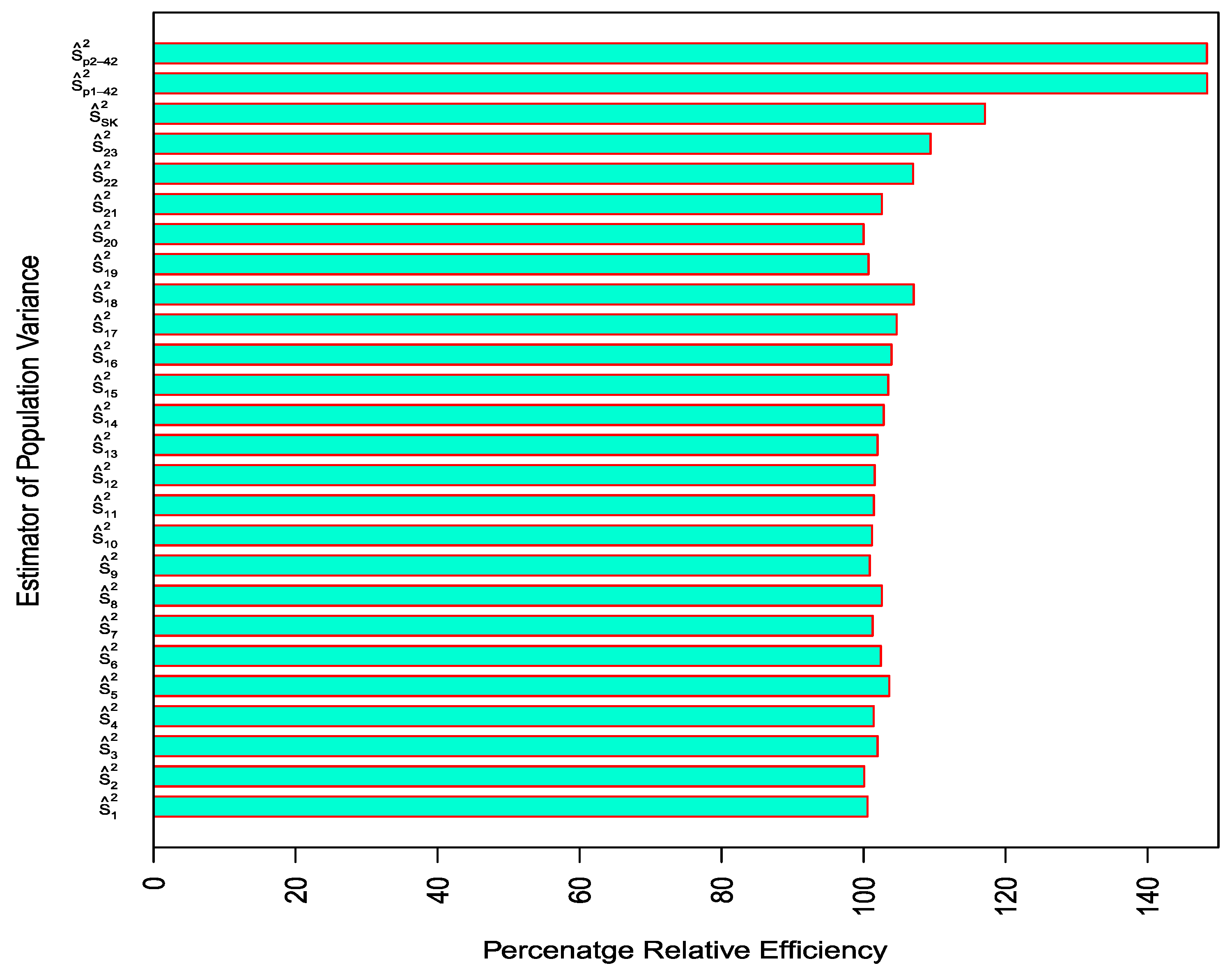
• The estimators proposed in class-I and class-II have higher PREs as compared to the existing estimators for both the populations considered in this study, which reveals the supremacy of the proposed classes of estimators in the presence of outliers in the data (cf. Table 5, Table 6, Table 7 and Table 8 and Figure 3 and Figure 4). For instance, the suggested estimators of class-I and class-II are at least 38% more efficient as compared to the traditional ratio estimator for population-I. For population-II, the efficiency of the suggested estimators exceeds 44%. All existing estimators are at most 11% and 17% more efficient as compared to the traditional ratio estimator for population-I and population-II, respectively.
• The class-I estimators have higher PREs as compared to class-II proposed in this study (cf. Table 7 and Table 8).
• The estimators which integrate information on the nonconventional dispersion parameter of the auxiliary variable and correlation coefficient between the study and auxiliary variables were found to be superior in terms of efficiency as compared to other estimators (cf. Table 7 and Table 8).
• The estimator which is based on inter-decile range and the correlation coefficient between the study and auxiliary variables turned out to be the most efficient estimator.
• It was also observed that the performance of existing estimators in comparison with the traditional ratio estimators is not much superior in the presence of outliers in the data (cf. Table 5 and Table 6), whereas the suggested estimators perform quite well as compared to the existing and the traditional ratio estimators (cf. Table 7 and Table 8). These findings highlight the significance of using nonconventional measures in estimating the population variance in the presence of outliers.

5. Conclusions

This study introduced two new classes of ratio- and regression-type estimators of population variance under simple random sampling without replacement by integrating information on nonconventional and somewhat robust dispersion measures of an auxiliary variable. The expressions for bias and mean square error were obtained, and the efficiency conditions under which the proposed estimators perform better than the existing estimators were also derived. In support of the theoretical findings, an empirical study was conducted based on two real populations which revealed that the suggested classes of estimators outperform the existing estimators considered in this study in terms of PREs in the presence of outliers. Based on the findings, it is strongly recommended that the proposed classes of estimators be used instead of the existing estimators to estimate the population variance in the case of outliers in the dataset. The present study can be further extended by estimating the population variance in the case of two auxiliary variables; moreover, under different sampling schemes, nonconventional measures can be employed to enhance the efficiency of the variance estimators.

References

1. Cochran, W.G. Sampling Techniques, 3rd ed.; John Wiley and Sons: New York, NY, USA, 1977. [Google Scholar]
2. Singh, H.P. Estimation of normal parent parameters with known coefficient of variation. Gujarat Stat. Rev. 1986, 13, 57–62. [Google Scholar]
3. Wolter, K.M. Introduction to Variance Estimation, 2nd ed.; Springer: New York, NY, USA, 1985. [Google Scholar]
4. Isaki, C.T. Variance estimation using auxiliary information. J. Am. Stat. Assoc. 1983, 78, 117–123. [Google Scholar] [CrossRef]
5. Kadilar, C.; Cingi, H. Ratio estimators for population variance in simple and stratified sampling. Appl. Math. Comput. 2006, 173, 1047–1058. [Google Scholar] [CrossRef]
6. Khan, M.; Shabbir, J. A ratio type estimator for the estimation of population variance using quartiles of an auxiliary variable. J. Stat. Appl. Probab. 2013, 2, 319–325. [Google Scholar] [CrossRef]
7. Maqbool, S.; Javaid, S. Variance estimation using linear combination of tri-mean and quartile average. Am. J. Biol. Environ. Stat. 2017, 3, 5–9. [Google Scholar] [CrossRef] [Green Version]
8. Muneer, S.; Khalil, A.; Shabbir, J.; Narjis, G. A new improved ratio-product type exponential estimator of finite population variance using auxiliary information. J. Stat. Comput. Simul. 2018, 88, 3179–3192. [Google Scholar] [CrossRef]
9. Naz, F.; Abid, M.; Nawaz, T.; Pang, T. Enhancing the efficiency of the ratio-type estimators of population variance with a blend of information on robust location measures. Sci. Iran. 2019. [Google Scholar] [CrossRef] [Green Version]
10. Solanki, R.S.; Singh, H.P.; Pal, S.K. Improved ratio-type estimators of finite population variance using quartiles. Hacet. J. Math. Stat. 2015, 44, 747–754. [Google Scholar] [CrossRef]
11. Subramani, J.; Kumarapandiyan, G. Variance estimation using median of the auxiliary variable. Int. J. Probab. Stat. 2012, 1, 36–40. [Google Scholar] [CrossRef] [Green Version]
12. Estimation of Variance Using Deciles of an Auxiliary Variable. Available online: https://www.researchgate.net/publication/274008488_7_Subramani_J_and_Kumarapandiyan_G_2012c_Estimation_of_variance_using_deciles_of_an_auxiliary_variable_Proceedings_of_International_Conference_on_Frontiers_of_Statistics_and_Its_Applications_Bonfring_ (accessed on 10 November 2019).
13. Subramani, J.; Kumarapandiyan, G. Variance estimation using quartiles and their functions of an auxiliary variable. Int. J. Stat. Appl. 2012, 2, 67–72. [Google Scholar] [CrossRef]
14. Upadhyaya, L.N.; Singh, H.P. An estimator for population variance that utilizes the kurtosis of an auxiliary variable in sample surveys. Vikram Math. J. 1999, 19, 14–17. [Google Scholar]
15. Yaqub, M.; Shabbir, J. An improved class of estimators for finite population variance. Hacet. J. Math. Stat. 2016, 45, 1641–1660. [Google Scholar] [CrossRef]
16. Subramani, J.; Kumarapandiyan, G. A class of modified ratio estimators for estimation of population variance. J. Appl. Math. Stat. Inform. 2015, 11, 91–114. [Google Scholar] [CrossRef] [Green Version]
17. Subramani, J.; Kumarapandiyan, G. Estimation of variance using known coefficient of variation and median of an auxiliary variable. J. Mod. Appl. Stat. Methods 2013, 12, 58–64. [Google Scholar] [CrossRef]
18. Upadhyaya, L.N.; Singh, H.P. Estimation of population standard deviation using auxiliary information. Am. J. Math. Manag. Sci. 2001, 21, 345–358. [Google Scholar] [CrossRef]
19. Riaz, M. A dispersion control chart. Commun. Stat.—Simul. Comput. 2008, 37, 1239–1261. [Google Scholar] [CrossRef]
20. Nazir, H.Z.; Riaz, M.; Does, R.J.M.M. Robust CUSUM control charting for process dispersion. Qual. Reliab. Eng. Int. 2015, 31, 369–379. [Google Scholar] [CrossRef]
21. Downton, F. Linear estimates with polynomial coefficients. Biometrika 1966, 53, 129–141. [Google Scholar] [CrossRef]
22. Gini, C. Variabilità e mutabilità. In Memorie di Metodologica Statistica; Pizetti, E., Salvemini, T., Eds.; Libreria Eredi Virgilio Veschi: Rome, Italy, 1912. [Google Scholar]
23. Hampel, F.R. The influence curve and its role in robust estimation. J. Am. Stat. Assoc. 1974, 69, 383–393. [Google Scholar] [CrossRef]
24. Shamos, M.I. Geometry and statistics: problems at the interface. In New Directions and Recent Results in Algorithms and Complexity; Traub, J.F., Ed.; Academic Press: New York, NY, USA, 1976; pp. 251–280. [Google Scholar]
25. Bickel, P.J.; Lehmann, E.L. Descriptive statistics for nonparametric models IV. spread. In Contributions to Statistics, Hajek Memorial Volume; Jureckova, J., Ed.; Academia: Prague, Czechia, 1979; pp. 33–40. [Google Scholar] [CrossRef] [Green Version]
26. Rousseeuw, P.J.; Croux, C. Alternatives to the median absolute deviation. J. Am. Stat. Assoc. 1993, 88, 1273–1283. [Google Scholar] [CrossRef]
27. Wu, C.; Zhao, Y.; Wang, Z. The median absolute deviations and their applications to Shewhart control charts. Commun. Stat.—Simul. Comput. 2002, 31, 425–442. [Google Scholar] [CrossRef]
28. Croux, C.; Rousseeuw, P.J. A class of high-breakdown scale estimators based on subranges. Commun. Stat.—Theory Methods 1992, 21, 1935–1951. [Google Scholar] [CrossRef]
29. Abid, M.; Abbas, N.; Nazir, H.Z.; Lin, Z. Enhancing the mean ratio estimators for estimating population mean using non-conventional location parameters. Rev. Colomb. Estadística 2016, 39, 63–79. [Google Scholar] [CrossRef]
30. Searls, D.T. Utilization of known coefficient of kurtosis in the estimation procedure of variance. J. Am. Stat. Assoc. 1964, 59, 1225–1226. [Google Scholar] [CrossRef]
31. Singh, D.; Chaudhary, F.S. Theory and Analysis of Sample Survey Designs; New Age International Publisher: New Dehli, India, 1986. [Google Scholar]
Figure 1. Boxplot of population-I.
Symmetry 12 00016 g001
Figure 2. Boxplot of population-II.
Symmetry 12 00016 g002
Figure 3. Comparison of PREs of existing and proposed estimators of variance for Population-I.
Symmetry 12 00016 g003
Figure 4. Comparison of PREs of existing and proposed estimators of variance for Population-II.
Symmetry 12 00016 g004