1. Introduction
Due to human over-exploitation, the global warming and energy crisis is a challenge that human beings must face. In order to achieve sustainable energy goals, developing renewable energy and improving energy efficiency are principal research methods. Power forecasting is important for power companies to improve energy efficiency. Power companies must closely monitor the supply and demand of electricity. Otherwise, whether the load demand is greater than the power supply capacity caused by a power jump, or the energy waste caused by an oversupply of electricity, the power cost for the power company will increase.
In recent years, the demand for electric power has been growing steadily along with booming economic growth in Taiwan. A stable electric power supply should be the basis for national economic development. A noticeable increase in demand for industrial and civil electricity has also been observed due to rapid economic development. A stable and sufficient electric power supply is most crucial to electric power companies. Electric power companies can reduce electric power operation costs and further improve the quality and stability of the electric power supply if the future load can be accurately forecasted.
Electric power load forecasting is of great importance. Therefore, electric power companies need to control the distribution of electric power. Excessive electric power supply will also cause grievous waste of energy, and on the other hand, a power trip will be caused if the load demand is greater than the electric power supply. In both cases, the electric power costs of electric power companies will be increased, such that civil electricity charges will be increased accordingly. The increase in civil electricity charges will lead to a rise in the costs of all things.
In view of the above reasons, it is necessary that effective electric power supply and maintenance of the appropriate reserve capacity and appropriate electric power distribution and dispatching are undertaken to determine the electric power demand increase due to various uncertainty factors. Moreover, reasonable electric power dispatching and distribution must be based on accurate load forecasting.
The quality of an electric power supply has a great influence on industrial development and living conditions. For the purpose of a stable electric power supply and eliminating heavy economic losses caused by power shortage, additional load increased by the demand for industrial development and civil electricity must be satisfied and an appropriate reserve capacity must be maintained. As a result, accurate load forecasting is extremely important.
Electric power load forecasting constitutes a part of an electric power system. Load forecasting can be classified into four categories according to time [
1]: Long-term, mid-term, short-term and ultra-short-term, as set out below, respectively:
Ultra-short-term load forecasting: The forecasting unit ranges from several minutes to several hours. Such a model is often used in flow control and used for detecting the stability of an electric power system and forecasting its reserve capacity, so as to prevent the occurrence of insufficient electric power dispatching.
Short-term load forecasting: The forecasting unit ranges from 1 h to several weeks. Such a model is often used for adjusting the economic dispatching of electric power, analyzing electric power demand and supply and power flow, forecasting crisis in the case of accidents, and for corporate operations and equipment maintenance.
Mid-term load forecasting: the forecasting unit ranges from several days to 1 month. Such a model is often used for estimating the peak electric power consumption and maintenance of power equipment. It can be used for detecting the time for maintenance and shutdown of power generators and is mainly used for decision making on energy management, such as electricity pricing and procurement of fuels used in power generation.
Long-term load forecasting: The forecasting unit ranges from 1 year to several years. Such a model is often used for research on electric power policies. New generator sets can be developed or constructed thereby for the future electric power planning of power industry, planning of power transmission and distribution system, procurement of fuels, signing contracts on outsourced electricity, electricity pricing and price structure analysis, corporate operation management and earnings estimation, load management, etc. This load forecasting considers the economic growth, energy proportion planning, industrial structure, construction of electric power development, electric power demand management and other conditions, such as population, temperature, power saving effect of research organizations or government agencies.
2. Literature Review
In [
2], Kuster et al. present a systematic review of electric power load forecasting. This paper reveals that regression methods are still popularity adopted and very efficient for long and very long-term electrical load forecasting. The machine-learning algorithms, such as artificial neural networks (ANN), support vector machines (SVM), and time series analysis are widely used for short and very short-term prediction.
Mi et al. [
3] propose a short-term power load forecasting method based on the improved exponential smoothing grey model. Authors used grey correlation analysis to determine the importance factor affecting the power load, then conducted power load forecasting using the improved multivariable grey model. The results showed that proposed method has a satisfactory prediction effect and meets the requirements of short-term power load forecasting.
Minhas et al. [
4] forecasted short-term electric power load based on the adaptive fuzzy neural system. In the ANN database, temperature and power load were used as a training model. The data of electric power load and temperature in 2015 were used for forecasting the electric power demand over the next few hours, and a fuzzy system was used for establishing membership functions. Subsequently, the probabilistic and stochastic hybrid adaptive fuzzy neural system was used for reducing the error in electric power load forecasting, in particular, the error on the weekend was much lower than that on weekdays.
Yin et al. [
5] proposed the ultra-short-term load forecasting method based on the weighted average optimal local shape similarity model which was used for acquiring the preliminary forecasting values of ultra-short term load and rectifying the preliminary forecasting values of the ultra-short term load. Computation methods for various influence factors were proposed after analyzing other factors influencing the accuracy of ultra-short-term load forecasting. Human comfort and other influence factors were improved based on the impact of the improved air quality index on human behaviors. The second rectification was carried out on the forecasting value of the ultra-short-term load by applying the Super-Stable Adaptive Control Theory, based on the deviation value of actual data from the forecasting data. Such a method features a very good adaptability to the computation speed and the accuracy of large-scale ultra-short term load forecasting and satisfies the actual demands of site engineering.
Din and Marnerides [
6] implemented applicability and comparison to the performance of the feed-forward deep neural network and recurrent deep neural network by leveraging the accuracy and computation capability of short-term forecasting. In that study, the data of 4 years were used for forecasting the load in several days or several weeks. The use of certain different input sources can accurately forecast the consumption of the short-term load. Such inputs included weather, time, official holidays and festivals. In addition, a higher accuracy can be obtained through feature analysis of the time frequency of collaborative use of the deep neural network.
Chen et al. [
7] proposed a kind of nonlinear issue of partially connected neural network to be used for short-term load forecasting and have developed the group-based chaos genetic algorithm to produce various effective neural networks. In that study, a new pruning method was utilized to develop partially connected neural networks. In order to further improve forecasting accuracy, a non-linear partially connected neural network predictor based on the neural network has been developed in the paper. As a result of the application of this research, results in a PJM market dataset and an ISO New England dataset with errors of 1.76% and 1.29% have been obtained, respectively, which has proven that the network is an effective predictor.
Eljazzar et al. [
8] introduced the main factors to short-term load forecasting, such as temperature, wind and humidity. They studied the relationship between inputs and peak load and measured the accuracy through comparison between actual value and forecasting value, residual error and the fitted model. Selection of correct parameters affecting forecasting was very important. Additional computation time would be required, and forecasting accuracy may not be improved if irrelevant parameters were selected. They introduced the impact of electric power load factors on short-term load forecasting, and applied certain factors (temperature, required temperature, wind and humidity) in ANN, so as to understand their impact on electric power load forecasting in the north of Cairo. The experimental results showed that MAPE, RMSE and MAE were reduced by more than a half as a result of the application of the model proposed.
López et al. [
9] proposed the application of a linear hybrid model in short-term load forecasting. That study was in relation to load forecasting of a current Spanish Transport System Operator based on linear autoregressive techniques and neural networks. At present, the forecasting system forecasts load in each area in Spain respectively, to enable the load behaviors in each area to be subject to the effects of the same factors. Subsequently, certain areas have been integrated as a linear hybrid model, so as to utilize the information from other areas to understand the general behaviors of all areas, as well as to determine the individual deviation of each area. Such a technique is particularly useful for the modeling of impact of special days without sufficient information. Such a model has been applied in the three most relevant areas in the system, to collect the data of several years for the training of the model and forecast the demand load for the whole year. The proposed model provided a powerful database and average error was reduced by 4% through comparison between the experimental result and the original autoregressive model.
Tian et al. [
10] proposed a hybrid deep learning model that integrates the hidden feature of the convolutional neural network (CNN) model and the long short-term memory (LSTM) model to improve the forecasting accuracy. The CNN extracts the local trend and captures the same pattern, and the LSTM learns the relationship in time steps. The performances of the hybrid model proposed by this paper were compared with the LSTM model and the CNN model; the experimental results showed that the proposed method can achieve a better and a more stable performance than either the CNN, or LSTM modes.
Semero et al. [
11] proposed a hybrid technique for very short-term load forecasting in microgrids. The proposed method integrated genetic algorithm (GA), particle swarm optimization (PSO), and adaptive neuro fuzzy inference systems (ANFIS). The GA selects important predictors that significantly influence the load pattern among a number of candidate input variables. The PSO is used to optimize an ANFIS model for very short-term forecasting of load.
3. Proposed Method
In this study, preliminary forecasting values of electric power load were executed by integrating ANFIS and BPN and persistence. The preliminary forecasting values of the electric power load obtained therefrom were called suboptimal solutions and finally the optimal weighted value was determined by applying the search algorithm through integrating the above three methods into a forecast formula by weighting, in order to effectively improve forecasting accuracy.
3.1. Adaptive-Network-Based Fuzzy Inference System (ANFIS)
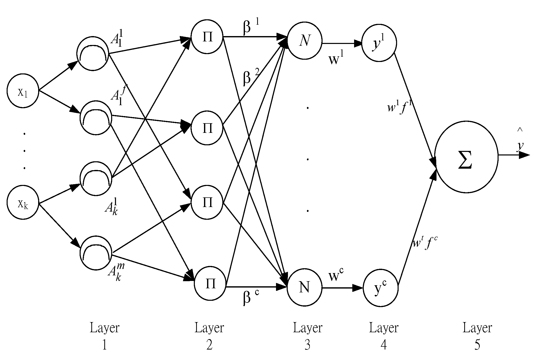
In this study, the IF-THEN rules of fuzzy system were developed systematically through input and output data by applying an artificial neural algorithm to adjust the parameters of ANFIS with the Sugeno model, as shown in
Figure 1. In this paper, the architecture of ANFIS was utilized to forecast the electric power load value. A common IF-THEN rule of the Sugeno model is the flowing:
In this study, the ANFIS was applied with three input nodes and an output node. Let X= (x1, x2, x3,) be input load data; from x1 to x3 in sequence, x1 was the load value for the first period of time prior to the forecasting time point, x2 was the load value for the second period of time; x3 was the load value for the third period of time. The node at the output layer was the forecasting value of electric power load at the forecasting time point.
ANFIS was a five-layer artificial neural node. Set out below are the functions of each layer [
12]:
Layer 1: In the architecture of ANFIS as shown in
Figure 1, each node at the layer 1 was represented with
i to indicate the membership function of antecedent input variables. Node function output was as shown in Equation (1), indicating the membership grade of output to its corresponding fuzzy set. The membership function could be any appropriate function, such as the Bell Function or Gaussian Function.
where
is the
j-th input,
is the output of Layer 1 and the
is the membership grade of a fuzzy set
.
Layer 2: Each node at the layer was marked with
i to indicate that each node implemented arithmetic product computation to incoming signal. The node output was as shown in Equation (2), indicating the output of each rule.
where
is the membership grade of the input
xj that is fed to node
i of Layer 2. The output of each node of layer 2 represents the firing strength of a rule.
Layer 3: Each node at the layer was marked with
i to calculate the ratio of the output of the
ith rule to the sum of outputs of all rules. It was called normalized fulfillment, as shown in Equation (3).
where
c is the number of rules.
Layer 4: Each adaptive node, marked with
i, at the layer represented an output variable of consequent explicit function and was used for completing the computation as shown in Equation (4); where,
c was the number of rules.
where
is the output of layer 3 and
is the parameter of rule.
Layer 5: Only a single node at the layer was used for calculating the sum of outputs of all rules, as shown in Equation (5).
3.2. Ultra-Short Term Load Forecasting Based on Back-Propagation Neural Network
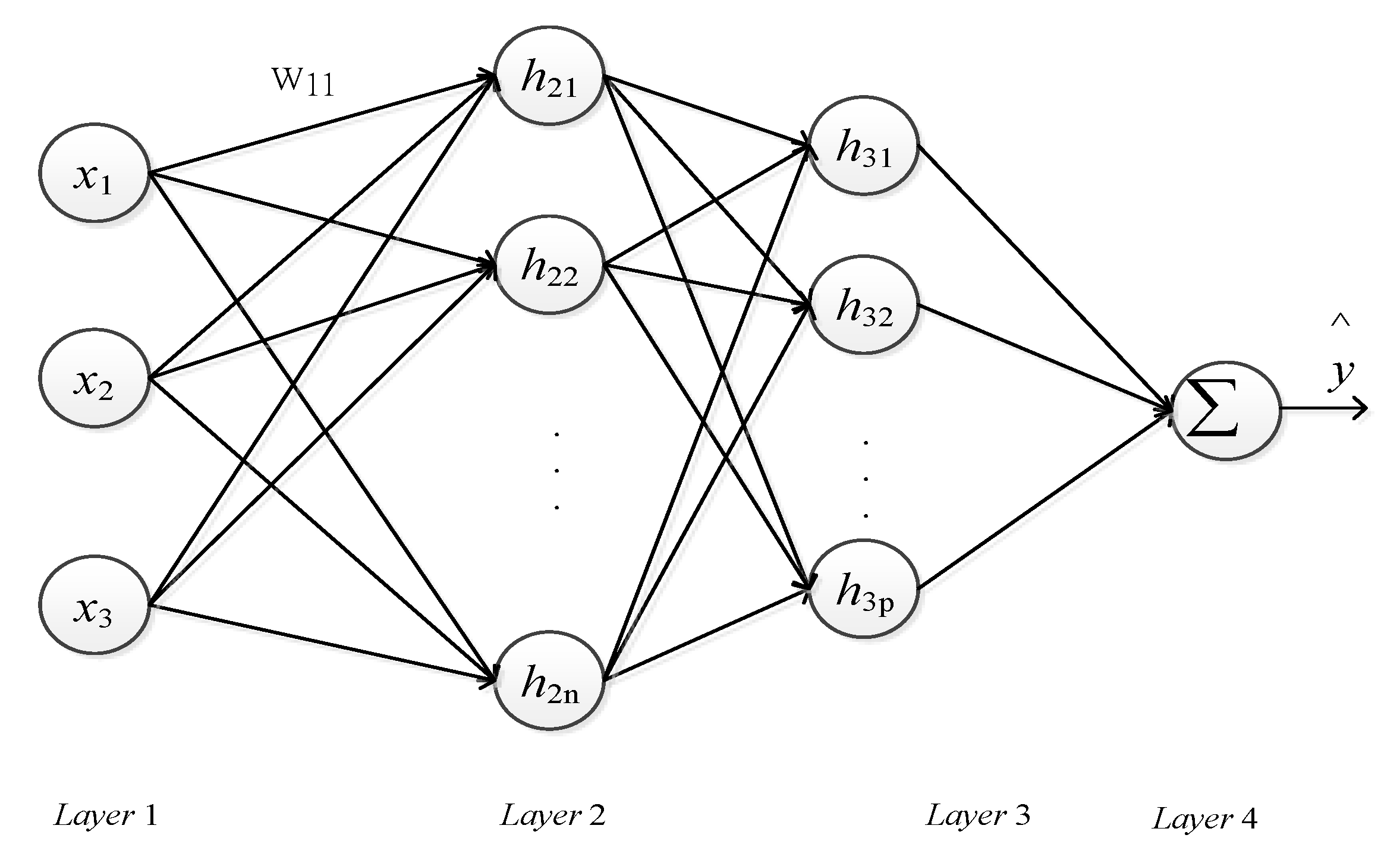
Operation of the BPN consisted of two parts: learning and recalling. Supervised learning was used in the learning part. Supervised learning acquired training data and target output value from the problem and imported training value into the system, and repeatedly adjusted the weighted value and bias through the Steepest slope method. In terms of the recalling part, through classification and forecasting, the network would inform us of the most possible forecasting result when a value has been imported. The BPN was applied to forecast electric power load value in this paper, as shown in
Figure 2.
In this paper, the architecture of the BPN for electric power load forecasting used three input nodes and one output node. Nodes x1 to x3 at the input layer were the actual values of electric power load for the three periods of time prior to forecasting. The gradient descent approach is adopted for adjusting the parameters of the BPN. The node at the output layer was the forecasting value of the electric power load in the forecasting period of time.
3.3. Persistence
In terms of persistence, it was assumed that the future load was as the same as the load during forecasting [
13]. In short-term load forecasting, persistence showed a higher accuracy than other load forecasting methods. The forecasting accuracy of persistence, however, reduced along with the increase of forecasting time [
14].
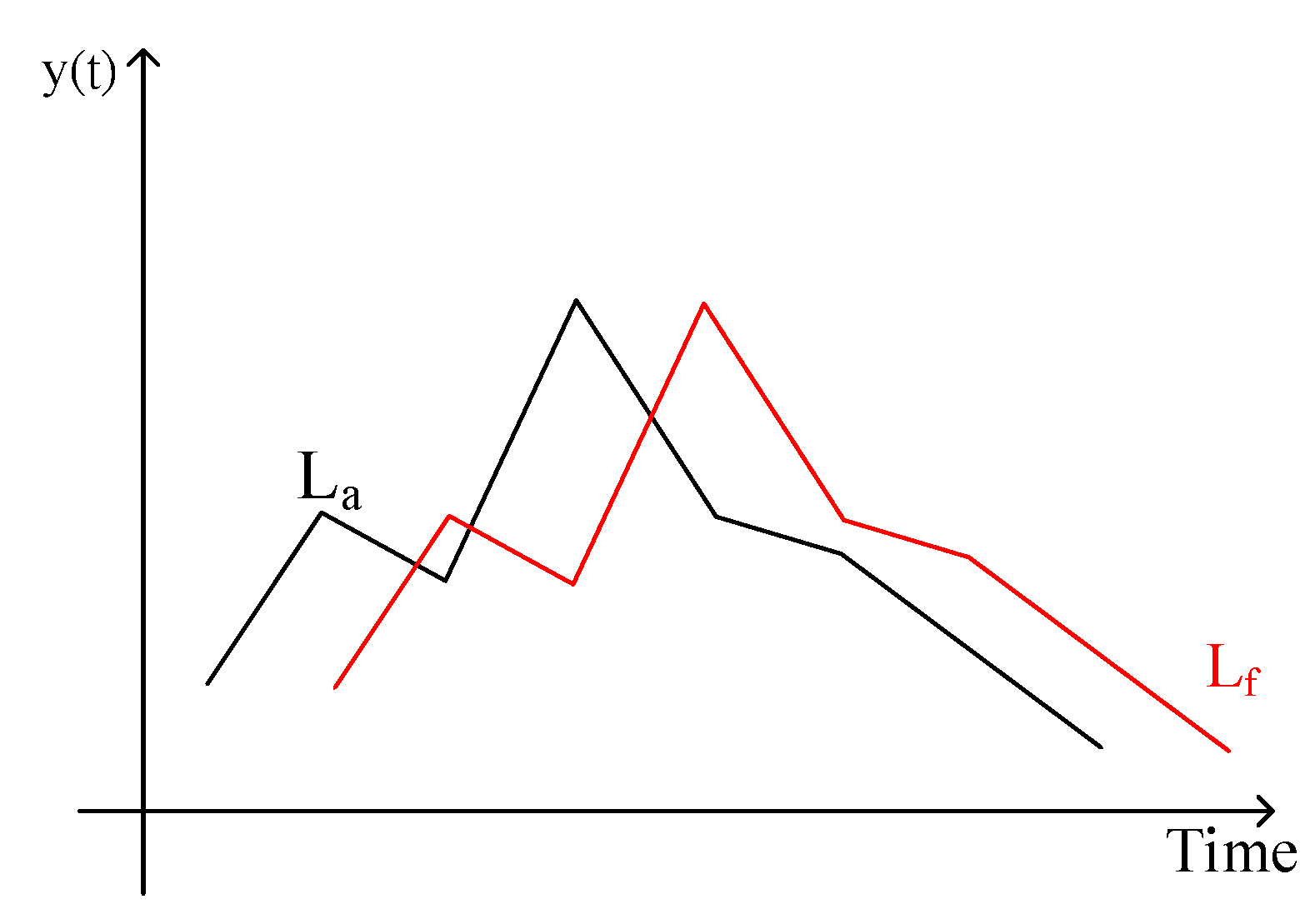
Figure 3 is the curve graph of persistence.
La is the current actual load value;
Lf is forecasting value. As seen, the value of
Lf was forecasted from the first period of time on the first day prior to the actual load value to the next period of time in sequence. However, in the case of bad weather or hot weather, such external conditions would lead to dramatic changes in the load line and hence forecasting based on persistence would not be so accurate. If the weather conditions and other external factors on that day are the same as that on the previous day, the forecasting based on the method will be quite accurate. Persistence is one of the most efficient methods in some cases.
Persistence was a method for forecasting the reference value and was applicable when there was a stable environment during electric power load forecasting, without any factor which would cause dramatic changes of load. In this case, persistence would be significantly useful. In the application of persistence in electric power load forecasting, a set of data of actual load values per 10 min in the previous period of time was regarded as the forecasting value of electric power load in the next period of time. Such a method is the traditional method for forecasting the reference value, as shown in Equation (6):
where,
Lf (
t + 1) is the forecasting value of time
t+1,
La is the actual value of time
t.
3.4. Integrated Search Method
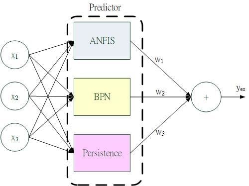
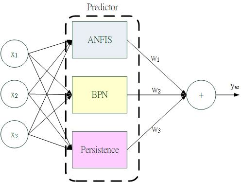
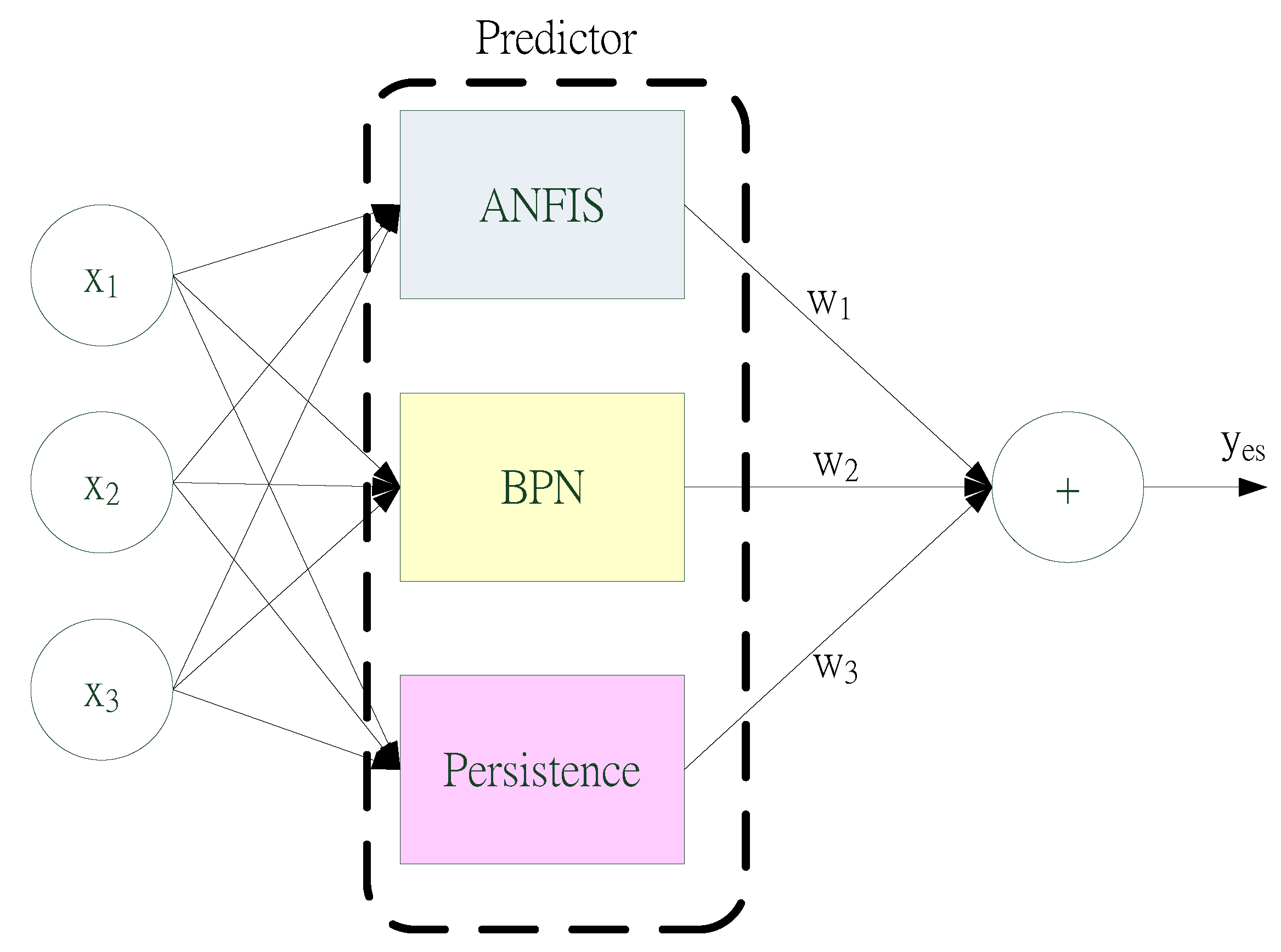
Figure 4 shows the diagram of the proposed predictor for an ultra-short-term power load forecasting. In
Figure 4, this paper integrated three methods, ANFIS, BPN and persistence, into the predictor. Each method was a suboptimal solution, attached with a weight (0
wi 1,
i = 1,2,3);
w1 +
w2 +
w3 = 1; and the output
yes was evaluated as Equation (7).
where
y1,
y2;
y3 are the outputs of ANFIS; BPN; and persistence, respectively. The optimal weight value was determined by applying the search algorithm, as shown in Algorithm 1.
In order to determine the best weighted value, Equation (8) was regarded as the criterion for evaluating weight in this paper.
where, the restriction was 0
wi 1,
i = 1,2,3, and
w1+
w2+
w3 = 1.
was actual load value;
n was data volume. In Equation (8), all training data were used for calculating the difference between the weight of load estimates of the three methods and the actual load value, and obtaining the
wi at the time of the minimal error value as the weight of training model.
| Algorithm 1. Integrated search algorithm |
| Input: ANFIS, BPN, Persistence model, load dataset (X, ) |
| Output: w1,opt, w2,opt, w3,opt |
| Step | 1: | Input X, calculate ANFIS, BPN, Persistence output: y1, y2, y3. |
| Step | 2: | Emin = |
| Step | 3: | For w1 = 0: 1: step 0.01 |
| Step | 4: | For w2 = 0: (1 − w1): step 0.01 |
| Step | 5: | w3 = 1 − (w1+w2) |
| Step | 6: | |
| Step | 7: | If (Emin > ) Then |
| Step | 8 | Emin = ; w1,opt = w1;w2,opt = w2; w3,opt = w3; |
| Step | 9 | End if |
| Step | 10 | Next w2 |
| Step | 11 | Next w1 |
| Step | 12 | End |
4. Experimental Results
4.1. The Data Set
In this paper, electric power consumption in workdays and non-workdays in Taiwan was forecasted. Generally, work and rest hours in weekdays are roughly the same, therefore, the electric power load is stable. In holidays, the rest of certain industries causes a load different from that in weekdays. Therefore, forecasting was carried out in respect of two periods of time respectively, i.e., workdays and non-workdays, in this paper. Sample data derived from the daily electric power supply of the Taiwan Power Company. A set of data was acquired per 10 min, and a total of 144 sets of data were collected each day. In this paper, a total of seven modes were established on a weekly basis, and the simulation was implemented in one model on each day of each week. In the phase of model training, data on the same day in three consecutive weeks were used for training. For example, sample data on 31 May 2017, 7 June 2017 and 14 June 2017 were used as model training data. Upon the completion of model training, the model was used for forecasting the electric power consumption on the same day in the next week, i.e., 21 June 2017. There were three inputs for each model training, i.e., x
1, x
2, x
3. x
1 was the load value for the first period of time prior to the forecasting time point; x
2 was the load value for the second period of time, and x
3 was the load value for the third period of time. Output y
i(
t),
i = 1, 2, 3 was the load at the forecasting time point,
t;
was the actual load. In model training, define
as the error value. For adjustment of parameters, please refer to [
15].
Four methods were used in this study for ultra-short-term electric power load forecasting. The first method was ANFIS, the second method was BPN, the third method was persistence, and the fourth method was integrated search. In respect of all the four methods, actual values of electric power load were used as test data and error values were used to compare and judge the forecasting accuracy of the four methods.
4.2. Ultra-Short Term Electric Power Load Forecasting
In this paper, ANFIS used three input nodes and one output node. Inputs were the electric power load values for the first three periods of time prior to forecasting. Generally, load forecasting started from 00:00 each day to 23:55 next day. Data from Taiwan Power per 10 min were used as a set of training data. Therefore, data of the three periods of time prior to forecasting, i.e., the actual load values in the first period of time as at 11:50, the second period of time as at 11:40 and the third period of time as at 11:30, were used as training data.
Three input nodes and one output node were used in the architecture of BPN. The output layer was the forecasting value of electric power load during forecasting period of time.
In terms of persistence, a set of data of actual load values per 10 min in the previous period of time were used as the forecasting value of electric power load during forecasting period of time.
The integrated search has integrated the above three methods, i.e., BPN, ANFIS and persistence. Preliminary forecasting values of electric power load from the above three methods were called suboptimal solutions and the optimal weighted value was determined through search by integrating the three forecasting methods.
In order to express the error of each method, Mean Absolute Percentage Error (MAPE) and Maximum Absolute Percentage Error (MaxAPE) were used in this paper to calculate and compare error values, as shown below:
(1) Mean Absolute Percentage Error (MAPE,
Eave):
where:
PL was the actual load value at the time
t,
Pf was the forecasting load value at the time
t.
(2) Maximum Absolute Percentage Error (MaxAPE,
Emax):
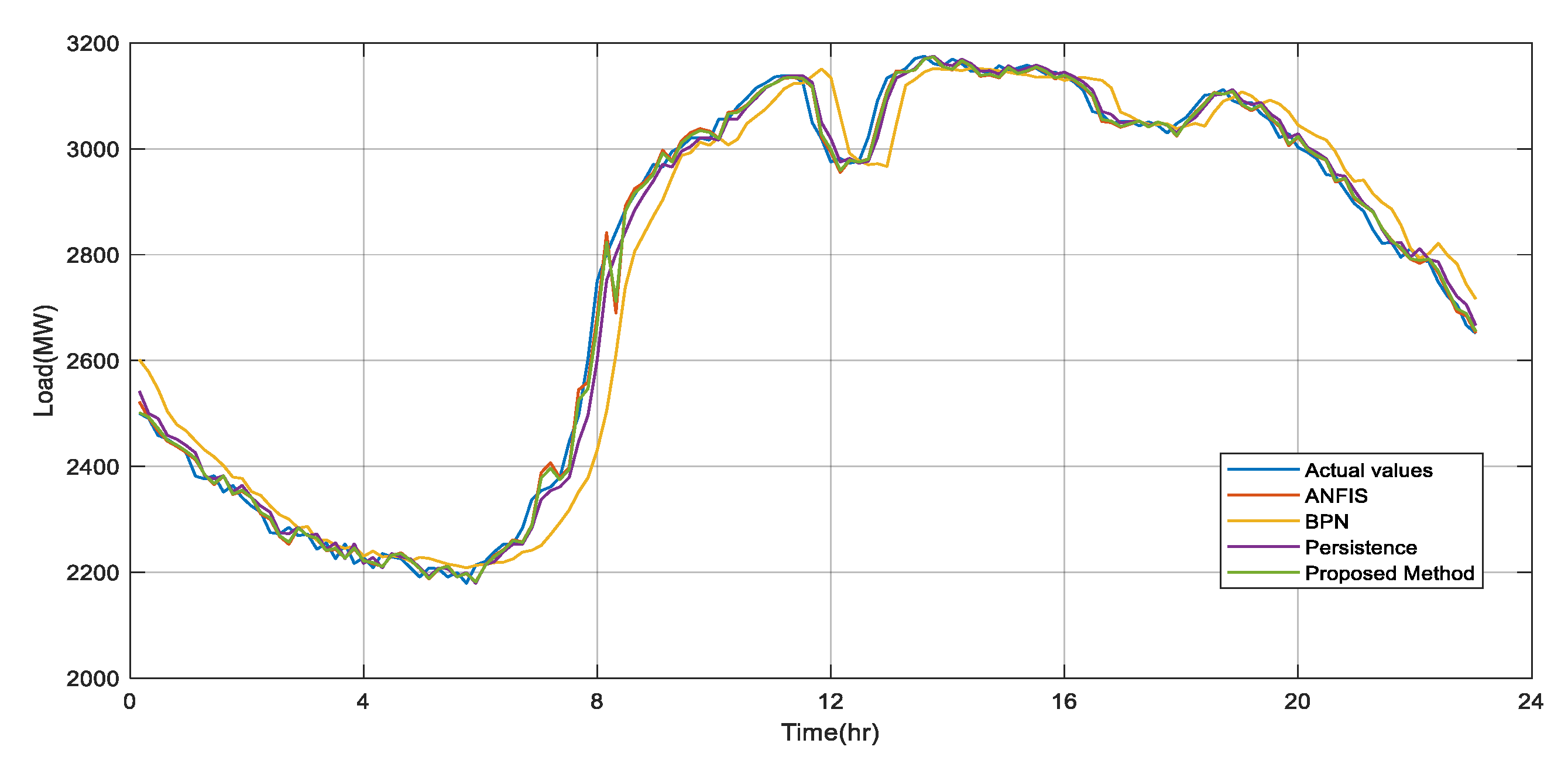
4.2.1. Workday Ultra-Short-Term Electric Power Load Forecasting Experiment
In the experiment, forecasting object was the ultra-short-term electric power load in northern Taiwan on Wednesday, 21 June 2017. Comparison between the forecasting values of ultra-short-term electric power load by applying ANFIS, BPN, persistence, and integrated search and the actual load values are as shown in
Figure 5. In
Figure 5, the blue line represents the actual values; the red line represents the forecasting values of ANFIS; the yellow line represents the forecasting values of BPN, the purple line represents the forecasting values of persistence, and the green line represents the forecasting values of the integrated search.
Table 1 sets out the comparison of errors in forecasting workday electric power load in northern Taiwan from 20 June to 26 June.
Table 2 sets out the comparison of MAPE and MaxAPE in five workdays. As seen, the average error of the solution proposed in the five days, no matter absolute error or maximum error, is lower than that of ANFIS, BPN and persistence.
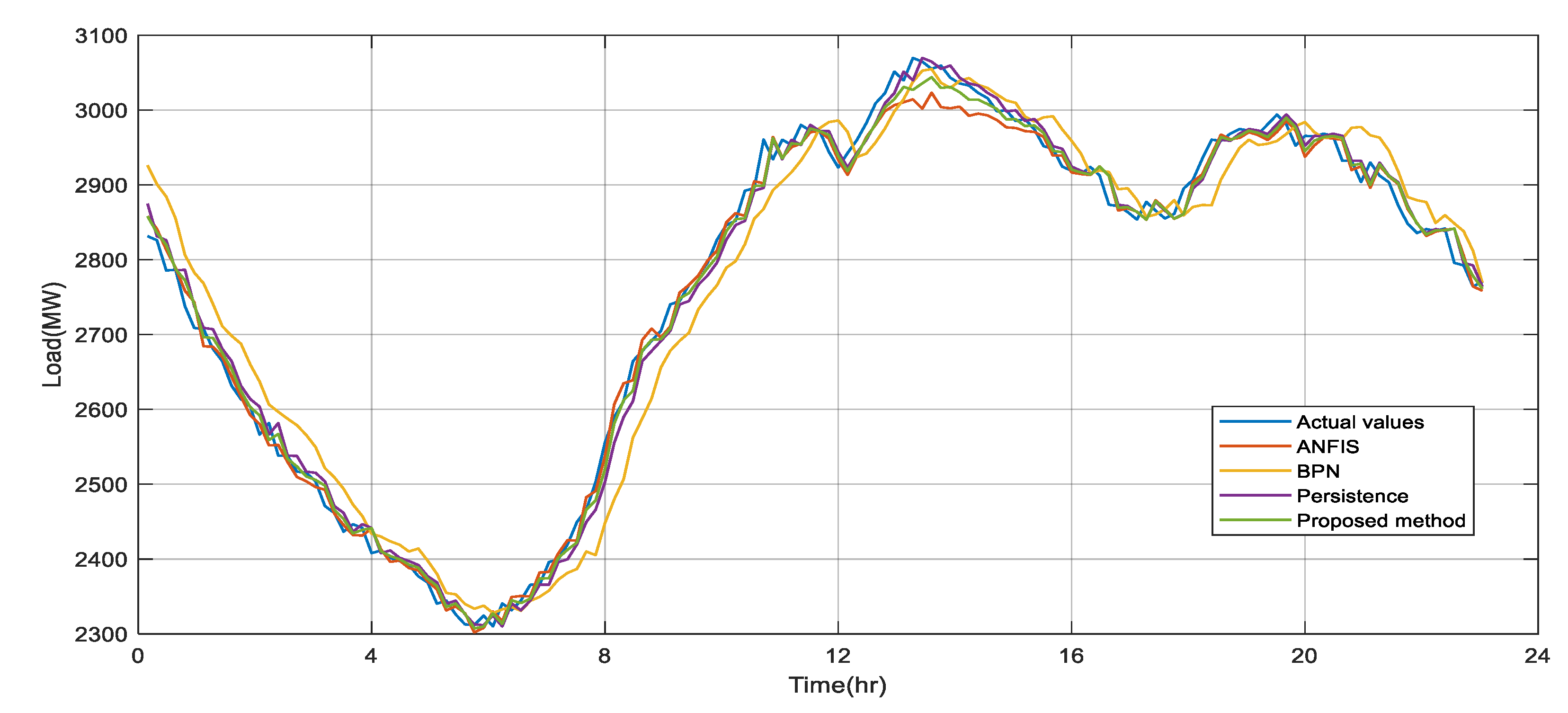
4.2.2. Non-workday Ultra-Short-Term Electric Power Load Forecasting Experiment
Figure 6 shows the comparison of load forecasting in northern Taiwan on a non-workday, i.e., Saturday, 24 June 2017.
In
Figure 6, the blue line represents the actual values; the red line represents the forecasting values of ANFIS; the yellow line represents the forecasting values of BPN, the purple line represents the forecasting values of persistence, and the green line represents the forecasting values of integrated search.
Table 3 sets out the comparison of load forecasting errors in non-workdays in northern Taiwan on 24 June and 24 June.
Table 4 shows the comparison of MAPE and MaxAPE in non-workdays. As seen, the average error of the solution proposed in non-workdays, no matter absolute error or maximum error, is lower than that of ANFIS, BPN and persistence.
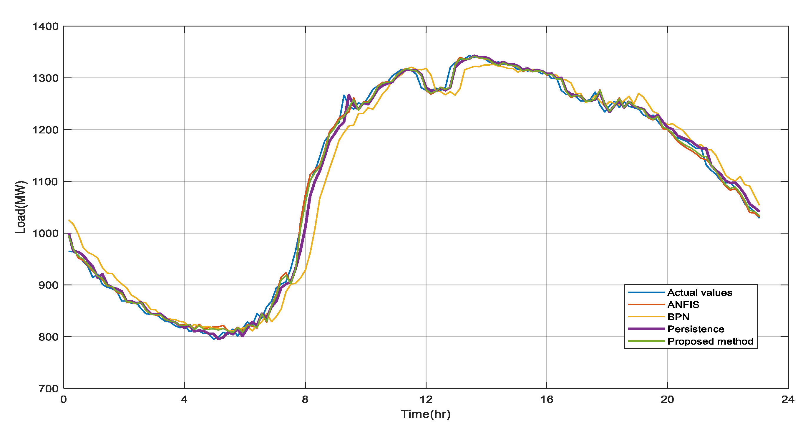
4.2.3. National Workday Ultra-Short-Term Electric Power Load Forecasting Experiment
In order to forecast workday ultra-short-term electric power load across Taiwan, ANFIS, BPN and persistence, and integrated search were used in this paper to forecast electric power consumption load across Taiwan on 20 June 2017. Comparison results are as shown in
Figure 7. The representation of lines in
Figure 7 is the same as that in above experiments.
Table 5 sets out the comparison between the solution proposed and the other three methods in workdays across Taiwan.
Table 6 sets out average errors. As seen, the average error of the solution proposed is lower than that of the other three methods.
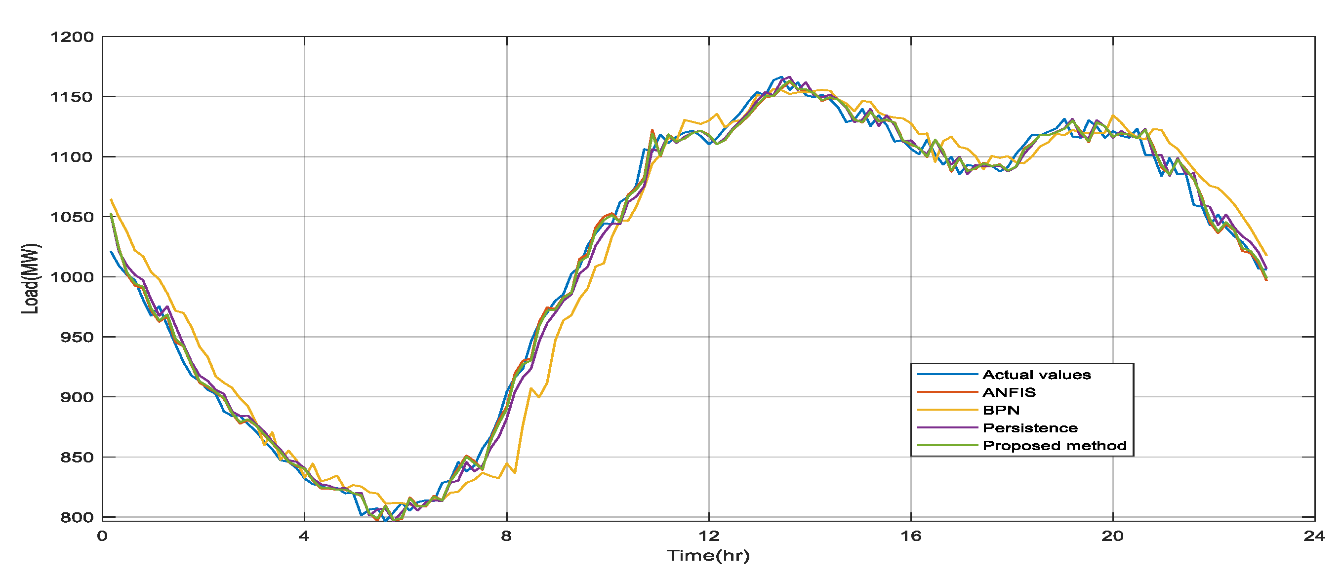
4.2.4. National Non-Workday Ultra-Short-Term Electric Power Load Forecasting Experiment
Non-workday electric power load across Taiwan was also forecasted in this paper.
Figure 8 shows the comparison of ultra-short-term electric power load forecasting on 24 June 2017 between the solution proposed in this paper and the other three methods. The representation of lines in
Figure 7 is the same as that in above experiments.
Table 7 sets out forecasting errors in non-workdays across Taiwan in June.
Table 8 sets out average errors in non-workdays across Taiwan. As seen, the average error of the solution proposed is lower than that of the other three methods.
5. Discussion
An integrated electric power load forecasting method was proposed in this paper. ANFIS, BPN and persistence were integrated by weighting, and the optimal weighted value was determined by applying the search algorithm. The MAPE and MaxAPE analysis of experimental results indicated that among the three methods of ANFIS, BPN and persistence, ANFIS features a better forecasting accuracy. But the result through the weighted integrated search proposed in this paper showed that the solution proposed in this paper showed a better forecasting accuracy than ANFIS. The optimal weighted value can be determined by applying integrated search. In addition, significant effect will be observed if integrating more efficient forecasting methods in the future. It can be effectively applied by practitioners in certain relevant fields.
In this paper, actual load data in the three periods of time prior to forecasting were used to forecast electric power load. Such a practice is relatively not subject to the great influence of weather or other factors. In the future, data in relation to load, such as temperature, weather, apparent temperature, relative humidity, wind force and daylight hours can be utilized to increase the accuracy of the system in forecasting. In this paper, the search algorithm was employed to determine the optimal weighted value. In future study, the genetic algorithm, bee colony algorithm and other optimization theories can be used to determine the optimal weighted portfolio, so as to achieve better forecasting performance.
The search algorithm determines the w1, w2, and w3 parameter values. Since there are only three parameters to decide, using the search algorithm can find the best value in a short time. Since the current load value is estimated using the power load values of the previous three 10-min periods, the experimental results show that the predicted value of this paper is more accurate than the other three methods. When future research considers long-term or mid-term electric power load forecasting, the search algorithm requires more calculation time because of the longer estimation time and the need to consider the weather and temperature. In future research, gene algorithms, bee colony algorithms, and PSO algorithms can be used to estimate parameters for long-term or mid-term electric power load forecasting.


