Locality Sensitive Discriminative Unsupervised Dimensionality Reduction

Abstract

Graph-based embedding methods receive much attention due to the use of graph and manifold information. However, conventional graph-based embedding methods may not always be effective if the data have high dimensions and have complex distributions. First, the similarity matrix only considers local distance measurement in the original space, which cannot reflect a wide variety of data structures. Second, separation of graph construction and dimensionality reduction leads to the similarity matrix not being fully relied on because the original data usually contain lots of noise samples and features. In this paper, we address these problems by constructing two adjacency graphs to stand for the original structure featuring similarity and diversity of the data, and then impose a rank constraint on the corresponding Laplacian matrix to build a novel adaptive graph learning method, namely locality sensitive discriminative unsupervised dimensionality reduction (LSDUDR). As a result, the learned graph shows a clear block diagonal structure so that the clustering structure of data can be preserved. Experimental results on synthetic datasets and real-world benchmark data sets demonstrate the effectiveness of our approach.

1. Introduction

Due to the large number of data generated by the advancements of science and technology, dimensionality reduction has become an important task in data mining and machine learning research with many applications [1,2,3,4]. These data have such characteristics as high dimensionality, nonlinearity, and extreme complexity, which bring a lot of problems to the subsequent data processing. However, the intrinsic structure of data are often suspected to be much lower due to the redundant information hidden in the original space [5]. Therefore, revealing the potential low-dimensional representation involved in the corresponding high-dimensional structure is an essential preprocessing step for various applications. Under the background, a lot of supervised and unsupervised dimensionality reduction methods are proposed, such as principal component analysis (PCA) [6], linear discriminant analysis (LDA) [7], Laplacian embedding(LE) [8,9,10], local linear embedding (LLE) [11], locality preserving projections (LPP) [12], neighborhood minmax projections (NMMP) [13], isometric feature mapping (IsoMAP) [14], discriminant sparsity neighborhood preserving embedding (DSNPE) [15], and multiple empirical kernel learning with locality preserving constraint (MEKL-LPC) [16], etc. Obviously, the unsupervised dimensionality reduction method is more challenging than other methods due to the lack of label information. Among them, the graph embedding method exhibits significant performance because it captures the structural information of high-dimensional space. The graph embedding method is built on the basis of manifold assumption, which means the data are formed according to a certain manifold structure and the nearby data points tend to have the same labels.

The commonly used graph-based algorithms, such as LPP [12], IsoMAP [14], local graph based correlation clustering (LGBACC) [17], and locality weighted sparse representation (LWSR) [18] generally have the same steps—for instance, (1) build adjacency graph for each neighborhood; (2) construct pairwise feature (similarity) for each neighborhood to describe the intrinsic manifold structure; and (3) convert the problem into an eigenvalue problem. Thus, we can find the traditional graph-based algorithms mentioned above are all established independently of the subsequent processes, i.e., cluster indicators need to be extracted through post-processing, such dimensionality reduction results are highly dependent on the input pairwise feature matrix [19]. For graph-based algorithms taken, only local distances’ account in the original space cannot adequately eliminate noise and capture the underlying manifold structure [20], in that it is an insufficient description for data similarity. Moreover, it is usually difficult to explicitly capture the intrinsic structure of data only by using pairwise data during the graph construction process [21]. In fact, for pairwise data, the similarity is dependent on the adjacency graph constructed by a pair of data individually, without consideration for the local environment of pairwise data. It can be seen from Figure 1, though the distance between A and B is shorter than that between A and C in the original space, and, clearly, $S(A,B)$ is called a similarity, one pairwise feature is bigger than $S(A,C)$, hence point A and point C should be sorted out to one class, and B to the other class. However, point A and point C could get more similar in regular classification or clustering tasks because there exists a dense distribution of many points which link A and C, resulting from a big gap between A and B, which are regarded as less similar in some traditional methods with two more manifold and consequently divided into different class. Therefore, the traditional definition of similarity does not sufficiently describe the structure.

In recent years, there has been a lot of research devoted to solving these problems. For example, the constrained Laplacian rank (CLR) method [22] learns a block diagonal similarity matrix so that the clustering indicators can be immediately extracted. For Cauchy graph embedding [23], a new objective is proposed to preserve the similarity between the original data for the embedded space, and emphasize the closer two nodes in the embedding space, those that are more similar. Projected clustering with adaptive neighbors (PCAN) [24] designs a similarity matrix and is assigned adaptive and optimal neighbors to every piece of data on the basis of the local distances to learn instead of learning a probabilistic affinity matrix before dimensionality reduction. Stable semi-supervised discriminant learning (SSDL) [25] is worked out to learn the intrinsic structure of a constructed adjacency graphs which could extract the local topology characteristics, and get the geometrical properties as well. Nonetheless, these methods only focus on parts of the problems mentioned above, and the challenge in reasonably representing underlying data structure or adaptively adjusting the similarity graph still exists. As a consequence, it is quite necessary and challenging to develop an algorithm to address these problems.

In this paper, we propose a novel adaptive graph learning method, namely locality sensitive discriminative unsupervised dimensionality reduction (LSDUDR), which aims to uncover the intrinsic topology structures of data by proposing two objective functions. In the first step, one of the objective functions is aimed at guaranteeing the mapping of all points close to each other in the subspace, while the other one is with the purpose of excluding points with a large distance from the subspace. Furthermore, a data similarity matrix is learned to adaptively adjust the initial input data graph according to the basis of the projected local distances, that is to say, we adjust the projection jointly with graph learning. Moreover, we constrain the similarity matrix by imposing a rank constraint to make it contain more explicit data structure information. It is worthwhile to emphasize the main contributions of our method: (1) LSDUDR can construct a discriminative linear embedded representation that can deal with high-dimensional data and characterize the intrinsic geometrical structure among data; (2) compared with traditional two-stage graph embedding methods, which need an independent affinity graph to be constructed in advance in LSDUDR, and a clustering-oriented graph can be learned and the clustering indicators are extracted with no post-processing needed for the graph; (3) comprehensive experiments were performed on both synthetic data sets and real world benchmark data sets and better effectiveness of the proposed LSDUDR was demonstrated.

2. Related Work

2.1. Principal Component Analysis (PCA)

PCA is one of the most representative unsupervised dimensionality reduction methods. The main idea of PCA is to seek a projection transformation to maximise the variance of data. Assume that we have a data matrix $X\in R^{d\times n}$, where $x_i\in R^{d\times 1}$ denotes the i-th sample. For better generality, the samples in the data set are centralized, i.e., ${\displaystyle {\displaystyle \sum _{i=1}^n}}{x}_i=0$. PCA aims to solve the following problem:

$$\begin{array}{c}{\displaystyle \underset{W^{T}W=I}{max}}{\displaystyle \sum _{i,j=1}^n}{∥W^T{x}_i-W^T{x}_j∥}_2^2,\hfill \end{array}$$

(1)

where $W\in R^{d\times m}$ is the projection matrix, and m is the dimensionality of the linear subspace. When data points lie in a low-dimensional manifold and the manifold is linear or nearly-linear, the low-dimensional structure of data can be effectively captured by a linear subspace spanned by the principal PCA directions; the property provides a basis for utilizing the global scatter of samples as regularization in many applications.

2.2. Locality Preserving Projections (LPP)

LPP is very popular to substitute algorithms in linear manifold learning in which the data are projected responding to the direction of maximal variance, and the adjacent graph was employed to extract the structure properties of high-dimensional data, and structure properties were transplanted into low-dimensional subspace. The objective function of LPP is

$$\begin{array}{c}{\displaystyle \underset{W^{T}W=I}{min}}{\displaystyle \sum _{i,j=1}^n}{∥W^T{x}_i-W^T{x}_j∥}_2^2{s}_{ij},\hfill \end{array}$$

(2)

where $s_{ij}$ is defined as the similarity between samples $x_i$ and $x_j$. As we can see, LPP is a linear version of Laplacian Eigenmaps that uses linear model approximation to nonlinear dimensionality reduction, Thus, it shares many of the data representation properties of nonlinear techniques such as Laplacian eigenmaps or locally linear embedding.

2.3. Clustering and Projected Clustering with Adaptive Neighbors (PCAN)

The PCAN algorithm performs subspace learning and clustering simultaneously instead of learning an initial pairwise feature matrix that is constructed before dimensionality reduction. The goal of PCAN is to assign the optimal and adaptive neighbors for each data point according to the local distances so that it can learn a new data similarity matrix. Therefore, it can be used as a clustering method, and can also be used as a unsupervised dimensionality reduction method. Denote the total scatter matrix by $S_t=XH{X}^T$, where H is the centering matrix defined as $H=I-\frac{1}{n}\mathbf{1}{\mathbf{1}}^T$, and $\mathbf{1}$ is a column vector whose elements are all 1. PCAN constrains the subspace with $W^T{S}_{t}W=I$ so that the data in the subspace has no statistical correlation. In [24], the definition of PCAN is:

$$\begin{array}{c}{\displaystyle \underset{S,W}{min}}{\displaystyle \sum _{i,j=1}^n}\left({∥W^T{x}_i-W^T{x}_j∥}_2^2{s}_{ij}+\theta s_{ij}^2\right)\hfill \\ s.t.\forall i,{\mathbf{s}}_i^T\mathbf{1}=1,0\le s_{ij}\le 1,W^T{S}_{t}W=I,\hfill \\ rank\left(L\right)=n-c,\hfill \end{array}$$

(3)

where $L=D-(S+S^T)/2$ is called Laplacian matrix in graph theory, and the i-th diagonal element of the degree matrix $D\in R^{n\times n}$ is ${\displaystyle \sum _j}(s_{ij}+s_{ji})/2$. Then, by assigning the adaptive neighbors according to the local distances, the neighbors assignment divides the data points into c clusters based on the learned similarity matrix S, which can be directly used for clustering without having to perform other post-procedures.

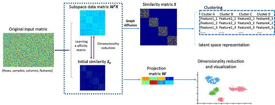
3. Locality Sensitive Discriminative Unsupervised Dimensionality Reduction

3.1. Intrinsic Structure Representation

The proposed method needs a pre-defined affinity matrix S as the initial graph. While learning the affinity values of S, we get a smaller distance by adopting the the square of Euclidean distance ${∥x_i-x_j∥}_2^2$, which is related to a larger affinity value $s_{ij}$. Thus, determining the value of $s_{ij}$ can be seen as solving the following problem:

$$\begin{array}{c}{\displaystyle \underset{{\mathbf{s}}_i^T\mathbf{1}=1,s_i\ge 0,s_{ii}=0}{min}}{\displaystyle \sum _{j=1}^n}\left({∥x_i-x_j∥}_2^2{s}_{ij}+\theta s_{ij}^2\right),\hfill \end{array}$$

(4)

where $\theta$ is the regularization parameter. The affinities are learned using a suitable $\theta$ in formula (4) so that we can get the optimal solution $s_i$ with k nonzero values, i.e., the number of neighbors k. Let us define $e_{ij}={∥x_i-x_j∥}_2^2$ and denote $e_i$ as a vector and $e_{ij}$ as j-th element; formula (4) can be simplified as

$$\begin{array}{c}{\displaystyle \underset{{\mathbf{s}}_i^T\mathbf{1}=1,s_i\ge 0,s_{ii}=0}{min}}\frac{1}{2}{∥{\mathbf{s}}_i+\frac{1}{2\theta }{e}_i∥}_2^2.\hfill \end{array}$$

(5)

According to [22], we can get the optimal affinities ${\widehat{s}}_{ij}$ as follows:

$$\begin{array}{c}{\widehat{s}}_{ij}=\left\{\begin{array}{c}\frac{e_{i,k+1}-e_{ij}}{k{e}_{i,k+1}-\sum {}_{h=1}^k{e}_{ih}},j\le k,\\ 0,j>k.\end{array}\right.\hfill \end{array}$$

(6)

Next, we define two adjacency graphs $M_s=\{X,S\}$ and $M_d=\{X,V\}$ in order to characterize the intrinsic structure of data. Among them, the elements in matrix S represent the similarity between nearby points, and the elements in matrix V represent the diversity between nearby points. We define the elements $v_{ij}$ in V as follows:

$$\begin{array}{c}{v}_{ij}=\left\{\begin{array}{c}1-s_{ij},j\le k,\\ 0,j>k.\end{array}\right.\hfill \end{array}$$

(7)

Following the above work, we still did not get a clear and simple intrinsic structure if only using similarity or diversity. Therefore, two objective functions simultaneously proposed to emphasize the local intrinsic structure. One objective function is proposed to guarantee that nearby data points should be embedded to be close to each other in the subspace and mainly focuses on preserving the similarity relationships among nearby data; the other objective function mainly focuses on the shape of a manifold and guarantees that nearby data with large distance are not embedding to be very close to each other in the subspace and effectively preserves the diversity relationships of data. By integrating this two objective functions, the local topology are guaranteed, that is to say, similarity property and diversity property of the data can be perfectly preserved. Based on the above conclusions, we employ the following objective functions to capture the local intrinsic structure:

$$\begin{array}{c}{\displaystyle \underset{W^{T}W=I}{min}}{\displaystyle \sum _{i,j=1}^n}{∥W^T{x}_i-W^T{x}_j∥}_2^2{s}_{ij},\hfill \end{array}$$

(8)

$$\begin{array}{c}{\displaystyle \underset{W^{T}W=I}{max}}{\displaystyle \sum _{i,j=1}^n}{∥W^T{x}_i-W^T{x}_j∥}_2^2{v}_{ij}.\hfill \end{array}$$

(9)

By simple algebra, we have:

$$\begin{array}{c}{\displaystyle \sum _{i,j=1}^n}{∥W^T{x}_i-W^T{x}_j∥}_2^2{s}_{ij}=tr\left(W^{T}X{L}_S{X}^{T}W\right),\hfill \end{array}$$

(10)

$$\begin{array}{c}{\displaystyle \sum _{i,j=1}^n}{∥W^T{x}_i-W^T{x}_j∥}_2^2{v}_{ij}=tr\left(W^{T}X{L}_V{X}^{T}W\right),\hfill \end{array}$$

(11)

where $L_S=D-(S+S^T)/2$ and $L_V=P-(V+V^T)/2$, $P\in R^{n\times n}$ is a diagonal matrix and its entries are column sum of V. Furthermore, in order to consider the global geometric structure information of data, we introduce the third objective function, i.e., preserving as much information as possible by maximizing overall variance of the input data. Then, inspired by LDA, we can construct a concise discriminant criterion by combining the three objective functions, which contain both local and global geometrical structures information for dimensionality reduction:

$$\begin{array}{c}{\displaystyle {\displaystyle \underset{W}{min}}\frac{tr\left(W^{T}X\left(L_S-\beta L_V\right)X^{T}W\right)}{tr\left(W^{T}XH{X}^{T}W\right)},}\hfill \\ s.t.W^{T}W=I.\hfill \end{array}$$

(12)

Bringing the definitions of $L_S$ and $L_V$ into Equation (12), we have:

$$\begin{array}{c}tr\left(W^{T}X\left(L_S-\beta L_V\right)X^{T}W\right)={\displaystyle \sum _{i,j=1}^n}{∥W^T{x}_i-W^T{x}_j∥}_2^2{s}_{ij}-\beta {\displaystyle \sum _{i,j=1}^n}{∥W^T{x}_i-W^T{x}_j∥}_2^2{v}_{ij}\hfill \\ =\left(1+\beta \right){\displaystyle \sum _{i,j=1}^n}{∥W^T{x}_i-W^T{x}_j∥}_2^2{s}_{ij}-\beta {\displaystyle \sum _{i=1}^n}{\displaystyle \sum _{j=1}^k}{∥W^T{x}_i-W^T{x}_j∥}_2^2.\hfill \end{array}$$

(13)

According to the definition of $s_{ij}$, when $j>k$, we have $s_{ij}=0$. Therefore, ${\displaystyle \sum _{i,j=1}^n}{∥W^T{x}_i-W^T{x}_j∥}_2^2{s}_{ij}$ models the local geometric structure, while ${\displaystyle \sum _{i=1}^n}{\displaystyle \sum _{j=1}^k}{∥W^T{x}_i-W^T{x}_j∥}_2^2$ represents the total scatter in the local region. Thus, we call this model locality sensitive discriminative unsupervised dimensionality reduction.

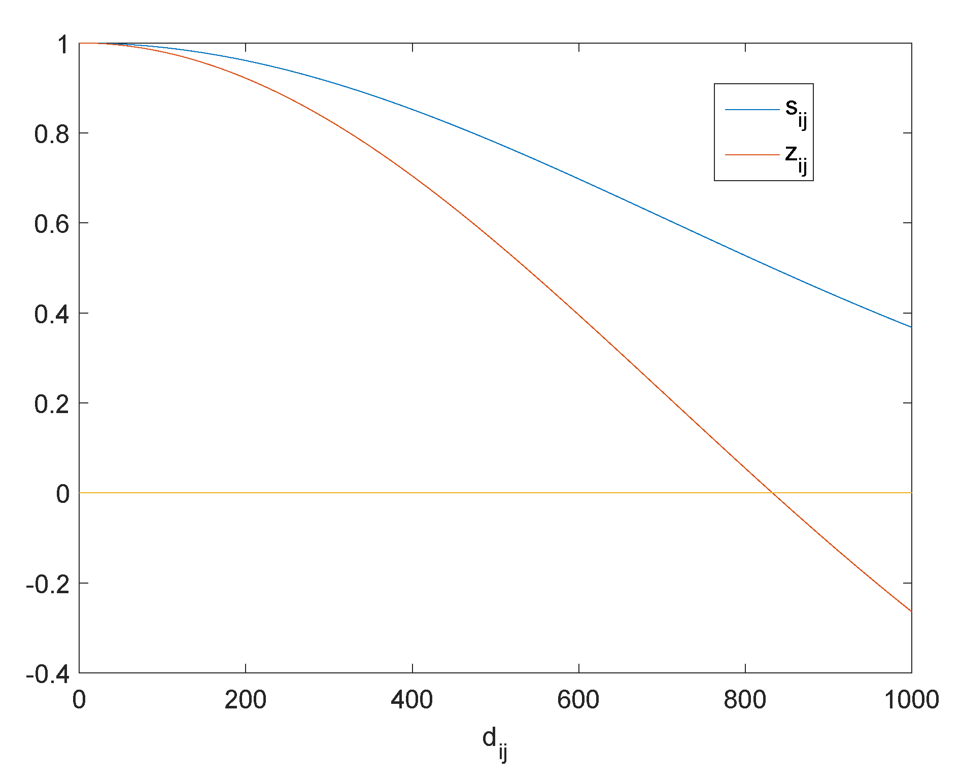
3.2. Analysis of Optimal Graph Learning

When the data contain a large number of noise samples, the similarity matrix S obtained by Equation (6) is virtually impossible to be the ideal state. The desired situation is that we map the data to a low-dimensional subspace in which the elements of similarity matrix within a cluster is nonzero and evenly distributed while the values of elements between clusters are zero. Based the above considerations, we adopt a novel and feasible way to achieve the desired state:

$$\begin{array}{c}{\displaystyle {\displaystyle \underset{W,S}{min}}\frac{tr\left(W^{T}X\left(L_S-\beta L_V\right)X^{T}W\right)}{tr\left(W^{T}XH{X}^{T}W\right)}+\theta {∥S∥}_F^2}\hfill \\ s.t.\forall i,{\mathbf{s}}_i^T\mathbf{1}=1,0\le s_{ij}\le 1,W^{T}W=I,rank\left(L_S\right)=n-c.\hfill \end{array}$$

(14)

In order to exclude the situation of trivial solution, we add the regularization term $\theta {∥S∥}_F^2$. The first and second constraints are added according to the definition of graph weights, which is defined for a vertex as the sum of the distance between one vertex and the members and is non-negative. In addition, we also add the rank constraint to the problem. If S is non-negative, the Laplacian matrix has a significant property:

Theorem 1.

A graph S with $s_{ij}\ge 0(\forall i,j)$ has c connected components if and only if the algebraic multiplicity of eigenvalue 0 for the corresponding Laplacian matrix $L_S$ is c [26].

Theorem 1 reveals that, when $rank\left(L_S\right)=n-c$, the obtained graph could distinctly divide the data set into exactly c clusters based on the block diagonal structure of similarity matrix S. It is worth mentioning that Equation (14) can simultaneously learn the projection matrix W and the similarity matrix S, which is significantly different from previous works. However, it is hard to tackle it directly, especially when there are several strict constraints. In order to solve the question, an iterative optimization algorithm is proposed.

4. Optimization

4.1. Determine the Value of S, W, F

Without loss of generality, suppose ${\sigma }_i\left(L_S\right)$ is the i-th smallest eigenvalue of $L_S$. It is clearly seen that ${\sigma }_i\left(L_S\right)\ge 0$ since $L_S$ is positive semi-definite. Then, if $\lambda$ is big enough, Equation (14) can be rewritten as:

$$\begin{array}{c}{\displaystyle {\displaystyle \underset{W,S}{min}}\frac{tr\left(W^{T}X\left(L_S-\beta L_V\right)X^{T}W\right)}{tr\left(W^{T}XH{X}^{T}W\right)}+\theta {∥S∥}_F^2+2\lambda {\displaystyle \sum _{i=1}^c}{\sigma }_i\left(L_S\right)}\hfill \\ s.t.\forall i,{\mathbf{s}}_i^T\mathbf{1}=1,0\le s_{ij}\le 1,W^{T}W=I.\hfill \end{array}$$

(15)

Hyperparameter $\lambda$ here can be used to trade balance between the rank of the graph Laplacian and consistency of the data structure. The rank constraint of the graph Laplacian is usually satisfied with a large enough $\lambda$. Meanwhile, given a rank-enforcing matrix $F\in R^{n\times c}$, suppose that node i is assigned a function value as ${\mathrm{f}}_i\in R^{1\times c}$. According to the Ky Fan’s Theorem [27], the rank constraint term in Equation (15) can be seen as the optimization of the smallest c eigenvalues of the Laplacian matrix. Thus, we can transform Equation (15) into the following form:

$$\begin{array}{c}{\displaystyle {\displaystyle \underset{W,S,F}{min}}\frac{tr\left(W^{T}X\left(L_S-\beta L_V\right)X^{T}W\right)}{tr\left(W^{T}XH{X}^{T}W\right)}+\theta {∥S∥}_F^2+2\lambda tr\left(F^T{L}_{S}F\right),}\hfill \\ s.t.\forall i,{\mathbf{s}}_i^T\mathbf{1}=1,0\le s_i\le 1,W^{T}W=I,F^{T}F=I.\hfill \end{array}$$

(16)

When S and F are fixed, problem (16) can be rewritten as:

$$\begin{array}{c}{\displaystyle {\displaystyle \underset{W}{min}}\frac{tr\left(W^{T}X\left(L_S-\beta L_V\right)X^{T}W\right)}{tr\left(W^{T}XH{X}^{T}W\right)}}\hfill \\ s.t.W^{T}W=I.\hfill \end{array}$$

(17)

We can use the iterative method introduced in [28] to solve W from Equation (17), and the Lagrangian function is constructed according to Equation (17):

$$\begin{array}{c}{\displaystyle L\left(W,\eta \right)=\frac{tr\left(W^{T}X\left(L_S-\beta L_V\right)X^{T}W\right)}{tr\left(W^{T}XH{X}^{T}W\right)}-\eta tr\left(W^{T}W-I\right),}\hfill \end{array}$$

(18)

where $\eta$ is a scalar. Then, taking the derivative of W and letting the result be zero, we have

$$\begin{array}{c}{\displaystyle \left(X\left(L_S-\beta L_V\right)X^T-\frac{tr\left(W^{T}X\left(L_S-\beta L_V\right)X^{T}W\right)}{tr\left(W^{T}XH{X}^{T}W\right)}XH{X}^T\right)W=\tilde{\eta }W,}\hfill \end{array}$$

(19)

where $\tilde{\eta }=\eta tr\left(W^{T}XH{X}^{T}W\right)$. The optimal solution of W in Equation (19) is formed by the m eigenvectors corresponding to the m smallest eigenvalues of the matrix:

$$\begin{array}{c}{\displaystyle \left(X\left(L_S-\beta L_V\right)X^T-\frac{tr\left(W^{T}X\left(L_S-\beta L_V\right)X^{T}W\right)}{tr\left(W^{T}XH{X}^{T}W\right)}XH{X}^T\right).}\hfill \end{array}$$

(20)

When W and S are fixed, problem (16) becomes

$$\begin{array}{c}{\displaystyle {\displaystyle \underset{F}{min}}2\lambda tr\left(F^T{L}_{S}F\right)}\hfill \\ s.t.F^{T}F=I.\hfill \end{array}$$

(21)

Since $\lambda$ is a constant, the optimal solution of rank-enforcing matrix F in Equation (21) is composed of c eigenvectors, which are derived from c smallest eigenvalues of Laplacian matrix $L_S$.

When we fix W and F, problem (16) was written as:

$$\begin{array}{c}{\displaystyle {\displaystyle \underset{S}{min}}{\displaystyle \sum _{i,j=1}^n}\left(\frac{\left(1+\beta \right){∥W^T{x}_i-W^T{x}_j∥}_2^2{s}_{ij}}{tr\left(W^{T}XH{X}^{T}W\right)}+\theta s_{ij}^2+\lambda {∥{\mathbf{f}}_i-{\mathbf{f}}_j∥}_2^2{s}_{ij}\right)}\hfill \\ s.t.\forall i,{\mathbf{s}}_i^T\mathbf{1}=1,0\le s_{ij}\le 1.\hfill \end{array}$$

(22)

Note that problem (22) can be solved independently for different ${\mathbf{s}}_i$, so that the following problem can be solved separately for each i:

$$\begin{array}{c}{\displaystyle {\displaystyle \underset{{\mathbf{s}}_{\mathbf{i}}}{min}}{\displaystyle \sum _{i=1}^n}({\Gamma }_{ij}{s}_{ij}+\theta s_{ij}^2+\lambda {\Psi }_{ij}{s}_{ij})}\hfill \\ s.t.\forall i,{\mathbf{s}}_i^T\mathbf{1}=1,0\le s_{ij}\le 1,\hfill \end{array}$$

(23)

where ${\Gamma }_{ij}=\frac{\left(1+\beta \right){∥W^T{x}_i-W^T{x}_j∥}_2^2}{tr\left(W^{T}XH{X}^{T}W\right)}$ and ${\Psi }_{ij}={∥{\mathbf{f}}_i-{\mathbf{f}}_j∥}_2^2$. Then, Equation (23) can be rewritten as:

$$\begin{array}{c}{\displaystyle {\displaystyle \underset{{\mathbf{s}}_i}{min}}{∥{\mathbf{s}}_i+\frac{1}{2\theta }({\Gamma }_i+\lambda {\Psi }_i)∥}_2^2}\hfill \\ s.t.\forall i,{\mathbf{s}}_i^T\mathbf{1}=1,0\le s_{ij}\le 1.\hfill \end{array}$$

(24)

Thus, Equation (24) can be solved easily with a close form solution. Denote vector ${\mathbf{d}}_i\in R^{n\times 1}$ with $d_{ij}={\Gamma }_{ij}+\lambda {\Psi }_{ij}$. For each i, Lagrange functions can be obtained:

$$\begin{array}{c}\mathrm{L}(W,\varsigma ,{\gamma }_i^{})=\frac{1}{2}{∥{\mathbf{s}}_i+\frac{1}{2\theta }{\mathbf{d}}_i∥}_2^2-\varsigma ({\mathbf{s}}_i^T\mathbf{1}-1)-{\gamma }_i^T{\mathbf{s}}_i,\hfill \end{array}$$

(25)

where $\varsigma$ and ${\gamma }_i^T\ge 0$ are the Lagrangian multipliers. Take a partial derivative for each ${\mathbf{s}}_i$ and set it to zero; then, according to K.K.T. conditions:

$$\begin{array}{c}{\left({\mathbf{s}}_i\right)}_j-{\left({\mathbf{d}}_i\right)}_j+\varsigma -{\gamma }_i^{}=0,\hfill \\ {\left({\mathbf{s}}_i\right)}_j\ge 0,\hfill \\ {\gamma }_i^{}\ge 0,\hfill \\ {\left({\mathbf{s}}_i\right)}_j{\gamma }_i^{}\ge 0,\hfill \\ {\mathbf{s}}_i^T\mathbf{1}-1=0.\hfill \end{array}$$

(26)

Then, we can obtain ${\mathbf{s}}_i$ that should be:

$$\begin{array}{c}{s}_{ij}={[-\frac{1}{2{\theta }_i}{\mathbf{d}}_i+\varsigma ]}_{+}.\hfill \end{array}$$

(27)

4.2. Approach to Determine the Initial Value of $\theta$, $\lambda$

In actual experiments, regularization parameters are difficult to tune because their values may range from zero to infinity. In this section, we propose an efficient way to determine the regularization parameter $\theta$ and $\lambda$ as follows:

$$\begin{array}{c}\lambda =\theta =\frac{1}{n}{\displaystyle \sum _{j=1}^n}[\frac{k}{2}{d}_{i,k+1}-\frac{1}{2}{\displaystyle \sum _{j=1}^k}{d}_{ij}].\hfill \end{array}$$

(28)

k is a pre-defined parameter. In this way, we only need to set the number of neighbors we prefer rather than setting two hyper-parameters of $\theta$ and $\lambda$. The number of neighbors is usually easy to set according to the number of samples and locality of the data set. The rationality of deciding $\theta$ and $\lambda$ using the distance gaps between k-th neighbor and $(k+1)$-th neighbor lies in the fact that, to achieve a desired similarity where the top k-neighbor similarities are kept and the rest are set to zeros, we should approximately achieve

$$\begin{array}{c}\frac{k}{2}{d}_{ik}-\frac{1}{2}{\displaystyle \sum _{j=1}^k}{d}_{ij}<{\theta }_i\le \frac{k}{2}{d}_{i,k+1}-\frac{1}{2}{\displaystyle \sum _{j=1}^k}{d}_{ij},\hfill \end{array}$$

(29)

where $d_{i1},d_{i2},...,d_{in}$ are sorted in ascending order. If we set the inequality to equality, we can get an estimation of $\theta$:

$$\begin{array}{c}\theta \sim \frac{1}{n}{\displaystyle \sum _{j=1}^n}[\frac{k}{2}{d}_{i,k+1}-\frac{1}{2}{\displaystyle \sum _{j=1}^k}{d}_{ij}].\hfill \end{array}$$

(30)

Similarly, $\lambda$ is set to be equal to $\theta$ as follows:

$$\begin{array}{c}\lambda =\theta \sim \frac{1}{n}{\displaystyle \sum _{j=1}^n}[\frac{k}{2}{d}_{i,k+1}-\frac{1}{2}{\displaystyle \sum _{j=1}^k}{d}_{ij}].\hfill \end{array}$$

(31)

Since these two parameters control the regularization strength, we adaptively update the parameters during each iteration:

• When the connected components are insufficient, i.e., the number of zero eigenvalues is smaller than c, we multiply $\lambda$ by 2.
• The number of connected components could be overrun, i.e., the number of zero eigenvalues is larger than c. We divide $\lambda$ by 2.
• If the graph has exact c connected components, then we stop the algorithm in this case and return the result.

The detailed steps are summarized in Algorithm 1.

Algorithm 1 Framework of the LSDUDR method.

Require: Data $X\in R^{d\times n}$, cluster number c, projection dimension m.  Initialize S and V according to Equations (6) and (7). Initialize parameter $\theta$ and $\lambda$ by the Equation (28).  If algorithm 1 not converge:  repeat   1. Construct the Laplacian matrix $L_S=D-(S+S^T)/2$ and $L_V=P-(V+V^T)/2$.   2. Calculate F, columns of F are c eigenvectors of $L_S$ and are derived from the c samllest   eigenvalues.   3. Calculate the projection matrix W by the m eigenvectors corresponding to the m smallest   eigenvalues of the matrix: $$\begin{array}{c}{\displaystyle \left(X\left(L_S-\beta L_V\right)X^T-\frac{tr\left(W^{T}X\left(L_S-\beta L_V\right)X^{T}W\right)}{tr\left(W^{T}XH{X}^{T}W\right)}XH{X}^T\right).}\hfill \end{array}$$   4. Compute S by updating ${\mathbf{s}}_i$ according to Equation (27).   5. Calculate the number of connected components of the graph, if it is smaller than c, then multiply   $\lambda$ by 2; if larger than c, then divide $\lambda$ by 2.  until Convergence  End if  return  Projection matrix $W\in R^{d\times m}$ and similarity matrix $S\in R^{n\times n}$.

5. Discussion

5.1. Analysis

As previously discussed, LSDUDR represents the local intrinsic structure of data set based on Equations (8) and (9). Then, we integrate the two objective functions as follows:

$$\begin{array}{c}{\displaystyle \sum _{i,j=1}^n}{∥W^T{x}_i-W^T{x}_j∥}_2^2{s}_{ij}-\beta {\displaystyle \sum _{i,j=1}^n}{∥W^T{x}_i-W^T{x}_j∥}_2^2{v}_{ij}\hfill \\ ={\displaystyle \sum _{i=1}^n}{\displaystyle \sum _{j=1}^k}{∥W^T{x}_i-W^T{x}_j∥}_2^2\left(s_{ij}+\beta s_{ij}-1\right)\hfill \\ ={\displaystyle \sum _{i,j=1}^n}{∥W^T{x}_i-W^T{x}_j∥}_2^2{z}_{ij},\hfill \end{array}$$

(32)

where the elements $z_{ij}$ are defined as follows:

$$\begin{array}{c}{z}_{ij}=\left\{\begin{array}{c}{s}_{ij}+\beta s_{ij}-1,j\le k,\\ 0,j>k.\end{array}\right.\hfill \end{array}$$

(33)

It is easy to see that Equation (32) is very similar to Equation (8). However, they are completely different when they express the intrinsic geometrical structure of the data. Without loss of generality, we set the weight elements $s_{ij}$ in Equation (8) as a heat kernel function. Figure 2 shows their weight change process with a distance between two points $x_i$ and $x_j$.

As we know, the real-world data are usually unbalanced and complex, thus some points may be distributed in sparse areas while other data points are distributed in compact areas. As shown in Figure 2, $z_{ij}$ is positive for data points in compact regions, thus Equation (32) maps these data points to be very close in the subspace, and mainly preserves the similarity of data. If data points lie in sparse regions, $z_{ij}$ is negative, and Equation (32) mainly characterizes diversity of data in this case, i.e., the shape of a manifold structure. However, the difference among points in a neighborhood is not considered in Equation (8), and always projects the neighborhood points to be close into subspace, which ignores the intrinsic geometrical structure of data.

It is noteworthy that three updating rules are included in the proposed algorithm, which are computationally efficient. In fact, [29] has already proven the convergence of the alternative optimization method. In our algorithm, the main cost lies in each iteration being the eigen-decomposition step for Equations (7) and (21). The time computational complex of the proposed method is $O\left((d^{2}m+n^{2}c)t\right)$, where t is the number of iterations.

5.2. Convergence Study

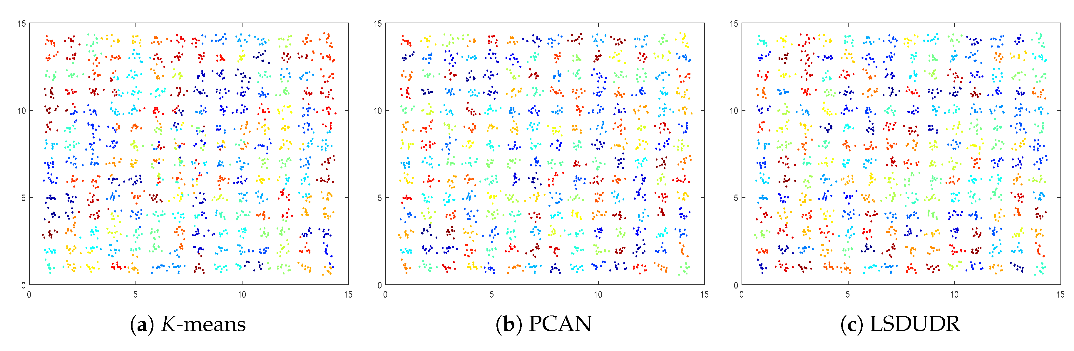
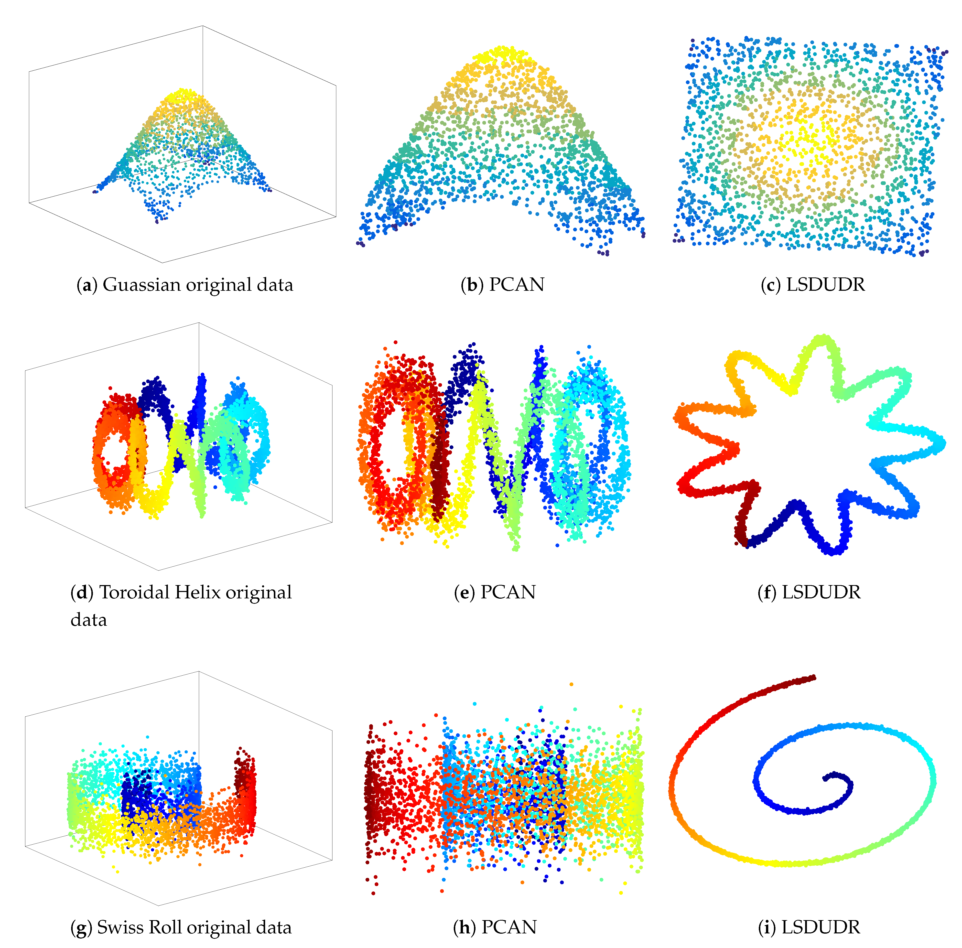
The method proposed by Algorithm 1 can be used to find a locally optimal solution of problem (14). The convergence of Algorithm 1 is given through Theorem (2).

Theorem 2.

The alternate updating rules in Algorithm 1 monotonically decrease the objective function value of optimization problem (14) in each iteration until convergence.

Proof. 

In the procedure of iteration, we get the global optimal selective matrix $W_{t+1}$ by solving optimization problem $W_{t+1}=arg{\displaystyle \underset{W^{T}W=I}{min}}\frac{tr\left(W^{T}X\left(L_S-\beta L_V\right)X^{T}W\right)}{tr\left(W^{T}XH{X}^{T}W\right)}$. As a result, we have the following inequality:

$$\begin{array}{c}\frac{tr\left(W_{t+1}^{T}X\left(L_S-\beta L_V\right)X^T{W}_{t+1}^T\right)}{tr\left(W_{t+1}^{T}XH{X}^T{W}_{t+1}^T\right)}\le \frac{tr\left(W_t^{T}X\left(L_S-\beta L_V\right)X^T{W}_t^T\right)}{tr\left(W_t^{T}XH{X}^T{W}_t^T\right)}.\hfill \end{array}$$

(34)

Since variable $F_{t+1}$ is updated by solving problem $F_{t+1}^T=arg{\displaystyle \underset{F^{T}F=I}{min}}2\lambda tr\left(F_t^{T}L{F}_t^T\right)$, we obtain the following inequality:

$$\begin{array}{c}tr\left(F_{t+1}^{T}L{F}_{t+1}^T\right)\le tr\left(F_t^{T}L{F}_t^T\right).\hfill \end{array}$$

(35)

Consequently, we have the following inequality:

$$\begin{array}{c}\frac{tr\left(W_{t+1}^{T}X\left(L_S-\beta L_V\right)X^T{W}_{t+1}^T\right)}{tr\left(W_{t+1}^{T}XH{X}^T{W}_{t+1}^T\right)}+tr\left(F_{t+1}^{T}L{F}_{t+1}^T\right)\le \frac{tr\left(W_t^{T}X\left(L_S-\beta L_V\right)X^T{W}_t^T\right)}{tr\left(W_t^{T}XH{X}^T{W}_t^T\right)}+tr\left(F_t^{T}L{F}_t^T\right).\hfill \end{array}$$

(36)

In addition, K.K.T. conditions (26) illustrate that the converged solution of Algorithm 1 is at least a stationary point of Equation (25). Because the updating of weights matrix $S_{t+1}\in R^{n\times n}$ can be divided into n independently sub-optimization problem with respect to n-dimensional vector. Consequently, the objective function value of optimization problem (14) decreases monotonically in each iteration until the algorithm convergence. □

6. Experiment

In the experiment, the following two metrics are used to evaluate the performance of the proposed LSDUDR algorithm: Accuracy (ACC) and Normalized Mutual Information (NMI) [30]. Accuracy is defined as

$$\begin{array}{c}ACC=\frac{{\displaystyle \sum _{i=1}^n}\delta \left(t_i,map\left(t_i^g\right)\right)}{n},\hfill \end{array}$$

(37)

where $t_i$ is the label of the clustering result and $t_i^g$ is the known label of $x_i$. $map\left(t_i^g\right)$ is the optimal mapping function that permutes the label set of the clustering results and the known label set of samples. $\delta \left(t_i,map\left(t_i^g\right)\right)$ is an indicator function. Normalized Mutual Information is defined as

$$\begin{array}{c}NMI=\frac{{\displaystyle \sum _{i,j=1}^c}{t}_{ij}log\frac{n\times t_{ij}}{t_i{\widehat{t}}_j}}{\sqrt{\left({\displaystyle \sum _{i=1}^c}{t}_{i}log\frac{t_i}{n}\right)\left({\displaystyle \sum _{j=1}^c}{\widehat{t}}_{j}log\frac{{\widehat{t}}_j}{n}\right)}},\hfill \end{array}$$

(38)

where $t_i$ is the number of samples in the i-th cluster $C_i$ according to clustering results and ${\widehat{t}}_j$ is the number of samples in the j-th ground truth class $G_j$. $t_{ij}$ is the number of overlap between $C_i$ and $G_j$.

We compare the performance of LSDUDR with K-Means [31], Ratio Cut [32], Normalized Cut [33] and PCAN methods, since they are closely related to LSDUDR, i.e., the information contained in the eigenvectors of an affinity matrix is used to detect the similarity. We made comparisons with Ratio Cut, Normalized Cut to show that LSDUDR can effectively mitigate the influence of outliers by inducing robustness and adaptive neighbors. To emphasize the importance of describing the intrinsic manifold structure, we compared the results of PCAN with LSDUDR which concatenates to uncover the intrinsic topology structures of data by proposing two objective functions and performs discriminatively embedded K-Means clustering.

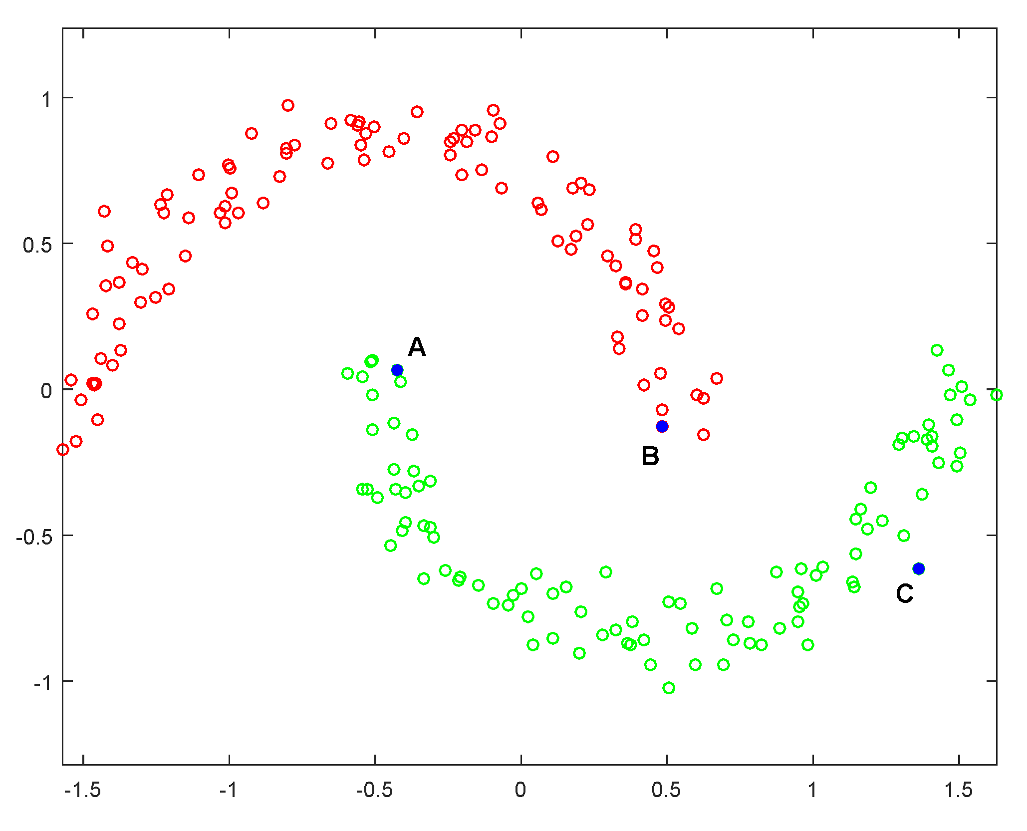
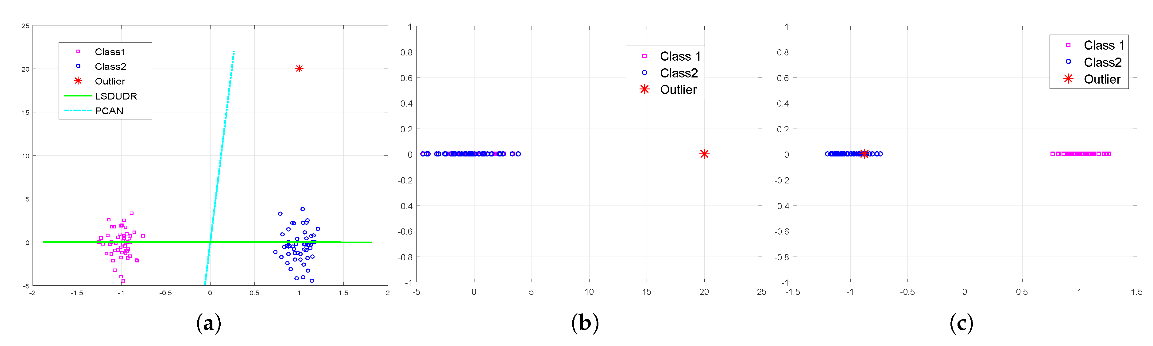
6.1. Experiment on the Synthetic Data Sets

To verify the robust performances and strong discriminating power of the proposed LSDUDR, two simple synthetic examples (two-Gaussian and multi-cluster data) are given in this experiment.

In this first synthetic data set, we deliberately set a point away from the two-Gaussian distribution as an outlier so that a one-dimensional linear manifold representation was obtained to clearly divide two clusters. LSDUDR and PCAN were demonstrated on the synthetic examples respectively and the results are shown in Figure 3. It is clear that one cluster shown in pink almost submerges in another one as blue in the one-dimensional representation using PCAN, while it is separated distinctly out using LSDUDR, so we can conclude that LSDUDR has more discriminating power than PCAN. Furthermore, LSDUDR is less sensitive to outliers than PCAN because the objective function of LSDUDR will bring a heavy penalty to two points when they are embedded to be close in the subspace but with large distance in the origin space.

The second synthetic data set is a multi-cluster data, which contains 196 randomly generated clusters that are distributed in a spherical manner. We compared LSDUDR with K-means and PCAN. Due to the fact that K-means is sensitive to initialization [34], we repeatedly run K-means 100 times and use the minimal K-means objective value as the result. To be fair, the parameters of PCAN are adjusted to report the best performance of PCAN. As for LSDUDR, we run LSDUDR once to generate a clustering result and use it as initialization for K-means and report the best performance.

Table 1. Compare results on multi-cluster synthetic data sets.

Methods	ACC%	Minimal K-Means Objective
K-Means	66.94	336.46
PCAN	98.62	107.33
LSDUDR	99.49	106.21

and Figure 4 show the experiment results of LSDUDR and other two algorithms on multi-cluster data. As can be seen from Table 1, LSDUDR obtained better performance than those of other methods according to the the minimal K-means objective value and clustering accuracy. Thus, LSDUDR has stronger discriminating power than PCAN and K-means especially when the data distribution is complex.

6.2. Experiment on Low-Dimensional Benchmark Data Sets

In this subsection, we evaluate the performance of the proposed LSDUDR on ten low-dimensional benchmark data sets with comparison to four related methods, including K-Means, Ratio Cut, Normalized Cut and PCAN methods. Description of these data sets is summarized in

Table 2. Specifications of the data sets.

Data Set	#Classes (c)	#Data Points (n)	#Dimensions (d)
Spiral	3	312	2
Pathbased	3	300	2
Compound	6	399	2
Movements	15	360	90
Iris	3	150	4
Cars	3	392	8
Glass	6	214	9
Vote	2	435	16
Diabetes	2	768	8
Dermatology	6	366	34

, including four synthetic data sets and six University of CaliforniaIrvine (UCI) datasets [35]. In low-dimensional data, we set the projection dimension in PCAN and LSDUDR to be $c-1$. For the methods that require a fixed input data graph, we use the self-turn Gaussian method [34,36] to build the graph. For the methods involving K-Means to extract the clustering labels, we repeatedly ran K-Means 100 times with the same settings and chose the best performance. As for PCAN and LSDUDR, we only ran it once and reported the result directly from the learned graph. The experimental results are shown in

Table 3. ACC(%) on low-dimensional benchmark data sets.

ACC%	K-Means	RatioCut	NormalizedCut	PCAN	LSDUDR
Spiral	33.97	99.68	99.68	100	100
Pathbased	74.33	77.33	76.67	87.00	87.00
Compound	80.20	76.69	65.91	78.95	88.22
Movements	10.56	5.83	10.56	56.11	55.56
Iris	66.67	68.00	66.39	77.33	92.00
Cars	44.90	53.27	47.70	48.98	58.42
Glass	52.21	36.45	51.87	49.07	52.80
Vote	83.45	61.61	83.68	67.36	85.75
Diabetes	56.02	64.71	61.98	58.46	65.10
Dermatology	85.25	54.92	93.72	94.81	95.90

and

Table 4. NMI(%) on low-dimensional benchmark data sets.

NMI%	K-Means	RatioCut	NormalizedCut	PCAN	LSDUDR
Spiral	12.52	98.35	98.35	100	100
Pathbased	51.33	54.96	53.10	75.63	79.27
Compound	79.74	71.60	66.32	77.48	85.16
Movements	44.11	15.85	44.91	84.95	84.17
Iris	61.68	61.3	59.05	61.85	77.52
Cars	39.10	21.61	39.06	39.03	39.39
Glass	35.83	35.33	34.88	35.76	35.90
Vote	36.58	30.17	35.66	35.23	39.37
Diabetes	52.67	50.02	61.98	64.01	68.10
Dermatology	85.20	41.24	88.43	91.83	93.53

.

In this experiment, we can observe that PCAN and LSDUDR are much better than those of fixed graph-based methods. This observation confirms that separation of graph construction and dimensionality reduction leads the similarity matrix to not being able to be fully relied on and the experimental results will seriously deteriorate. In addition, LSDUDR outperforms other methods in nine data sets on account of preserving locality structure among data.

6.3. Embedding of Noise 3D Manifold Benchmarks

To confirm the ability of robustly characterizing the manifold structure of LSDUDR, we use three typical 3D manifold benchmark data sets [37], i.e., Guassian, Toroidal Helix and Swiss Roll. In this experiment, we tried to map these 3D manifold benchmarks to 2D in order to find out a low-dimensional embedding but with the most manifold structure information. The experimental results are shown in Figure 5.

Under the same conditions, PCAN method is also tested for comparison. Figure 5 shows the 2D embedding results of PCAN and LSDUDR which each row is related to on the manifold benchmark. It is obvious that PCAN did not find a suitable projection direction. This is because PCAN only considers the similarity between data points, which is not enough to characterize the intrinsic structure of data and even causes the destruction of a manifold structure. However, LSDUDR considers both similarity and diversity of the data set, and thus has strong sensitivity to local topology of data.

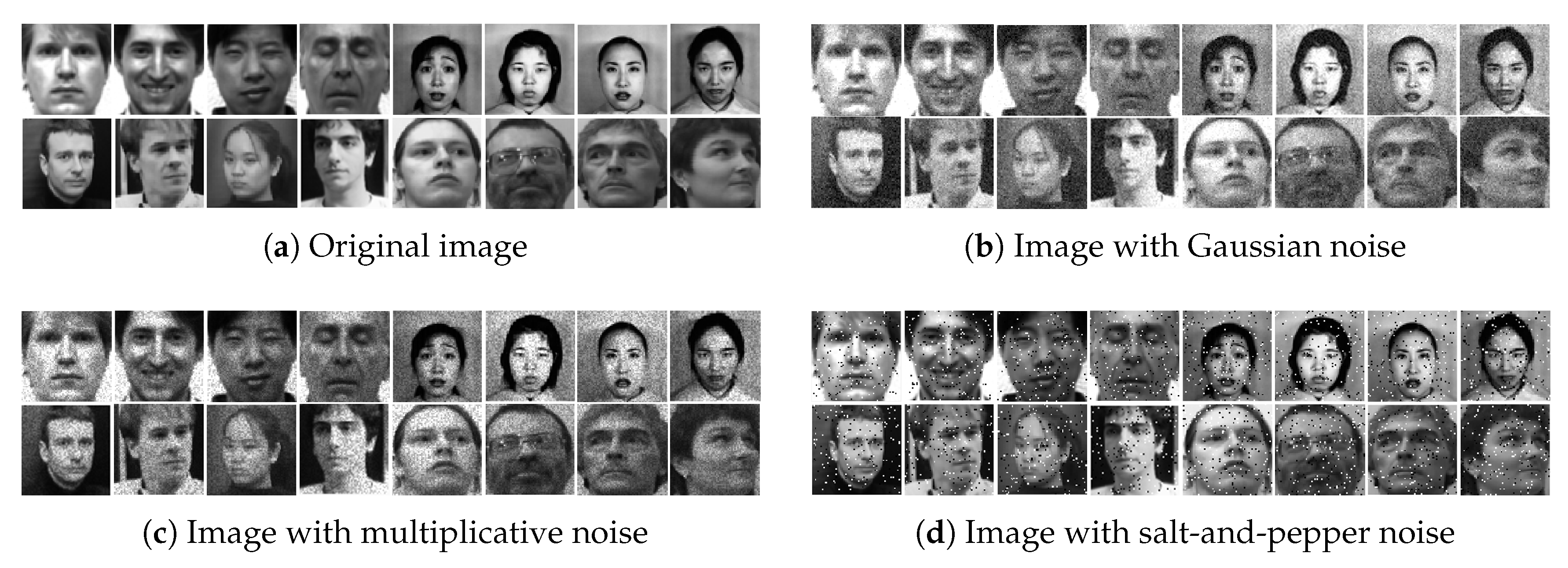
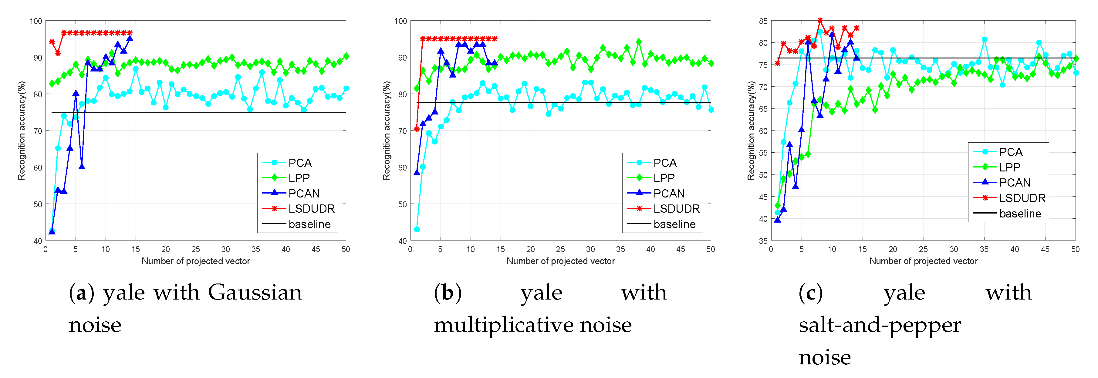
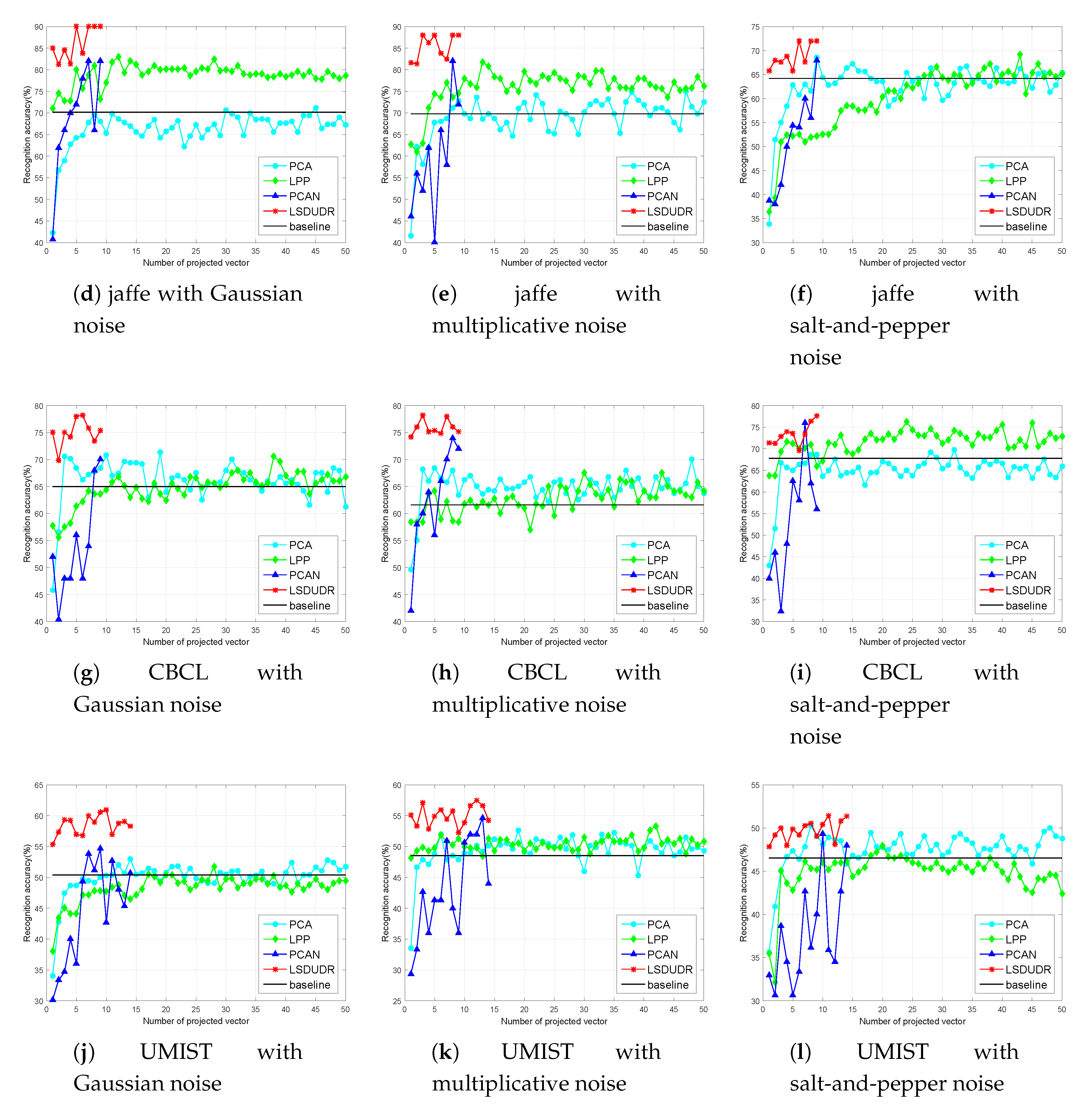
6.4. Experiment on the Image Data Sets

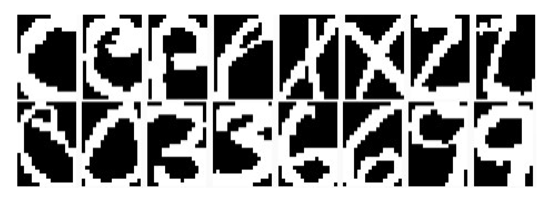
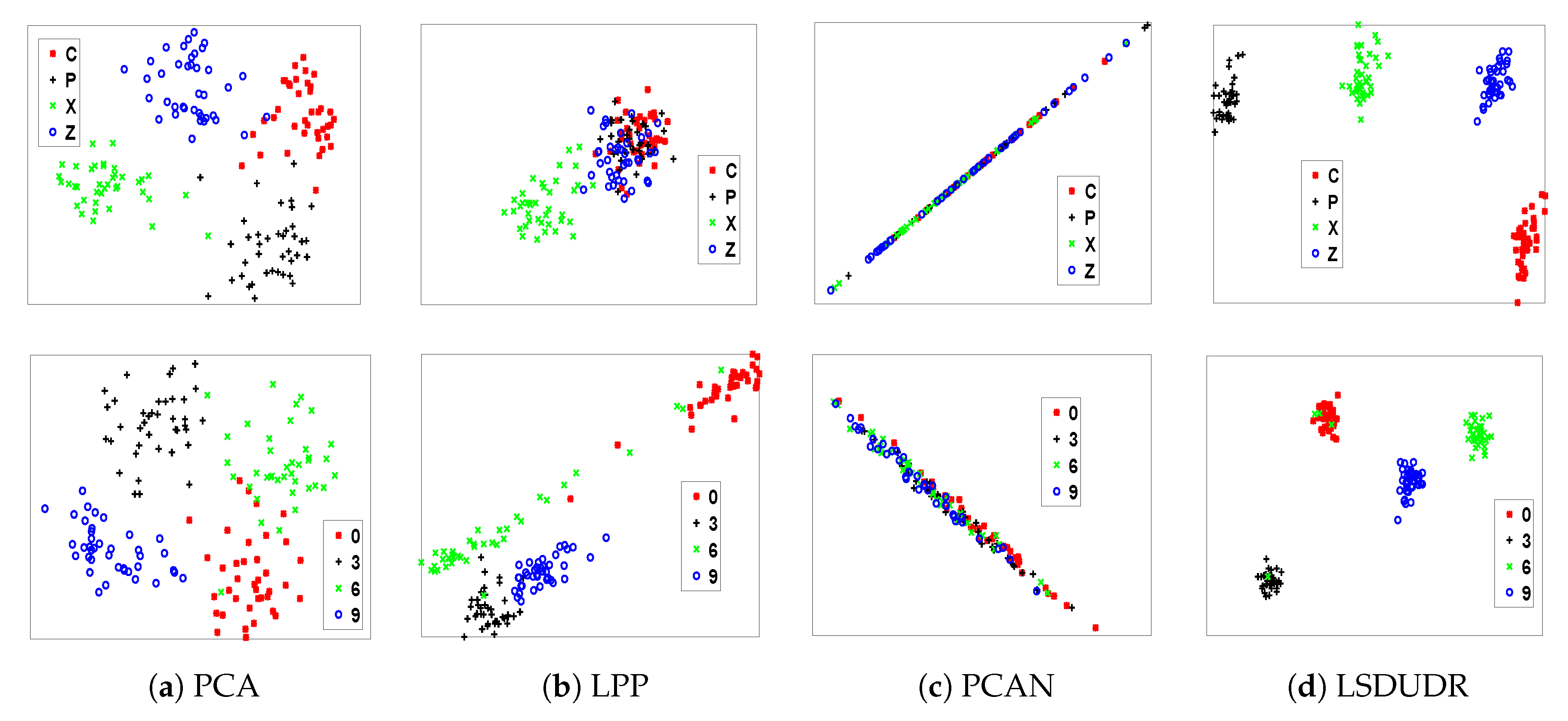
6.4.1. Visualization for Handwritten Digits

To further test the low-dimensional embedding applicability of the proposed LSDUDR algorithm, another experiment is carried out on a Binary Alphadigits data set [38], as shown in Figure 6. We select four letters (“C”, “P”, “X”, “Z”) and four digits (“0”, “3”, “6”, “9”) from the Binary Alphadigits data set, which comprises binary digits from “0” to “9” and capital “A” to “Z”. The embedding results are drawn in Figure 7.

It can be seen from Figure 7a,b that there are overlaps in clusters of “C”, “P” and “Z”, digits “0” and “6” when we use PCA and LPP. In addition, worse results are obtained from PCAN and it is shown in Figure 7c that almost all points are tangled for all clusters. However, for LSDUDR, results in Figure 7d show that classes are separated clearly, which reflects that diversity plays an important role in representing the intrinsic structure of data.

6.4.2. Face Benchmark Data Sets

We use four image benchmark data sets in this section for experiments on projection, since these data typically have high dimensionality. We summarize the four face image benchmark data sets in

Table 5. The description of the face image benchmark data sets.

Data Sets	#Classes (c)	#Data Points (n)	#Dimensions (d)
YaleA	15	165	3456
Jaffe	10	213	1024
CBCI	120	840	7668
UMIST	120	840	768

. To study the data-adaptiveness and noise-robustness of the proposed LSDUDR algorithm, we use a range of data sets contaminated by different kinds of noise based on the face data sets, as shown in Figure 8. Similar to the above-mentioned experiment, three algorithms, including PCAN, PCA and LPP, are used for comparison.

The experimental results about face benchmark data sets are shown in Figure 9, from which we get a convincing observation that the experimental results obtained by adaptive graph learning algorithms are usually more outstanding, especially when the dimensionality of projection space increases. This is because adaptive graph learning algorithms can use the embedded information that are obtained in the previous step to update the similarity matrix, hence the dimensionality reduction results are more accurate. In addition, we observe that PCA and LPP are more sensitive to the dimensionality of embedded space while the curve of LSDUDR is basically stable with the change of dimensionality. Furthermore, LSDUDR is capable of projecting the data into a subspace with a relatively small dimension $c-1$; such subspace with low dimensionality obtained by our method would be even better than the subspaces obtained by PCA and LPP with higher dimensionality. It indicates that local topology and geometrical properties were taken into account for the similarity and diversity of data when using LSDUDR, and thus have better performance and achieved higher accuracy than PCAN when the images reserve sufficient spatial information.

7. Conclusions

In this paper, a novel adaptive graph learning method (LSDUDR) is proposed from a new perspective by integrating a similarity graph and diversity graph to learn a discriminative subspace where data can be easily separated. Meanwhile, LSDUDR performs dimensionality reduction and local structure learning simultaneously based on the high quality Laplacian matrix. Different from previous graph-based models, LSDUDR constructs two adjacency graphs that could represent the intrinsic structure of data well in learning the local sensitivity of the data. Furthermore, LSDUDR doesn’t require other clustering methods to obtain cluster indicators but extracts label information from a similarity graph or diversity graph, which adaptively updates in a reconstruction manner. We also discuss the convergence of the proposed algorithm as well as the value of trade-off parameters. Experimental results on the synthetic data, face image databases and several benchmark data illustrate the effectiveness and superiority of the proposed method.

In this paper, we focus on the scenario of construction of two adjacency graphs to represent the original structure with data similarity and diversity. Our method can be used to remove irrelevant and correlated features involved in high-dimensional feature space and convert data represented in subspaces [39]. In our future work, it is potentially interesting to extend the proposed methods to unsupervised feature selection of data points with multiview and multitask.

References

1. Everitt, B.S.; Dunn, G.; Everitt, B.S.; Dunn, G. Cluster Analysis; Wiley: Hoboken, NJ, USA, 2011; pp. 115–136. [Google Scholar]
2. Xu, R.; Wunsch, D. Survey of clustering algorithms. IEEE Trans. Neural Netw. 2005, 16, 645–678. [Google Scholar] [CrossRef] [PubMed]
3. Cheng, Q.; Zhou, H.; Cheng, J. The Fisher-Markov Selector: Fast Selecting Maximally Separable Feature Subset for Multiclass Classification with Applications to High-Dimensional Data. IEEE Trans. Pattern Anal. Mach. Intell. 2011, 33, 1217–1233. [Google Scholar] [CrossRef] [PubMed]
4. Dash, M.; Liu, H. Feature selection for clustering. In Proceedings of the Pacific-Asia Conference on Knowledge Discovery and Data Mining, Keihanna Plaza, Japan, 17–20 April 2000; pp. 110–121. [Google Scholar]
5. Ben-Bassat, M. Pattern recognition and reduction of dimensionality. Handb. Stat. 1982, 2, 773–910. [Google Scholar]
6. Wold, S.; Esbensen, K.; Geladi, P. Principal component analysis. Chemom. Intell. Lab. Syst. 1987, 2, 37–52. [Google Scholar] [CrossRef]
7. FISHER, R.A. The use of multiple measurements in taxonomic problems. Ann. Eugen. 1936, 7, 179–188. [Google Scholar] [CrossRef]
8. Hall, K.M. Anr-Dimensional Quadratic Placement Algorithm. Manag. Sci. 1970, 17, 219–229. [Google Scholar] [CrossRef]
9. Belkin, M.; Niyogi, P. Laplacian Eigenmaps for Dimensionality Reduction and Data Representation. Neural Comput. 2003, 15, 1373–1396. [Google Scholar] [CrossRef] [Green Version]
10. Luo, D.; Ding, C.; Huang, H.; Li, T. Non-negative Laplacian Embedding. In Proceedings of the 2009 Ninth IEEE International Conference on Data Mining, Miami, FL, USA, 6–9 December 2009. [Google Scholar]
11. Roweis, S.T. Nonlinear Dimensionality Reduction by Locally Linear Embedding. Science 2000, 290, 2323–2326. [Google Scholar] [CrossRef] [Green Version]
12. He, X.; Niyogi, P. Locality preserving projections. In Advances in Neural Information Processing Systems; MIT Press: Vancouver, BC, Canada, 2004; pp. 153–160. [Google Scholar]
13. Nie, F.; Xiang, S.; Zhang, C. Neighborhood MinMax Projections. In Proceedings of the International Joint Conference on Artificial Intelligence (IJCAI), Hyderabad, India, 8 January 2007; pp. 993–998. [Google Scholar]
14. Tenenbaum, J.B. A Global Geometric Framework for Nonlinear Dimensionality Reduction. Science 2000, 290, 2319–2323. [Google Scholar] [CrossRef]
15. Lu, G.F.; Jin, Z.; Zou, J. Face recognition using discriminant sparsity neighborhood preserving embedding. Knowl.-Based Syst. 2012, 31, 119–127. [Google Scholar] [CrossRef]
16. Fan, Q.; Gao, D.; Wang, Z. Multiple empirical kernel learning with locality preserving constraint. Knowl.-Based Syst. 2016, 105, 107–118. [Google Scholar] [CrossRef]
17. Pandove, D.; Rani, R.; Goel, S. Local graph based correlation clustering. Knowl.-Based Syst. 2017, 138, 155–175. [Google Scholar] [CrossRef]
18. Feng, X.; Wu, S.; Zhou, W.; Min, Q. Efficient Locality Weighted Sparse Representation for Graph-Based Learning. Knowl.-Based Syst. 2017, 121, 129–141. [Google Scholar] [CrossRef]
19. Du, L.; Shen, Y.D. Unsupervised feature selection with adaptive structure learning. In Proceedings of the 21th ACM SIGKDD International Conference on Knowledge Discovery and Data Mining, Sydney, Australia, 10–13 August 2015; pp. 209–218. [Google Scholar] [CrossRef]
20. Nie, F.; Wang, H.; Huang, H.; Ding, C. Unsupervised and semi-supervised learning via L1-norm graph. In Proceedings of the 2011 International Conference on Computer Vision, Barcelona, Spain, 6–13 November 2011. [Google Scholar] [CrossRef]
21. Gao, Q.; Liu, J.; Zhang, H.; Gao, X.; Li, K. Joint Global and Local Structure Discriminant Analysis. IEEE Trans. Inf. Forensics Secur. 2013, 8, 626–635. [Google Scholar] [CrossRef]
22. Nie, F.; Wang, X.; Jordan, M.I.; Huang, H. The Constrained Laplacian Rank Algorithm for Graph-Based Clustering. In Proceedings of the Thirtieth AAAI Conference on Artificial Intelligence, Phoenix, AZ, USA, 12–17 February 2016; pp. 1969–1976. [Google Scholar]
23. Luo, D.; Nie, F.; Huang, H.; Ding, C.H. Cauchy graph embedding. In Proceedings of the 28th International Conference on Machine Learning (ICML-11), Bellevue, WA, USA, 28 June–2 July 2011; pp. 553–560. [Google Scholar]
24. Nie, F.; Wang, X.; Huang, H. Clustering and projected clustering with adaptive neighbors. In Proceedings of the 20th ACM SIGKDD international conference on Knowledge discovery and data mining, New York, NY, USA, 24–27 August 2014; pp. 977–986. [Google Scholar] [CrossRef]
25. Gao, Q.; Huang, Y.; Gao, X.; Shen, W.; Zhang, H. A novel semi-supervised learning for face recognition. Neurocomputing 2015, 152, 69–76. [Google Scholar] [CrossRef]
26. Mohar, B.; Alavi, Y.; Chartrand, G.; Oellermann, O. The Laplacian spectrum of graphs. Graph Theory Comb. Appl. 1991, 2, 12. [Google Scholar]
27. Fan, K. On a Theorem of Weyl Concerning Eigenvalues of Linear Transformations I. Proc. Natl. Acad. Sci. USA 1949, 35, 652–655. [Google Scholar] [CrossRef] [Green Version]
28. Nie, F.; Xiang, S.; Jia, Y.; Zhang, C. Semi-supervised orthogonal discriminant analysis via label propagation. Pattern Recognit. 2009, 42, 2615–2627. [Google Scholar] [CrossRef]
29. Bezdek, J.C.; Hathaway, R.J. Convergence of alternating optimization. Neural Parallel Sci. Comput. 2003, 11, 351–368. [Google Scholar]
30. Chen, W.; Feng, G. Spectral clustering: A semi-supervised approach. Neurocomputing 2012, 77, 229–242. [Google Scholar] [CrossRef]
31. Macqueen, J. Some Methods for Classification and Analysis of MultiVariate Observations. In Proceedings of the Fifth Berkeley Symposium on Mathematical Statistics and Probability, Oakland, CA, USA, 21 June–18 July 1965; pp. 281–297. [Google Scholar]
32. Hagen, L.; Kahng, A. New spectral methods for ratio cut partitioning and clustering. IEEE Trans. Comput.-Aided Des. Integr. Circuits Syst. 1992, 11, 1074–1085. [Google Scholar] [CrossRef]
33. Shi, J.; Malik, J. Normalized cuts and image segmentation. IEEE Trans. Pattern Anal. Mach. Intell. 2000, 22, 888–905. [Google Scholar]
34. Nie, F.; Xu, D.; Li, X. Initialization Independent Clustering With Actively Self-Training Method. IEEE Trans. Syst. Man Cybern. Part B Cybern. 2012, 42, 17–27. [Google Scholar] [CrossRef]
35. Dua, D.; Graff, C. UCI Machine Learning Repository. 2017. Available online: http://archive.ics.uci.edu/ml (accessed on 1 August 2018).
36. Zelnik-Manor, L.; Perona, P. Self-tuning spectral clustering. In Advances in Neural Information Processing Systems; MIT Press: Vancouver, BC, Canada, 2005; pp. 1601–1608. [Google Scholar]
37. Chen, S.B.; Ding, C.H.; Luo, B. Similarity learning of manifold data. IEEE Trans. Cybern. 2015, 45, 1744–1756. [Google Scholar] [CrossRef]
38. Roweis, S. Binary Alphadigits. Available online: https://cs.nyu.edu/~roweis/data.html (accessed on 1 August 2018).
39. Har, M.T.; Conrad, S.; Shirazi, S.; Lovell, B.C. Graph embedding discriminant analysis on Grassmannian manifolds for improved image set matching. In Proceedings of the IEEE Conference on Computer Vision and Pattern Recognition, Colorado Springs, CO, USA, 20–25 June 2011. [Google Scholar]
Figure 1. A data point map (point A and point B are closer, but point A and point C get bigger similarity in two more manifold structures.)
Symmetry 11 01036 g001
Figure 2. Difference between s i j and z i j .
Symmetry 11 01036 g002
Figure 3. (a) two-Gaussian synthetic data projection results; (b) one-dimensional representation obtained by Projected clustering with adaptive neighbors. (PCAN); (c) one-dimensional representation obtained by Locality Sensitive Discriminative Unsupervised Dimensionality Reduction. (LSDUDR).
Symmetry 11 01036 g003
Figure 4. Clustering results of three algorithms.
Symmetry 11 01036 g004
Figure 5. Projection results on 3D manifold benchmarks by the PCAN and LSDUDR methods.
Symmetry 11 01036 g005
Figure 6. Some image samples of the handwritten digits.
Symmetry 11 01036 g006
Figure 7. Experiment on the Alphadigits data set.
Symmetry 11 01036 g007
Figure 8. Some image samples of the data sets with different kinds of noise.
Symmetry 11 01036 g008
Figure 9. Projection results on face image benchmark data sets with different kinds of noise.
Symmetry 11 01036 g009aSymmetry 11 01036 g009b