Abstract
Overcoming symmetry in combinatorial evolutionary algorithms is a challenge for existing niching methods. This research presents a genetic algorithm designed for the shrinkage of the coefficient matrix in vector autoregression (VAR) models, constructed on two pillars: conditional Granger causality and Lasso regression. Departing from a recent information theory proof that Granger causality and transfer entropy are equivalent, we propose a heuristic method for the identification of true structural dependencies in multivariate economic time series. Through rigorous testing, both empirically and through simulations, the present paper proves that genetic algorithms initialized with classical solutions are able to easily break the symmetry of random search and progress towards specific modeling.
1. Introduction
1.1. The Vector Autoregression Model and Its Limitations
In the field of econometrics, the vector autoregression (VAR) model has been used extensively by researchers, finance professionals and policymakers for describing the linear dependencies between economic variables and their past realizations. This framework makes use of simultaneous and linear equations to identify the underlying causal connections in complex systems, benefiting recently from information theory proofs that causality in the Granger sense and transfer entropy are equivalent [1]. Since its proposal [2], the VAR has proven itself as a reliable tool for forecasting, being extensively used in macroeconomics with ramifications to neuroscience [3] and genetics [4]. It is mainly data-driven, with intervention from the researcher being required mainly for the customization of the model to the dataset, then on the estimation procedure itself. Due to its simplicity, the VAR is an alternative to complicated dynamic stochastic equilibrium models that require expert knowledge about economic theory, with explicit assumptions being made about business cycles, economic growth and economic agents.
Vector autoregressions are systems of simultaneous equations expressed in matrix form. A VAR with k variables and p lags is written as:
where is a k × 1 vector of explained variables, a0 is the vector of intercepts, is the k × k matrix of linear coefficients for the i’th lagged observations of y and represents a vector of independent error terms.
Despite their success, VAR models present some disadvantages that have challenged the academic community to improve this methodology over the years. As with any statistical regression, there is a risk of over-parametrization, meaning the possibility of over-fitting the parameters of the equations to the dataset with a loss to prediction power. From this point of view, the VAR is prone to over-parametrization, geometrically proportional to the number of variables considered. To be precise, for a VAR model with n variables and p lags, the total number of parameters to be estimated increases with the square of the variable number, i.e., n+pn2. This issue has been dubbed “the curse of dimensionality” or the tendency of a model to produce biased coefficients when the number of its variables increases [5].
It is well known that bias exists even for first-order VAR. Analytical formulas for asymptotic bias of the OLS estimator of the slope coefficient matrix for first-order multivariate VAR have been derived by Reference [6] and in equivalent form by Reference [7] as proved by Reference [8]. In econometric practice, VAR estimations become biased for ensembles that approach or go beyond six variables, as the explanatory power is distributed between all variables equally, with loss of economic pertinence [9]. Furthermore, if the number of observations is smaller than the number of variables multiplied by the number of lags, the system becomes undetermined and cannot be solved.
1.2. Coefficient Shrinkage Methods
One solution to the aforementioned disadvantages consists of imposing restrictions to the sign or value of some coefficients, a procedure that asks for in-depth knowledge of the phenomena under study. Incorporating prior beliefs about the direction of the impact of innovations is one of the first steps taken by researchers towards structure discovery in VARs [10,11].
The over-fitting pitfall of VAR modeling was recognized early on by authors who proposed Bayesian shrinkage methods for the coefficient matrix. One example is the Minnesota prior [12], also called the “Litterman prior”, was the first in a series of shrinkage methods that formed a new class of Bayesian VARs, where the model coefficients are considered stochastic variables and the assumption about their distribution functions can reduce the search space during numerical optimization. Specifically, Reference [13] considers that if prior knowledge about the VAR parameters is sufficiently informative, the noise in the dataset will not overshadow the true signals that explain most of the model variance. Departing from the assumption of a multivariate “random walk plus drift” behavior [14], a probability distribution is assigned to the model parameters, reducing the problem of the estimation from n + pn2 parameters to a few hyperparameters. The prior mean of the coefficients determines to what level the shrinkage should be done, whereas the prior variance decides by how much the shrinkage will be done. Other hyperparameters decide the importance ranking between own lags, other variable lags and exogenous factors. In the original Minnesota prior methodology, the tightness of the prior was set by maximizing a pre-sample of the data and for that set, minimizing the out-of-sample forecast error.
When dealing with systems that are dependent on a large number of variables, selecting those that have statistical significance can become a separate procedure from the actual estimation of the parameters. Information loss measures like the Akaike [15] or Bayesian [16] criteria help decide which of a series of competing models has the best goodness of fit and lowest complexity. Choosing between the two criteria can be a challenging task as Akaike asymptotically yields the lowest prediction error [17], whilst the Bayesian criterion identifies the true model [18], provided it is present in the candidate set. Research has proved that asymptotically, the two criteria cannot be combined [19], though the same researcher shows that when model uncertainty is high [20], mixing AIC and BIC is advantageous.
Usually, in linear regression modeling, we are faced with the trade-off between bias and variance of the estimators. The more complex a model is the lower the bias of the coefficients but the higher their variance. Therefore, finding the optimal model complexity is very important for more accurate estimations. Considering that linear regression for a high number of variables is an “ill-posed” problem, [21] proposed the ridge regression, where the optimization focuses on reducing the total sum of squared errors and adding a penalty for coefficient size. Through regularization, all coefficients have their size reduced, some of them becoming close, but not equal to zero, which basically is equivalent to variable selection. A more novel but similar technique is called the Lasso regression [22]. Departing from the same concept of penalizing coefficient size, the lasso procedure takes the sum of absolute values of the coefficients when calculating the penalty term, whereas the ridge regression uses the squared coefficient values. It has been shown that the lasso procedure actually makes some estimators equal to zero and thus performs shrinkage and variable selection simultaneously [23].
1.3. Model Selection Methods
As with many other areas of statistics, new methodologies of estimation and forecasting have arisen from the necessity of solving complex real problems. One such field that has pushed the VAR into explaining the large system of variables is neuroscience and genetics. Just like in the economic realm, the brain functions as a result of numerous events at the synapse level, with propagation amongst neighboring neurons in a deterministic and self-reinforcing manner. Parallel to this, genotype expression is dependent on the activation of individual genes, sometimes with cascading effects. Scientists have tried applying the VAR methodology to these challenging research problems in order to gain insight into complex systems that are a priori, difficult to model.
One such research departs from the concept of Granger causality, the idea that causation is intrinsically dependent on time [17]. Granger postulated that causation is equivalent to past events having an effect on current ones. This concept is theoretically sound, but even lagged values of random variables might exhibit multicollinearity and thus require the application of variable selection, so as to discern true dependencies from indirect ones. Departing from this reality an improved version of Granger causality was constructed, i.e., conditional Granger causality, introduced by [24] and improved by [25]. Conditional Causality assumes that the interaction between two variables is composed of three parts: two asynchronous causal links from one variable to the other, together with a simultaneous link, which results from the manifestation of a common latent factor. The concept was further expanded to the multivariate case [19]. Through a causal search algorithm in a network of possible coefficient dependencies, links that only intermediate causation between variables are phased out because they become insignificant, conditional on combinations of other variables. Our previous research has empirically shown that by applying conditional Granger causality to VAR, the number of significant coefficients in the estimators’ matrix can be reduced [26].
All of the aforementioned methods rely on stable theoretical grounding in statistics. Recently, thanks to the availability of relevant computing power, more heuristic approaches have made their way through the field of linear inference and prediction. Such an approach belongs to the field of evolutionary computation, or “genetic algorithms”, applied predominantly in the domain of machine learning [27]. This methodology consists of iterating through large spaces of possible solutions, with the goal of optimizing and objecting functions by selecting and crossbreeding those coefficient combinations that yield the best results. It was initially applied to the domains of “hard” sciences like physics, chemistry and biology where the statistical tools have to deal with numerous amounts of experimental features, with little indication on which variables to choose for adequate [23,28,29]. As early as they were in building new methodology, the authors proved sufficient rigor to highlight the dangers of partially mathematical, partially empirical modeling. For example, Reference [30] talks about the incalculable nature of candidate solutions where the covariance matrix of the regressors is ill-conditioned due to multicollinearity.
Translating to the economic sphere, initial attempts for the incorporation of evolutionary logic into regression were mainly oriented towards the univariate case, like ARMA identification, or towards the regressor selection [31,32,33]. Subsequently, the multivariate case was tackled, with applications in reducing model complexity for those cases where the total number of calculations required for estimation renders the research effort computationally expensive. Specifically, VAR model identification was proved to be efficient through testing in simulation studies, where a synthetic dataset was generated using a predetermined model [34]. Useful economical applications for the evolutionary VAR methodology were mainly orientated towards the manipulation of complex environments for stock market trading systems or commodities markets forecasting [35,36].
The current research proposes the use of lasso regression and conditional Granger causality, as components of an evolutionary variable selection methodology applied to the VAR coefficient matrix. In Section 2, we detail the two-step methodology, composed of a causality search and lasso regression selection, with enhancements through genetic algorithms (GA). Section 2 will consider the application of the Lasso-Granger-GA methodology to synthetic and empirical data. Results and a discussion on the effectiveness of Lasso -Granger-GA algorithm, compared with other methods, will be presented in Section 3, followed by conclusions in Section 4.
2. Methodology
One of the core principles of natural selection is having a vast genetic pool of candidates from which the fittest are selected to breed and pass on their characteristics to the next generation. Our approach is original in the sense that the process of generating candidate solutions to a VAR model identification is not completely random. Whether it is Granger causality search, or coefficient regularization with its three flavors—lasso, ridge and elastic net—or any other method for that matter, none of them can claim supremacy in efficiently modeling all possible data sets. It is for this reason that our approach considers all multivariate regression algorithms as viable candidates for selection in the framework of evolutionary optimization.
Classic genetic algorithms are inherently random in nature. Departing from empiric principles, optimization through evolution believes that given sufficient iterations and a vast base of candidate solutions, the objective function must converge to its global minima. This holds true if the assumptions are also true. Sadly, due to limitations in computing power, enormous search space or flawed initial conditions of the model, genetic algorithms in their purest form remain nothing other than stochastic optimizations.
In the present research, we employ multiple proven model identification methodologies as a base for the initial step of population inception in the evolutionary procedure. As such, the search effort for an optimum value of the objective function is not completely random. In the paragraphs ahead, three competing coefficient selection algorithms are proposed (stepwise regression VAR, conditional Granger causality VAR and lasso regression VAR), with the fourth, the evolutionary framework, that unites them all.
2.1. Competing Approaches to VAR Model Selection
Of the many available possibilities for VAR variable and coefficient selection, four different approaches have been submitted to performance testing. The first one is represented by the unrestricted full VAR, where all positions of the matrix of coefficients are considered viable. This will be the benchmark for comparison against all other methods that attempt to eliminate variables or shrink coefficients. The second algorithm refers to a form of stepwise variable selection based not on consecutive additions or subtractions, but on the principle of conditional Granger causality. Moving forward, the third algorithm belongs to the regression regularization process. Precisely, we apply the lasso regression technique to the equation by equation process of estimating the VAR, with the objective of shrinking irrelevant coefficients towards zero. The fourth and final method focuses on genetic algorithms, with an emphasis on initial population generation using all the previously mentioned methods.
2.1.1. Unrestricted VAR and the Identification Problem
As first defined by Reference [1], the vector autoregression represents a multivariate stochastic process or a simultaneous equation model of the following form:
Equation (2) is the structural representation of a VAR of order p where each variable y is a (k × 1) vector of historical observation of a stochastic process and εt is a (k × 1) vector of independent and standard normally distributed errors, ε~N(0,1). In the structural form of the VAR, each term of the equation has a specific form with a corresponding functional meaning; thus, B0 is a full rank (k × k) matrix with ones on the main diagonal and possible none zero off-diagonal elements. From a non-statically viewpoint, B0 describes the contemporaneous causality between variables in the system. c0 is a (k × 1) vector of constants (bias), or mean values the variables, εt is the vector of structural shock or innovations. One important feature of these error terms under the structural form of the VAR is that their covariance matrix Σ = E(εtεt’) is diagonal.
Structural VAR models depart from the assumption that all variables are endogenous to the stochastic generation process and all should be taken into consideration. The drawback lies with the presence of B0, the contemporaneous causality effect matrix that cannot be uniquely identified, requiring k(k − 1)/2 zero restrictions in order to render the OLS estimation of the system possible after variable reordering. Moreover, in the structural VAR, the error terms are correlated with the regressors. To solve this issue, both sides of the equation are multiplied by the inverse of B0, leading to the reduced form of the VAR:
Replacing B0−1c0 with c, B0−1Bp with Ap and B0−1εt with e, the reduced form of (3) can be reinterpreted as:
In the reduced form, Ω = E(εtεt’) is no longer diagonal. If B0 was known, then, going backwards, the system could be rewritten in its structural form and estimated. However, there are many possible values for B0 so that its inverse, multiplied with e, yields an identity matrix. If we instead aim at measuring the covariance between the error terms of Ω = E(εtεt’), the lower triangular part of the matrix has (k2/2) + k positions to estimate with k2 unknowns in the B0 matrix, so the system is undetermined. Faced with these issues, economists resort to short-run restrictions, sign restrictions, long-run restrictions, Bayesian restrictions or variable ordering depending on the degree of exogeneity.
2.1.2. Conditional Granger Causality VAR
In 1969, Clive Granger embedded the intuition of Wiener about causation into the framework of simultaneous equation models with feedback or as stated otherwise, vector autoregression models) [12,29]. According to Granger’s original notation, let Pt(A|B) be the least-squares prediction of a stationary stochastic process A at time t, given all available information in set B, where B can incorporate past measurements of one or multiple stochastic variables. Given this definition, the least-squares autoregressive prediction for A can be:
- if only the past of A is considered;
- if all available information in the measurable past universe () is incorporated;
- if the perspective of causality from B to A is to be tested.
A later development of Granger causality [37] tried to set a clear temporal demarcation line between different types of feedback considering that causation can be decomposed into two instantaneous components and one lagged component:
Besides conceptualizing the decomposition of causality, Geweke proposed a proper measure of “linear feedback” from A to B, or stated otherwise, of causality from A to B, can be defined as:
As explained by Reference [37], this measure has multiple benefits when used to explain causality, like strict positiveness, invariance to variable scaling, monotony in the direction of causation, asymptotic chi-square distributional properties. With an in-depth analysis of causality measures being outside the scope of this paper, readers can find a succinct but comprehensive review about the theory behind Granger causality and its applications in Reference [38]. Recently, it has been shown [1] that Granger causality is equivalent to the concept of transfer entropy of Reference [39], bridging the disciplines of autoregressive modeling and information theory.
We further proceed to detail the conditional Granger causality concept for bivariate VAR and continue to the same concept for multivariate VAR. First, consider two random variables A and B, defined as below:
The bivariate vector autoregression of the two variables can be represented as:
with the noise covariance matrix:
If the measure of feedback between A and B is null, then and the coefficients γ2i and β2i are asymptotically zero. If instead the variables are not independent Equation (6) can be rewritten as
When the conditional Granger causality in a multivariate framework is considered, let us assume that variable A causes variable C through the intermediation of B, as depicted in Figure 1.
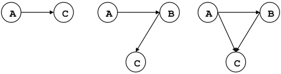
Figure 1.
(From left to right) Direct vs full indirect vs partially indirect causality.
The bivariate vector autoregression of the A and C can be represented as
with the noise covariance matrix:
By introducing B in the equation system, this becomes:
with the noise covariance matrix:
The Granger causality from A to C conditional on B is:
If the causality chain between A and C is entirely dependent on B then the coefficients λ2i should be uniformly zero and, as a consequence, the variance of the terms ε1t and ε2t is identical and therefore is equal to 1. The above reasoning can be extended to systems of more than three variables where the causality is conditioned relative to combinations of multiple time series.
Given the theoretical basis for conditional Granger causality, it is conceivable that a recursive procedure for real causal connection identification can be devised, with the scope of selecting only those coefficients in the VAR that point to direct causation. As such we have employed a network search algorithm that iteratively tests for coefficient significance as explained by Reference [4].
The variable selection algorithm iterations are the following:
- (1)
- Identify for each variable of the dataset which are the individual lags and variables that Granger cause it. These are called “ancestors”.
- (2)
- After compiling the first list of “ancestors”, each one is tested for significance in a multivariate VAR by incorporating all possible combinations of two, then three, four, etc. “ancestors”. If during this testing process the coefficient significance becomes null, the candidate “ancestor” is dropped.
- (3)
- The previous procedure iterates until all possible testing is completed, leaving only the most resilient “ancestors”.
During algorithm development, variable ordering at initialization was irrelevant to the final estimation. Regardless of variable or lag shuffling, the procedure yielded the same selection results, same coefficient values. This stands to show that the principle of conditional Granger causality is consistent for linear regression.
2.1.3. Lasso VAR
As the VAR has the tendency to become over-parametrized as the number of fitted time series grows, the estimated parameters of the model have to incorporate large amounts of white noise. In theory, OLS estimators have the property of being best linear unbiased estimators under very strong assumptions, according to the Gauss-Markov theorem. The assumptions state that the expected value of the model error terms is zero, all error terms have identic finite variance and they are uncorrelated. Take for example the general case of a linear regression: where . This matrix notation can further be expanded to . The unobserved parameters βj are said to have unbiased estimators if , where , a linear combination of only observed variables. In practice, bias is always present in the estimation results due to unaccounted factors that lead to heteroskedacity of errors and correlations between error terms.
Moving forward, OLS is an optimization technique that aims to minimize a loss function, expressed as the sum of squared residuals of the estimated model with reference to the dataset:
The expected error can be decomposed into parts determined by the “quality” of the model assumptions, the variance of the data around its long term mean, and unexplained variance:
Acknowledgement of these imperfections leads to the understanding that in any estimation procedure, one has to make a tradeoff between the bias and the variance. As the model complexity increases, the bias of OLS estimators decreases. Wanting to decrease complexity, one has to accept a higher variance. In practice, this always leads to a lower in-sample goodness of fit, but better predictions out of sample. Regularization is a technique where minimization of the loss function is penalized for model complexity.
In the case of Lasso regression, the sum of the absolute values of parameters is also subject to minimization alongside the sum of squares:
Whether it is expressed in a standard form dependent on λ or in a Lagrangian form dependent on t, choosing a value for this penalty parameters determines large regression coefficients to shrink in size and thus reduce overfitting. In comparison with ridge regression, where the sum of squared coefficients is minimized, setting a finite value for the sum of absolute coefficient value determines shrinkage of some parameters to zero which is, in fact, equivalent to variable selection.
2.1.4. Genetic VAR
Genetic algorithms represent an optimization heuristic that can generate high-quality solutions by using a global search method that mimics the evolution in the real world. Just like in nature where the fittest individuals survive adverse conditions through competition and selection, genetic algorithms resort to selection, crossover and mutation to choose between possible solutions to an optimization problem. First proposed by Reference [40], genetic algorithm procedures were formalized and tested through the work of Reference [27]. Applications of genetic algorithms in the field of statistical analysis have been limited due to their large degrees of freedom that imply a high computational cost. It should be noted that the theoretical background of evolutionary methods is yet to be defined. Nonetheless, genetic algorithms have benefited from a proven record of identifying original solutions to classical problems [41,42]. With respect to regression and VAR estimation, we must mention the recent work of References [32,35].
In the GA framework, possible solutions to an optimization problem are referred to as “individuals” or “phenotypes”. Each individual is characterized by a set of parameters that form up the individuals’ genotype or a collection of chromosomes. Evolution towards an optimal solution thus becomes an iterative procedure composed of operations like initialization, selection, crossover, mutation and novelty search. At each iteration, the fitness of each surviving individual is assessed and the fitness function represents the objective function that is being optimized.
Just like evolved organisms have necessitated millions of years to perfect themselves, genetic algorithms require numerous trials on random individuals to select the fittest ones. Translating these requirements to variable estimation in the VAR coefficient matrix, an individual is identified by (lag number × n2) + n genes, representing the lagged coefficients and the constant terms, where n is the number of variables in the system. If one coefficient is insignificant, then its corresponding gene value should be zero, meaning that the gene is inactive; otherwise, the gene expression would equal the true value of the coefficient. The purpose of the genetic algorithm is to select those individuals who have a corresponding genotype ensuring the best fitness. Just like in classical VAR estimation, the fitness/objective function should be the maximum likelihood of the model. Other fitness functions like Akaike or Bayesian criteria could be employed, but in order to compare the GA methodology with other well-known procedures, consistency must be maintained with respect to the maximum likelihood objective.
Departing from the theoretical view of linear algebraic equations, the parameter search space of a VAR can also be regarded as an infinite population of candidate solutions. From this vast population, different samples can be extracted and tested for fitness in relation to a given objective function. Through selection, feature cross-over and mutation, a process of repetitive convergence can orient the search towards a good if not optimal solution for the model parameters. In the case of the VAR the principles of competitive evolution are described as follows:
Step 1: Initialization. When doing genetic programming, ensuring a high diversity of individuals is essential for unearthing original combinations. An individual is represented by a matrix of binary entries, equal in size to the VAR matrix of coefficients (number of variables × number of lags). For bitstring chromosomes, a standard method [43] of uniformly sampling the search space is to toss a fair coin, though empirically better procedures have been proposed by Reference [44] The matrix of coefficients is reshaped into a linear vector with the same number of elements in order to create the candidate genome required for subsequent operations of mutation and cross-over, as in Figure 2.
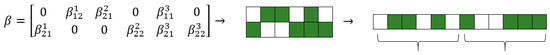
Figure 2.
Matrix of coefficients transformation to a linear vector for the candidate genome.
A zero entry represents an inactive link between a lagged variable and the explained variable specific to each VAR equation, basically a statistically insignificant coefficient. Entries equal to one refer to coefficients that will be later estimated. One requirement for the initialization step is to propose diverse individuals. The more different the proposed genotypes are, the larger the search space covered during initialization. This insight has proven most useful in the machine learning domain where new architectures for problem solving are tedious and hard to conceive [45].
The random generation of individuals can be very costly in terms of computational effort. Canonical genetic algorithms that perform complete random initialization of the population have been shown to never be able to reach a global optimum without the preservation of the best individual over generations [46]. One cause of this lies in the symmetry of the search space, where quality solutions are recombined with their complementary counterparts, resulting in random drift [47]. Moreover, to find a global solution it is necessary that the initial population set contains an individual close to the global optimum which increases time complexity, in contradiction with the optimization philosophy of quick convergence. As an example let us consider the sum of all combinations of n taken k, where n is the product (number of model variables × number of lags). According to the binomial theorem: . Therefore, the time required to go through all possible coefficient combinations grows exponentially with the number of variables and lags as shown in Table 1. One possible solution to overcome combinatorial randomness is the application of niching methods for the identification of local optima in the initial solution population [48].

Table 1.
Number of possible models to generate for different levels of complexity.
In order to better guide the inception process towards the zones of potential global optimum, the initial population is inseminated with the results of the simplified, conditional Granger and Lasso VAR. These three individuals will ensure that potentially beneficial genes are identified from the start and if so, are guaranteed to survive overall generation. This is our original approach that not only reduces computation time but as proved in the sections to follow, ensures a good model identification. By having incorporated in its initial genome a set of very fit individuals the VAR estimation algorithm does not stray towards potentially deceiving local optimum.
Step 2: Selection. Having an initial candidate population, the algorithm continues by selecting a small percentage of the fittest individuals. The fitness function takes in the binary coefficient matrix and estimates the VAR only for the non-zero parameters. The output is the matrix of estimators, together with its corresponding log-likelihood. As recommended in the literature a batch of random individuals is also selected, regardless of their fitness [49,50]. Despite being counterintuitive, experience in genetic algorithm optimization has proven that some gene combinations must survive the selection process as their utility might become relevant after a few generations [49].
One of the advantages of genetic algorithms is that the fitness function can take any form. If for OLS the mean squared error is chosen, or the likelihood function for MLE, we chose to minimize the information criteria. To be precise, the fitness function was the product of the Akaike information criterion [15] and the Bayesian information criterion [16]. Such a choice was motivated by the actual purpose of the research, that of extracting structural relations from the VAR matrix of coefficients by doing variable selection. Both of the information criteria try to strike a balance between the in-sample goodness of fit and the number of parameters used in the estimation. Denoting the value of the likelihood function with L, with n the number of observations and with k the total number of parameters, the formulae for the two information criteria are:
Step 3: Cross-over. Individuals that survived the first generations have their genotypes combined to a certain degree expressed by a percentage at choice. Similar to the natural laws of evolution, the purpose of selection is cross-over and passing of the strongest genes to off-springs. As the number of combinations can become very large even for a small batch of individuals, it is recommended that the cross-over be done between genotypes with a lower degree of similarity, as shown in Figure 3 [51].
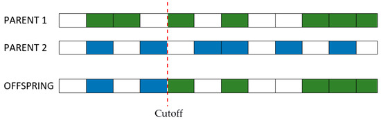
Figure 3.
Cross-over for genotypes.
Step 4: Mutation. The process of continuous selection and crossover may lead to a convergence of the optimization algorithm to local optima. It is then necessary to introduce random mutations to each generation so as to keep open other search paths that might have been missed during initialization. Just like in cross-over, a degree of mutation is chosen beforehand by the user. Precautions must be taken when setting the percentage of genes that can suffer mutations at each generation. A large coefficient can lead the optimization to becoming basically a random search. On the other hand, a small mutation degree can limit the search possibilities and not lead to a globally optimal solution.
Step 5: Fitness improvement. Iterate through steps 3 and 4 (cross-over and mutation) until the average fitness of each generation cannot be improved. The entire process can be summarized by the diagram in Figure 4.
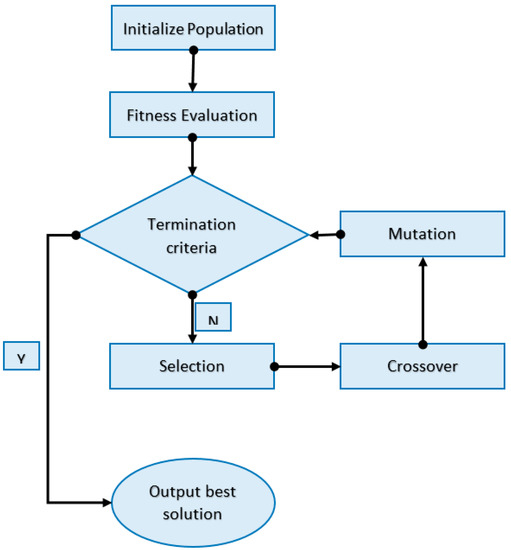
Figure 4.
Genetic algorithm procedure flow.
2.2. Performance Assessment Criteria
Any statistical estimation procedure can present different degrees of performance in-sample or out-of-sample. A higher number of estimators leads to better goodness-of-fit in-sample model but yields poor forecasting performance. An optimal model would be characterized by a parsimonious structure, a good fit on the calibration data and low error on the test data. For these reasons, the GA VAR estimation procedure was assessed through multiple criteria, as shown in Table 2.
Table 2.
Performance criteria used in simulation testing.
2.2.1. Performance Assessment of Competing Algorithms through Simulation
One of the main benefits and also the goals of variable selection in VAR estimation is the increase in model parsimony. As such, the design of the Monte Carlo simulation for testing the efficiency of the evolutionary VAR versus conditional Granger VAR, unrestricted VAR or lasso VAR, focused on expanding the data complexity on two dimensions: number of variables and number of lags. The evident expectation would be that with every step increase in the size of the matrix coefficient, the model forecast power will become diffuse, spreading equally amongst variables and lags.
Given the fact that solving for a VAR model through numerical optimization has a computational complexity of O (l × n2) for l lags and n variables, the simulations were capped at a maximum thirty variables and eight lags. Usually, VAR modeling is limited size if short or long run restrictions are not imposed on the coefficient matrix and on the covariance matrix. Moving beyond a large number of variables generates bias risk in OLS or maximum likelihood estimations.
Simulating such large VAR systems requires that the data generated remain wide-sense stationary, meaning that the mean and variance of each series are constant in time. This stability condition is equivalent to ensuring that the VARs reverse characteristic polynomial has no roots in or on the complex unit circle, which is equivalent to ensuring that in the limit the simulated processes do not reach infinity or do not converge to zero [9].
In terms of simulation parameters, we chose to test for all combinations of two to 14 variables and one to six lags. Model complexity was increased steadily in both dimensions, with an expectation for all approaches to recording a reduction in accuracy with regards to the goodness of fit and forecast power, as the size of the model grew. For each combination of lags and variable number, ten synthetic datasets were generated, independent of each other in order to average out any extreme values that might occur in the generation process. A length of 80 time steps was selected, as a proxy for almost 20 years of quarterly macroeconomic data points. For each synthetic dataset a VAR was estimated through the two proposed methods and subsequent comparison criteria were computed.
2.2.2. Performance Assessment of Competing Algorithms on Empirical Data Sets
Any statistical methodology, regardless of its theoretical grounding, has to withstand the test of real data. Both in-sample goodness of fit, as well as prediction accuracy, are ultimately the purpose of devising that methodology. Model selection algorithms have been formulated primarily to push the limits of linear modeling towards ever increasing complexity. A few decades ago, the VAR paradigm was originally conceived to leave aside the subjective assumptions economists made about the phenomena under study [2]. Giving exclusive voice to the data can work as long as the noise component acquired with it does not drive total model variance over the estimation algorithms capacity of discrimination.
Our research chose two macroeconomic different data sets for testing, each with its own purpose in revealing the advantages or limitations of the current estimation method. All series that were not stationary, were subsequently rendered so by de-trending, eliminating seasonality and taking the first difference.
US dataset—a dataset of seven macroeconomic variables for the United States economy. The choice was made to employ an identical dataset with the one used by Mathworks (https://www.mathworks.com/help/econ/examples/modeling-the-united-states-economy.html) in their example of vector error-correction (VEC) estimation, for reasons of data quality and notoriety. Moreover, this dataset was inspired by the research done on DSGE modeling for the Euro Area by [53]. The data, presented in Table 3, is collected from the Federal Reserve Economic Database for the period 1957–2016 on a quarterly frequency.
Table 3.
US macroeconomic indicators (1957:Q1 (31 March 1957) through 2016:Q4 (31 December 2016)).
Euro area dataset (the EUROZONE is composed of 19 EU member states that acceded to the zone in the following order: 11 (Austria, Belgium, Finland, France, Germany, Ireland, Italy, Luxembourg, Netherlands, Portugal and Spain) 1999; Greece 2001; Slovenia (2007), Cyprus (2008), Malta (2008), Slovakia (2009), Estonia (2011), Latvia (2014) and Lithuania (2015).)—Quarterly observations for eight macroeconomic indicators in the Euro area between Q1 2005 and Q2 2017. Due to Euro area enlargement over the years, the indicators were calculated for the entire country set depending on the year of reference. We add to this database the global oil price in the form of West Texas Intermediate (WTI). Data on Euro area macroeconomic indicators originated from Eurostat, while data for oil price was collected from the Federal Reserve Economic Database. Data are presented in Table 4.
Table 4.
Euro area macroeconomic indicators (2015:Q1–2017:Q2).
2.3. Utility of Model Shrinkage and Selection in Explaining Networks
Since its inception, the VAR has been considered a tool for revealing the interdependencies in a nation’s economy. Used by central banks, international financial institutions like the International Monetary Fund or the World Bank, the VAR methodology has been perfected to the point that it is currently used for DSGE model validation [54]. Once estimated, the VAR can serve as a simulation tool for the sensitivity of the analyzed systems through the use of impulse response functions.
Given that through variable selection the matrix of autoregressive coefficients is stripped of false causation relations, one can perceive the final estimation result as a structural representation of economic interactions. In this sense, the coefficient matrix resembles an adjacency matrix characteristic to graph theory analysis, as follows: (i) Matrix indices can be assimilated to nodes; (ii) viable coefficient positions (non-zero coefficients) are edges between nodes; (iii) coefficient signs give the edge direction; (iv) coefficient values symbolize distance measures between nodes. With all these elements in place, a graphical representation of the VAR estimation results is possible, allowing for a more direct interpretation of identified causalities. Going forward, this research focuses on a graph like the representation of the coefficient matrix by employing the minimum spanning tree topology [55].
3. Results and Discussion
Under the present section, the performance of the proposed estimation algorithms is measured. Two dimensions are given to the evaluation procedure: theoretical performance under a simulation environment and empirical performance for two different real-world data sets. Despite our best efforts to design sufficiently extensive simulations so as to converge towards idealistic testing conditions, the availability of computing power has limited the Monte-Carlo experiments to no more than 14 variable models.
3.1. Simulation Performance Results
For the simulation testing, three algorithms were chosen: unrestricted VAR, conditional Granger VAR and evolutionary VAR. The first one represents the benchmark for the last two. Despite the possibility of testing more algorithms, we decided to concentrate on the two most novel and original approaches to save computing time. Given the limited number of observations (80), for some large combinations of variables and lags, the unrestricted VAR estimation failed, due to the constraint on the covariance matrix to be positive definite.
3.1.1. Number of Estimated Model Parameters
Counting the total number of parameters to estimate, where the bias terms are also included, the simulation results show a clear difference between the three approaches. With no surprise, the unrestricted VAR presents the highest number of estimated parameters, as there is no variable selection procedure involved. In second place, the evolutionary approach drives the total parameter count to about half of the benchmark scenario. A notable difference in evolutionary VAR with respect to all other methods is the choice of an objective function oriented towards the minimization of information criteria. Such an optimization principle must take into account both model likelihood as well as the total number of parameters so it is a type of multi-objective optimization.
Continuing on the path of model complexity evaluation, the conditional Granger causality VAR is by far the most penalizing with extremely low parameter count, even for the most demanding test. For example, at 14 variables and 6-lag VAR, there are only 15 parameters to estimate. Upon the analysis of the coefficient matrix, we have observed that most of the coefficients are clustered towards the most recent lags with the rest of the matrix converging to zero. One explanation would consist in the way the conditional Granger causality principle works; if there are any collinearities between the lagged time series involved, it immediately eliminates.
Thinking of the high number of variables and lags integrated into the most complex models, the probability is high to encounter linear combinations of two or more series that explain at high accuracy another one. What is indeed surprising is the migration to most recent lags effects. Though the selection procedure for the conditional Granger VAR unravels all time lags and treats them with equal importance, it seems that time causality takes precedence. This effect has in itself sufficient logical sense as past information is to some degree integrated into the most recent realizations due to the deterministic generation process that created all observations in the first place. The visual examination of Table 5 highlights the general tendency of every approach to demand more parameters for estimation as model complexity increases.
Table 5.
Number of estimated parameters against the number of lags and variables.
3.1.2. VAR Log Likelihood
Ordinary least-squares regression is guaranteed to offer better in-sample fit as the number of explanatory variables increases. Under the present simulation, one can observe in Table 6 how unrestricted VAR produces the highest model likelihood, with an unclear differentiation between conditional Granger and evolutionary VAR. Though this result is expectable for the unrestricted approach, having similar likelihood between conditional Granger and its genetic selection counterpart proves that the in-sample fit can also be obtained through parsimonious modeling.
Table 6.
Model likelihood by number of variables and number of lags.
3.1.3. Forecast Error
A final segment of 5% from the synthetically generated data was chosen to assess prediction error. By visual inspection of Table 7, an uninformed observer can only discriminate the precedence of the last two selection algorithms over the unrestricted VAR, but cannot synthesize a conclusion over all scenarios.
Table 7.
Model MSE by number of variables and number of lags.
By means of plotting the average MSE over all lag scenarios for conditional Granger and genetic selection, followed by reporting the difference to the unrestricted approach, one can see a slight advantage for genetic algorithms (Figure 5). Better performance on prediction for the genetic selection procedure is due to the objective of optimizing both likelihood and model complexity, whereas conditional Granger causality selection focuses first on model simplification and lastly on goodness of fit.
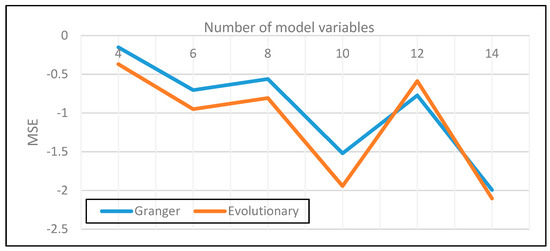
Figure 5.
Average MSE for increasing levels of complexity (difference to unrestricted VAR).
Though genetic algorithms produce slightly better predictions out of sample, it is important to mention that this type of optimization is not a universal solution for all use cases. To prove this we have conducted an additional simulation for a fixed size VAR model with eight variables and four lags and steadily increased the sample size from 50 observations up to 300 observations. Under this new simulation, depicted in Figure 6, the mean square error was indeed higher for the evolutionary approach only for small sample sizes, up to 100 observations. Beyond this threshold, all models began converging to similar prediction power. Actually, the conditional Granger and evolutionary algorithms manifest almost identical forecast errors. This proves that variable selection in VAR models should be employed only when the sample size reported to model complexity is low and the system either is under-identified or does not have sufficient observations for efficient inference.
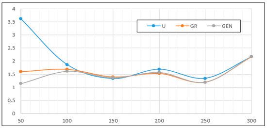
Figure 6.
Mean squared error for variable sample sizes.
3.1.4. Model Information Criteria
As a final step in the evaluation, information criteria isolate in one measurement, model efficiency. If a researcher attempts to use a model not for forecasting but for relationship inference, then information criteria point to those configurations that best describe a process in a most simple way. Both AIC and BIC criteria find a measure for the distance between the true likelihood of the data and the fitted likelihood. Information criteria have been criticized for their underlying assumptions on parameter distribution and for the fact that they might lead to over-simplified models [56]. As true as this is, any other estimation method like OLS or MLE has to resort to a distributional assumption about the data.
As BIC constantly chooses models with fewer parameters than the AIC, but in the light of the critique about over-simplification through information criteria, we chose to use both indicators in the evaluation. To be precise the product of the two criteria was calculated for all testing scenarios. These products were later scaled, with reference to the mean of all products. Comparative results can be found in Table 8.
Table 8.
Relative AIC × BIC product.
As depicted in Table 8 and Figure 7 and Figure 8, the conditional Granger causality approach produced the most efficient model selection. This is most probably due to the extremely low number of estimated parameters that yielded likelihoods and forecast errors similar to the evolutionary approach. Under these clear results, we can conclude that conditional Granger causality is a recommendable method of model selection.
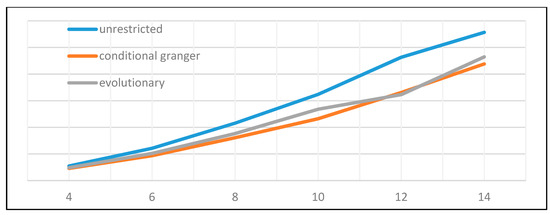
Figure 7.
Evolution of the Akaike criterion dependent on model size.
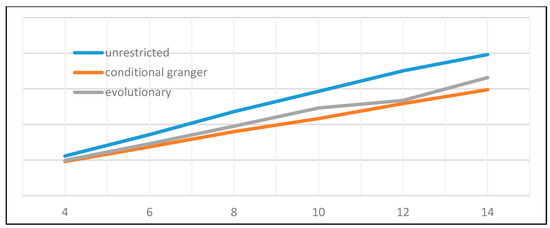
Figure 8.
Evolution of the Bayesian criterion dependent on model size.
3.2. Empirical Performance Results
3.2.1. US Economy Data Set
Table 9 presents the results of our estimations based on the US economy macroeconomic indicators datasets. Concentrating on the methodological efficiency of the genetic variable selection the most important observation focuses on the ability of the algorithm to produce the smallest mean squared error, 0.88% per observation. In the case of the forecast error, the pure GA variable selection method equals the performance of the simplified VAR algorithm. This latter method has lower likelihood but also produces a slimmer model with only 32 parameters. Moving on to the log-likelihood, the best result is represented by the unrestricted VAR, where no variable selection occurs. This is to be expected of any model that incorporates a higher and higher number estimators, which of course comes at the expense of forecast accuracy. What stands out is the ability of the GA algorithm to improve the log-likelihood of the classical unrestricted model, from 7489 to 7860, and also reduce the error from 1.02% to 0.88%. This interesting result proves that evolution through cross-over and mutation can reduce the variance of the estimators by focusing on model efficiency, a double advantageous result, from a single objective function to optimize. AIC and BIC criteria pertain only to in-sample data points but, by the elimination of unnecessary parameters, total variance and bias in the model decrease, leading to better forecasting.
Table 9.
Relative AIC × BIC product.
The lowest number of parameters, 16, is obtained, naturally, when applying the conditional Granger causality, with the objective of eliminating all indirect links between variables. A similar result is obtained for the GA modified conditional Granger causality algorithm. Moving forward to the Akaike and Bayesian information criteria, genetic algorithms produce the best results. This is most probably due to the high likelihood score that compensates for the large number of parameters employed. Overall, in the case of an empirical dataset, GA brings improvements to both coefficient estimation and model selection.
A visual interpretation of the core links in the US economy dataset identifies the great influence that personal consumption has over the overall level of the GDP and compensations of employees—see Figure 9. This observation stands out for the US economy, built on consumerism as a driving factor for growth.
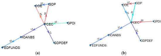
Figure 9.
Core links in the US economy dataset. (a) Granger search VAR. (b) Genetic Algortihm VAR.
3.2.2. Euro Area Dataset
Our second empirical test was conducted on the Euro area collection of macroeconomic indicators. In line from the Monte-Carlo simulations, the best performing approaches were those based on conditional Granger causality and evolutionary selection—see Table 10. A notable observation should be made for the Lasso regression algorithm: scores were good on all evaluation criteria proving that the Lasso is a balanced approach that accomplishes model selection and insures both in-sample as well as out-of-sample fit.
Table 10.
VAR estimation on the Euro area dataset.
In terms of genetic optimization design (see Figure 10), convergence reached a plateau after about ten generations with minor improvements afterwards. This shows that the initial initialization step was efficient in laying the ground for a fit future population. Our approach of insemination of competitive genes obtained from other estimation algorithms (Conditional Granger, Lasso), has reduced the search effort and diminished randomness. Under this approach, steps like initialization and selection take precedence over mutation.
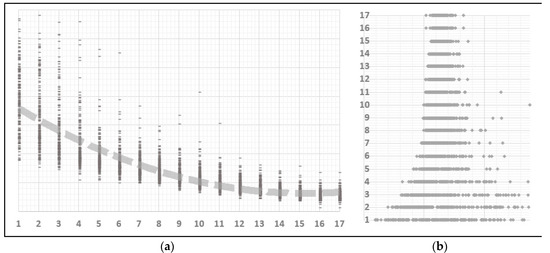
Figure 10.
Results of genetic optimization. (a) Scatter plot of solution population at each generation (b) Individual score vs. population score.
The portrayal of the evolution of the best genome of each generation highlights a stabilization of the chromosome configuration after the 14 generation—see Figure 11. Though the selection process loses power after the 10th generation as seen by the plateauing of the fitness score, focusing on the actual genome configuration, the mutation operation continues to induce change up to the 14th generation.
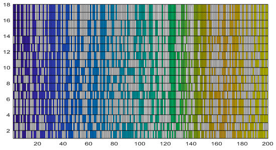
Figure 11.
Evolution of genome for the best individual at each generation.
Finalizing the Euro area analysis, a minimum spanning tree representation of the VAR coefficient matrix was rendered in graphical form under a layout that uses attractive and repulsive forces between nodes [57]. Depicting the entire coefficient matrix, the bi-directional graph shows a three-party sectioning of the underlying economic dependencies—see Figure 12. First, interest rates, oil prices and the EUR/USD exchange rate constitute a distinct group. These are also underlying assets for the most traded financial contracts on exchanges around the world. Examining the coefficients, an increase of one percentage point in interest rates triggers an increase of 0.21% in oil prices. Another chain of dependencies starts with the level of GDP and continues towards labor productivity and cost, which are in a bidirectional relationship, finishing with the consumer price index. Such a partitioning of the variables could indicate a separation of the liquid financial aspect of the economy from the real economy core. Moreover, the last chain of dependencies shows the unidirectional relationship between debt and employment, suggesting that a 1% increase in the level of debt generates a 0.64% decline in employment in the Euro area.
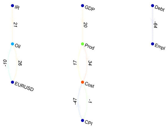
Figure 12.
Causal dependencies in the Euro area.
4. Conclusions
Model identification through variable and coefficient selection in vector autoregressions represents a continuous challenge for the scientific community. As data availability increases alongside computing power, there comes a desire to move towards much larger models, but without stepping into the sphere of subjective inference. Proposed by Reference [2] almost four decades ago, the VAR still is the preferred inference and forecasting tool in the field of macroeconomics by its virtue of giving full confidence to the data, instead of human experts.
The current research comes forward with a hybrid algorithm that mixes canonical VAR estimation methods into an evolutionary framework defined by genetic algorithms. Through extensive ample testing, both through simulation and empirical data sets, we show that genetic algorithms can partially overcome the “dimensionality curse” for those cases where data is scarce. Specifically, employing evolutionary search through the targeted generation of an initial population can lead to efficient solutions that carry in themselves the correct coefficient structure provided by other proven estimation procedures.
Whether it is a high reduction in the size of the matrix coefficient through conditional Granger causality search or a well fitted and parsimonious model through Lasso regression, the genetic selection approach can combine parts of these solutions under a user-defined objective function, for a purpose.
Departing from the current findings, we recommend that future research be oriented towards the integration of evolutionary algorithms into the field of macroeconomic forecasting. Despite their purely empirical nature, genetic algorithms can open the door to new techniques of model improvement, model fusion or even model discovery given sufficient computing power. As future research, genetic algorithms could be used in bridging the gap between linear and non-linear simultaneous equation modeling. As an example, the DSGE framework to modeling is currently based on a model being imagined by a human expert with subsequent validation by a VAR model. Genetic algorithms, through their capacity of overcoming problems with large degrees of freedom, might be a good choice for non-linear model identification in an efficient and robust manner.
Author Contributions
Conceptualization, V.G.M. and A.H.; methodology and data, V.G.M. and A.H.; software, V.G.M.; writing—original draft preparation, V.G.M. and A.H.; writing—review and editing, V.G.M. and A.H.
Funding
This research received no external funding.
Acknowledgments
We are grateful to the anonymous reviewers for their observations regarding the consistency of the methodology.
Conflicts of Interest
The authors declare no conflict of interest.
References
- Barnett, L.; Barrett, A.B.; Seth, A.K. Granger causality and transfer entropy are equivalent for Gaussian variables. Phys. Rev. Lett. 2009, 103, 238701. [Google Scholar] [CrossRef] [PubMed]
- Sims, C.A. Macroeconomics and reality. Econ. J. Econ. Soc. 1980, 48, 1–48. [Google Scholar] [CrossRef]
- Liao, W.; Mantini, D.; Zhang, Z.; Pan, Z.; Ding, J.; Gong, Q.; Yang, Y.; Chen, H. Evaluating the effectiveconnectivity of resting state networks using conditional Granger causality. Biol. Cybern. 2010, 102, 57–69. [Google Scholar] [CrossRef] [PubMed]
- Zou, C.; Ladroue, C.; Guo, S.; Feng, J. Identifying interactions in the time and frequency domains in local and global networks-A Granger Causality Approach. BMC Bioinformatics 2010, 11, 337. [Google Scholar] [CrossRef] [PubMed]
- Bellman, R. Adaptive Control Processes: A Guided Tour; Princeton University Press: Princeton, NJ, USA, 1961. [Google Scholar]
- Yamamoto, T.; Kunitomo, N. Asymptotic bias of the least squares estimator for multivariate autoregressive models. Ann. Inst. Stat. Math. 1984, 36, 419–430. [Google Scholar] [CrossRef]
- Nicholls, D.F.; Pope, A.L. Bias in the estimation of multivariate autoregressions. Aust. J. Stat. 1988, 30, 296–309. [Google Scholar] [CrossRef]
- Engsted, T.; Pedersen, T. Bias-correction in vector autoregressive models: A simulation study. Econometrics 2014, 2, 45–71. [Google Scholar] [CrossRef]
- Lütkepohl, H. New Introduction to Multiple Time Series Analysis; Springer Science & Business Media: Berlin, Germany, 2005. [Google Scholar]
- Blanchard, O.J.; Diamond, P.; Hall, R.E.; Murphy, K. The cyclical behavior of the gross flows of US workers. Brook. Pap. Econ. Act. 1990, 1990, 85–155. [Google Scholar] [CrossRef]
- Faust, J. The robustness of identified VAR conclusions about money. Carnegie Rochester Conf. Ser. Public Policy 1998, 49, 207–244. [Google Scholar] [CrossRef]
- Doan, T.; Litterman, R.; Sims, C. Forecasting and conditional projection using realistic prior distributions. Econom. Rev. 1984, 3, 1–100. [Google Scholar] [CrossRef]
- Litterman, R.B. Techniques of Forecasting Using Vector Autoregressions; Working Paper 115; Federal Reserve Bank of Minneapolis: Minneapolis, MN, USA, 1979. [Google Scholar]
- Todd, R.M. Improving economic forecasting with Bayesian vector autoregression. Model. Econ. Ser. 1990, 8, 214–234. [Google Scholar]
- Akaike, H. A new look at the statistical model identification. In Selected Papers of Hirotugu Akaike; Parzen, E., Tanabe, K., Kitagawa, G., Eds.; Springer: Basel, Switzerland, 1974; pp. 215–222. [Google Scholar]
- Schwarz, G. Estimating the dimension of a model. Ann. Stat. 1978, 6, 461–464. [Google Scholar] [CrossRef]
- Shao, J. An asymptotic theory for linear model selection. Stat. Sin. 1997, 221–242. [Google Scholar]
- Nishii, R. Asymptotic properties of criteria for selection of variables in multiple regression. Ann. Stat. 1984, 12, 758–765. [Google Scholar] [CrossRef]
- Yang, Y. Can the strengths of AIC and BIC be shared? A conflict between model indentification and regression estimation. Biometrika 2005, 92, 937–950. [Google Scholar] [CrossRef]
- Yang, Y. Regression with multiple candidate models: Selecting or mixing? Stat. Sin. 2003, 783–809. [Google Scholar]
- Hoerl, A.E.; Kennard, R.W. Ridge regression: Biased estimation for nonorthogonal problems. Technometrics 1970, 12, 55–67. [Google Scholar] [CrossRef]
- Tibshirani, R. Regression shrinkage and selection via the lasso. J. R. Stat. Soc. Ser. B Methodol. 1996, 58, 267–288. [Google Scholar] [CrossRef]
- Tibshirani, R. Regression shrinkage and selection via the lasso: A retrospective. J. R. Stat. Soc. Ser. B Stat. Methodol. 2011, 73, 273–282. [Google Scholar] [CrossRef]
- Geweke, J.F. Measures of conditional linear dependence and feedback between time series. J. Am. Stat. Assoc. 1984, 79, 907–915. [Google Scholar] [CrossRef]
- Ding, M.; Chen, Y.; Bressler, S.L. 17 Granger causality: Basic theory and application to neuroscience. Handb. Time Ser. Anal. Recent Theor. Dev. Appl. 2006, 437. [Google Scholar]
- Anghel, L.C.; Marica, V.G. Understanding Emerging and Frontier Capital Markets Dynamics through Network Theory. In Proceedings of the 5th International Academic Conference on Strategica, Bucharest, Romania, 10–11 October 2019. [Google Scholar]
- Goldberg, D.E.; Holland, J.H. Genetic algorithms and machine learning. Mach. Learn. 1988, 3, 95–99. [Google Scholar] [CrossRef]
- Leardi, R.; Gonzalez, A.L. Genetic algorithms applied to feature selection in PLS regression: How and when to use them. Chemom. Intell. Lab. Syst. 1998, 41, 195–207. [Google Scholar] [CrossRef]
- Kubiny, H. Variable selection in QSAR studies. I. An evolutionary algorithm. Quant. Struct. Act. Relatsh. 1994, 13, 285–294. [Google Scholar] [CrossRef]
- Broadhurst, D.; Goodacre, R.; Jones, A.; Rowland, J.J.; Kell, D.B. Genetic algorithms as a method for variable selection in multiple linear regression and partial least squares regression, with applications to pyrolysis mass spectrometry. Anal. Chim. Acta 1997, 348, 71–86. [Google Scholar] [CrossRef]
- Gaetan, C. Subset ARMA model identification using genetic algorithms. J. Time Ser. Anal. 2000, 21, 559–570. [Google Scholar] [CrossRef]
- Ong, C.-S.; Huang, J.-J.; Tzeng, G.-H. Model identification of ARIMA family using genetic algorithms. Appl. Math. Comput. 2005, 164, 885–912. [Google Scholar] [CrossRef]
- Chatterjee, S.; Laudato, M.; Lynch, L.A. Genetic algorithms and their statistical applications: An introduction. Comput. Stat. Data Anal. 1996, 22, 633–651. [Google Scholar] [CrossRef]
- Ursu, E.; Turkman, K.F. Periodic autoregressive model identification using genetic algorithms. J. Time Ser. Anal. 2012, 33, 398–405. [Google Scholar] [CrossRef]
- Howe, A.; Bozdogan, H. Predictive subset VAR modeling using the genetic algorithm and information complexity. Eur. J. Pure Appl. Math. 2010, 3, 382–405. [Google Scholar]
- Mirmirani, S.; Cheng Li, H. A comparison of VAR and neural networks with genetic algorithm in forecasting price of oil. In Applications of Artificial Intelligence in Finance and Economics; Binner, J.M., Kendall, G., Chen, S.H., Eds.; Emerald Group Publishing Limited: Bingley, UK, 2004; pp. 203–223. [Google Scholar]
- Geweke, J. Measurement of linear dependence and feedback between multiple time series. J. Am. Stat. Assoc. 1982, 77, 304–313. [Google Scholar] [CrossRef]
- Bressler, S.L.; Seth, A.K. Wiener–Granger causality: A well established methodology. Neuroimage 2011, 58, 323–329. [Google Scholar] [CrossRef]
- Schreiber, T. Measuring information transfer. Phys. Rev. Lett. 2000, 85, 461. [Google Scholar] [CrossRef] [PubMed]
- Fraser, A.; Burnell, D. Computer Models in Genetics; McGraw-Hill: New York, NY, USA, 1970. [Google Scholar]
- Khuda Bux, N.; Lu, M.; Wang, J.; Hussain, S.; Aljeroudi, Y. Efficient association rules hiding using genetic algorithms. Symmetry 2018, 10, 576. [Google Scholar] [CrossRef]
- Dreżewski, R.; Doroz, K. An agent-based co-evolutionary multi-objective algorithm for portfolio optimization. Symmetry 2017, 9, 168. [Google Scholar] [CrossRef]
- Bandrauk, A.D.; Delfour, M.C.; Le Bris, C. Quantum Control: Mathematical and Numerical Challenges: Mathematical and Numerical Challenges, CRM Workshop, 6–11 October 2002, Montréal, Canada; American Mathematical Soc.: Providence, RI, USA, 2003; Volume 33. [Google Scholar]
- Kallel, L.; Schoenauer, M. Alternative Random Initialization in Genetic Algorithms. In Proceedings of the 7th International Conference on Genetic Algorithms (ICGA 1997), Michigan State University, East Lansing, MI, USA, 19–23 July 1997; pp. 268–275. [Google Scholar]
- Lehman, J.; Stanley, K.O. Abandoning objectives: Evolution through the search for novelty alone. Evol. Comput. 2011, 19, 189–223. [Google Scholar] [CrossRef]
- Rudolph, G. Convergence analysis of canonical genetic algorithms. IEEE Trans. Neural Netw. 1994, 5, 96–101. [Google Scholar] [CrossRef]
- Pelikan, M.; Goldberg, D.E. Genetic Algorithms, Clustering, and the Breaking of Symmetry. In Proceedings of the International Conference on Parallel Problem Solving from Nature, (PPSN 2000), Paris, France, 18–20 September 2000; Springer: Basel, Switzerland, 2000; pp. 385–394. [Google Scholar]
- Mahfoud, S.W. Niching Methods for Genetic Algorithms. Ph.D. Thesis, University of Illinois at Urbana-Champaign, Champaign, IL, USA, 1995. [Google Scholar]
- Lehman, J.; Stanley, K.O. Evolving a Diversity of Virtual Creatures through Novelty Search and Local Competition. In Proceedings of the 13th Annual Conference on Genetic and Evolutionary Computation, Dublin, Ireland, 12–16 July 2011; ACM: Ney York, NY, USA, 2011; pp. 211–218. [Google Scholar]
- Valls, V.; Ballestin, F.; Quintanilla, S. A hybrid genetic algorithm for the resource-constrained project scheduling problem. Eur. J. Oper. Res. 2008, 185, 495–508. [Google Scholar] [CrossRef]
- Mouret, J.-B. Novelty-based multiobjectivization. In New Horizons in Evolutionary Robotics; Doncieux, S., Bredeche, N., Mouret, J.P., Eds.; Springer: Basel, Switzerland, 2011; pp. 139–154. [Google Scholar]
- Johansen, S. Likelihood-Based Inference in Cointegrated Vector Autoregressive Models; Oxford University Press on Demand: Oxford, UK, 1995. [Google Scholar]
- Smets, F.; Wouters, R. An estimated dynamic stochastic general equilibrium model of the euro area. J. Eur. Econ. Assoc. 2003, 1, 1123–1175. [Google Scholar] [CrossRef]
- Giacomini, R. The relationship between DSGE and VAR models. In VAR Models in Macroeconomics—New Developments and Applications: Essays in Honor of Christopher A. Sims; Fomby, T.B., Murphy, A., Kilian, L., Eds.; Emerald Group Publishing Limited: Bingley, UK, 2013; pp. 1–25. [Google Scholar]
- Dijkstra, E.W. A note on two problems in connexion with graphs. Numer. Math. 1959, 1, 269–271. [Google Scholar] [CrossRef]
- Weakliem, D.L. A critique of the Bayesian information criterion for model selection. Sociol. Methods Res. 1999, 27, 359–397. [Google Scholar] [CrossRef]
- Fruchterman, T.M.; Reingold, E.M. Graph drawing by force-directed placement. Softw. Pract. Exp. 1991, 21, 1129–1164. [Google Scholar] [CrossRef]
© 2019 by the authors. Licensee MDPI, Basel, Switzerland. This article is an open access article distributed under the terms and conditions of the Creative Commons Attribution (CC BY) license (http://creativecommons.org/licenses/by/4.0/).