Individual-Specific Classification of Mental Workload Levels Via an Ensemble Heterogeneous Extreme Learning Machine for EEG Modeling

Abstract

In a human–machine cooperation system, assessing the mental workload (MW) of the human operator is quite crucial to maintaining safe operation conditions. Among various MW indicators, electroencephalography (EEG) signals are particularly attractive because of their high temporal resolution and sensitivity to the occupation of working memory. However, the individual difference of the EEG feature distribution may impair the machine-learning based MW classifier. In this paper, we employed a fast-training neural network, extreme learning machine (ELM), as the basis to build an individual-specific classifier ensemble to recognize binary MW. To improve the diversity of the classification committee, heterogeneous member classifiers were adopted by fusing multiple ELMs and Bayesian models. Specifically, a deep network structure was applied in each weak model aiming at finding informative EEG feature representations. The structure of hyper-parameters of the proposed heterogeneous ensemble ELM (HE-ELM) was then identified and then its performance was compared against several competitive MW classifiers. We found that the HE-ELM model was superior for improving the individual-specific accuracy of MW assessments.

1. Introduction

In various human–machine (HM) cooperation systems—such as driving systems, brain–computer interface (BCI) systems, nuclear power plants and air traffic control [1]—it is difficult for human operators to maintain effective functional states when performing longtime duration tasks with a high complexity level. The reason behind this is that human cognitive capacity is affected and limited by multidimensional psychophysiological factors. It thus leads to unstable task performance compared to machine agents. One of the most important aspects of operator functional states (OFSs) is termed as mental workload (MW). It can be generally defined as the remaining cognitive resource or capacity of working memories under transient task demand [2].

Understanding the MW functionality can facilitate human-centered automation systems that both improve the safety and satisfaction level of the HM interaction. Aricò et al. [3] mentioned that the scope of the brain computer interfacing (BCI) system has been extended over the past decade and its functionality involves the monitoring of cognitive workload and emotional states that are identified by the user’s spontaneous brain activity. Since the human executive capability is closely linked to temporal stress, operators could fail to make a prompt response for handling emergency events under their limited working memory. To prevent the resulting safety-critical errors, it is significant to discern MW levels, with the aim of predicting the temporal trend of human performance degradation. The operator MW involved in the human–machine system can be assessed indirectly through task performance, subjective assessment, and psychophysiological measurements [4,5,6]. Among these measurements, the subjective assessment has the limitation of low time resolution since it requires the operator to report their cognitive load. The task performance indicator alone is not satisfactory due to the fact that the MW may increase with the performance indicator unchanged. The psychophysiological measurement is considered to be superior because it can be objectively and continuously acquired [4].

In the past few years, neural signal analysis techniques on various physiological biomarkers, e.g., electroencephalogram (EEG), electrooculogram (EOG), and electrocardiogram (ECG), have been used to provide the basis of quantitative, real-time evaluation of MW variation [7,8]. In particular, EEG features were implemented with portable recording devices as useful MW indicators in well-documented works. Since the EEG reflects the functionality and cognitive states of the central nervous system, it has been widely used to evaluate the MW. The reported works showed that the MW can be accurately predicted by analyzing changes in EEG power spectral density (PSD) [9,10]. The input data used in the experiment is a matrix. The number of rows in the matrix represents the number of samples, and the number of columns in the matrix represents the number of EEG power spectral density features. The specific element values in the matrix represent the values of the features of the current sample.

Aricò et al. [11] validated this passive BCI system in evaluating operator workload of high-altitude air traffic control missions with varying difficulty. This work also investigated the possibility of assessing operator MW in real time. The work of many other researchers on MW assessment is as follows. Moon proposed an ECG/EEG-data-driven fuzzy system to quantify MW [12]. Obinata et al. [13] employed vestibule-ocular reflex (VOR) features from EOG as MW indicators. Their results show that the VOR measure is effective and sensitive to the transient variation of the cognitive capability. Ryu and Myung [14] presented a comprehensive framework combining multimodal measurements of EEG, ECG, and EOG to classify MW when the operator was engaged in a dual task. It was reported that such integrated method outperformed the case with the single modality. Dimitrakopoulos et al. [15] proposed an EEG based classification framework, where multi-band functional connectivity is used to predict within-task and cross-task MW levels. Ayaz et al. [16] proposed the MW recognition system using functional near-infrared spectroscopy (fNIRS). The results showed that the fINRS features have the capability to monitor hemodynamic changes associated with the operator cognitive stress. The fNIRS can evaluate MW by indirectly judging oxygen consumption by changes in oxygen content in blood vessels.

Due to the uncertainty, complexity, and multidimensionality of EEG features, machine learning based modeling approaches are attractive for classifying the extracted neurophysiological markers into multiple MW levels. The state-of-the-art MW classifiers include neural network [17], fuzzy system [12], random forest, stacked denoising autoencoder (SDAE), and support vector machine (SVM) [18]. In addition, Mazaeva et al. [19] proposed a hybrid self-organizing feature mapping network to predict the level of MW. They also adopted a shallow neural network to establish the link between EEG features and the MW states. The reported results showed that the testing classification accuracy was achieved to 89%. Javier et al. [20] adopted a dendrite morphological neural network (DMNN) for the recognition of mental tasks based on EEG signals, where the classification accuracy of motor execution was achieved to 80%. In [12], the fuzzy inference system was reported to be superior to the classical linear modeling method for discriminating MW classes. Yin and Zhang proposed an EEG based adaptive SDAE model for tackling a cross-session MW classification problem [21]. Zhao et al. [22] employed an EEG-based SVM to detect the variation of MW when operators were performing different cognitive tasks. Both of the physiological and behavioral measurements were used in their work to assess MW into four categories. The target class label was determined via the degree of task difficulty with the overall classification accuracy of 95% achieved.

In newly reported works, extreme learning machine (ELM) has been validated in multiple EEG classification tasks. The ELM was originally developed based on single-hidden-layer feedforward neural networks (SLFNs) [23] with random input weights [24]. In medium size classification applications [25], the training speed of the ELM classifier was significantly higher than the SVM using a radial basis kernel function [26] and the back-propagation (BP) neural networks. In large complex real-world datasets [27], the competitive classification accuracy of ELM benefits from random feature mapping, where the gradient based optimization methods are unnecessary [28]. ELM classifier was used in recognizing motor imagery tasks via EEG signals with acceptable performance and low computational cost [29,30,31]. In [32], EEG signals combined with ELM have been implemented for operator vigilance estimation. In these HM interaction systems, the ELM model was trained by the extracted EEG features and implemented in a real-time EEG analysis environment for medical assistants.

The goal of the present study is to design an individual-specific MW classifier since the data distribution of the EEG features may vary across multiple subjects. That is, we need to find a personalized classifier architecture for each task operator. To this end, the ensemble learning principle is employed to achieve multiple classifier committees on different subjects. In particular, a large amount of training EEG instances are required for building the member classifier in such a committee while ELM is more suitable for such implementation due to its high training speed than conventional ANN and SVM based methods. Despite its high training speed, the ELM algorithm has a number of problems with the application. The output weight of the ELM model is fixed and may not be suitable for EEG data of all subjects. Therefore, we construct an abstraction layer in each weak ELM to find the intermediate EEG feature representations to improve the interclass discrimination capability. On the basis of the ELM ensemble and the deep feature mapping, we proposed a new approach for personal MW recognition called heterogeneous ensemble extreme learning machine (HE-ELM), where the member classifiers possess inherent heterogeneous structures aimed at improving the diversity of the classification committee. The main novelty of the HE-ELM algorithm is the integration of multiple heterogeneous strong classifiers with adaptive structures and hyper-parameters. This characteristic facilitates designing personalized workload classifiers for different individuals. In classical schemes, weak classifiers are generally consistent, and the final classification committee may not possess the flexibility to learn individual-specific information of EEG feature distributions. The HE-ELM is also helpful in improving the diversity between weak classifiers and reducing the upper boundary of the generalization capability. The HE-ELM with its heterogeneous nature facilitating the introduction of other classifiers, is a great difference to deep ELMs.

The organization of the paper is as follows. In Section 2.1 and Section 2.2, the EEG database for classifier validation is described. Section 2.3, Section 2.4 and Section 2.5 reviews the classical ELM algorithm and presents the new HE-ELM method. The detailed MW classification results are shown in Section 3. In Section 4, we discuss the derived results. Finally, the present study is concluded in Section 5.

2. Materials and Methods

2.1. Experimental Tasks and Subjects

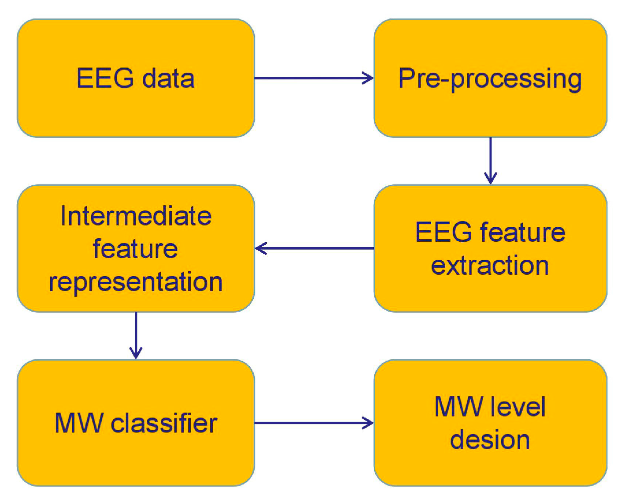
The EEG database used for testing the proposed algorithm was built in our previous work [33]. The framework of MW level assessment is described in Figure 1. We simulated the HM collaboration environment via a software platform termed as automation-enhanced cabin air management systems (ACAMS) [7,34,35]. This experiment used a simplified version of automation-enhanced cabin air management systems (ACAMS) and consisted of loading and unloading phases. ACAMS consisted of four subsystems: Air pressure, temperature, carbon dioxide concentration and oxygen concentration. The function of ACAMS is to observe and control the air quality in the closed space of the spacecraft. This software platform is used to simulate a safety-critical human–machine collaboration environment. Subjects need to concentrate on the operation because the trajectory can easily exceed the target range. Under the ACAMS, the ongoing physiological data of operators corresponding to different task complexities were acquired and used for modeling their transient MW level. The operation of the tasks was related to the maintenance of the air quality in a virtual spacecraft via human-computer interaction.

Figure 1. The framework of assessing MW levels.

Operators were required to manually monitor and maintain four variables (O₂ concentration, air pressure, CO₂ concentration, temperature) to their respective ranges according to given instructions. That is, when any of the subsystems’ program runs incorrectly, operators manually control the task until the systems error is fixed. Simultaneously, the current EEG signals were recorded. The complexity for performing control tasks is measured by the number of manually controlled subsystems (NOS). According to different value of NOS, the complexity and demand of the manual control tasks is gradually changing, which can induce a variation of the MW.

Eight male participants (22–24 years) were engaged and coded by S1, S2, S3, S4, S5, S6, S7, and S8. All participants were volunteer graduate students from the East China University of Science and Technology. All participants have been trained in ACAMS operations for more than 10 h before the start of the formal experiment. As can be seen from our previous work [36], the average task performance was analyzed and its mean value of all subjects in the first control condition was not significantly varied compared with the last control condition (i.e., from 0.957 to 0.936). Moreover, all subjects cannot perfectly operate the ACAMS of high task complexity in both sessions (with average task performance of 0.783). Since the task demands in the high difficulty conditions were the same across two sessions, the habituation effect of subjects was properly controlled. The reason behind this is that each participant was trained for more than 10 h before the formal experiment and their task performance properly converged.

To rule out the effects of the circadian rhythm, each subject conducted the experiment from 2:00 p.m. to 5:00 p.m. for different sessions. The participants were required to perform two identical sessions of experiments. Each session consisted of eight control task load conditions. After the starting 5-min baseline condition under NOS with the value of 0, there were six 15-min conditions followed by the last 5-min baseline condition again. The duration of each session was 100 min (100 = 6 × 15 + 2 × 5). The operator’s cognitive demand for manual tasks were gradually increased and then reduced within 100 min in one session. We selected the EEG data from six, 15-min conditions in each session. A total of 16 (2 × 8) physiological datasets were built. Under conditions #1, #2, #3, #4, #5, and #6, the participants needed to manually operate ACAMS under NOS with the value of 2, 3, 4, 4, 3, and 2. The subjective rating analysis was omitted and can be found in our previous work [33].

2.2. EEG Feature Extraction

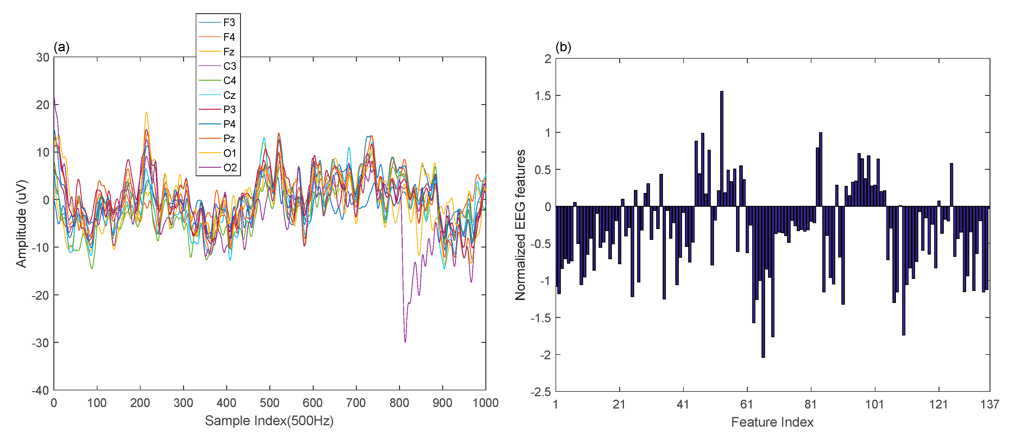
The raw EEG signals and the extracted EEG features are depicted in Figure 2. The EEG data were measured via the 10–20 international electrode system on 11 positions of the scalp (i.e., F3, F4, Fz, C3, C4, Cz, P3, P4, Pz, O1, and O2) at the frequency of 500 Hz. Frontal theta power and the parietal alpha were used for MW variation detection. In addition, we also noticed that the EEG power of the alpha frequency band in the central scalp region degreases along with the increase of the MW according to [37,38,39]. In [40], the EEG power of the occipital channels was shown to be related to the stress and fatigue. Therefore, in order to improve the diversity of the possible EEG features that were salient to workload variation, the central and occipital electrodes were also employed in the experiment. To cope with the electromyography (EMG) noise, the independent component analysis (ICA) was employed to filter the raw EEG data. The independent component associated with the muscular activity was identified by careful visual inspection and was eliminated before extracting EEG features. Moreover, the ACAMS operations were not heavily depended on the sensory motor functionality of the cortex. If such noise exists, the possible EEG clues could be allocated with small weight values since the supervised machine learning algorithm only adopted MW levels as target classes. Therefore, the irrelevant EEG indicators can be well controlled.

Figure 2. The raw EEG data in (a) a 2-s segment of 11 channels and (b) the corresponding 137 EEG features.

The preprocessing steps of the acquired EEG signals are shown as follows:

(1)

All EEG signals were filtered through a three-order low-pass IIR filter with a cutoff frequency of 40 Hz. The related works [41,42,43] indicated that removing EOG artifacts can improve the EEG classification rate, the blink artifacts in EEG signals were eliminated by the coherence method in this study. According to our previous work [33], the blink artifact was removed by the following equation

$$d(t)=\widehat{d}(t)-C\cdot {\widehat{d}}^O(t)$$

(1)

In the equation, the EEG signal and the synchronized EOG signal at the time instant $t$ are denoted by $\widehat{d}(t)$ and ${\widehat{d}}^O(t)$, respectively. The transfer coefficient $C$ is defined by

$$C=\frac{\frac{1}{N}{\displaystyle \sum _{t=1}^N\left[\left(\widehat{d}(t)-\overline{\widehat{d}}\right)\left({\widehat{d}}^O(t)-{\overline{\widehat{d}}}^O\right)\right]}}{\frac{1}{N}{\displaystyle \sum _{t=1}^N{\left({\overline{\widehat{d}}}^O(t)-{\overline{\widehat{d}}}^O\right)}^2}}$$

(2)

where $N$ denotes the number of samples in an EEG segment, $\overline{\widehat{d}}$ and ${\overline{\widehat{d}}}^O$ are the means of EEG signal and synchronized EOG signal in a channel, respectively.

(2)

The filtered EEG was divided into 2-s segments and processed with a high-pass IIR filter (cutoff frequency of 1 Hz) to remove respiratory artifacts.

(3)

Fast Fourier transform was adopted to compute the power spectral density (PSD) features of the EEG signals. For each channel, four features were obtained by the calculated PSD within theta (4–8 Hz), alpha (8–13 Hz), beta (14–30 Hz), and gamma (31–40 Hz) frequency bands. Based on the PSD features from F3, F4, C3, C4, P3, P4, O1, and O2, we further computed sixteen power differences between the right and left hemispheres of the scalp. That is, 60 frequency domain features were extracted. Then, 77-time domain features were elicited via mean, variance, zero crossing rate, Shannon entropy, spectral entropy, kurtosis, and skewness of 11 channels. The indices and notations of 137 EEG features are shown in Table 1.

Table 1. The serial number and notations of the electroencephalography (EEG) features.

Feature Index	Feature Notations
No. 1–11	Centroid frequencies of 11 channels
No. 12–22	Log energy entropies of 11 channels
No. 23–33	Means of 11 channels
No. 34–77	Average PSDs in theta (4–8 Hz), alpha (8–13 Hz), beta (14–30 Hz) and gamma (31–40 Hz) frequency bands of 11 channels
No. 78–93	Power differences between the right and left hemispheres of the scalp
No. 94–04	Shannon entropies of 11 channels
No. 105–115	Sums of energy of 11 channels
No. 116–126	Variances of 11 channels
No. 127–137	Zero-crossing rates of 11 channels

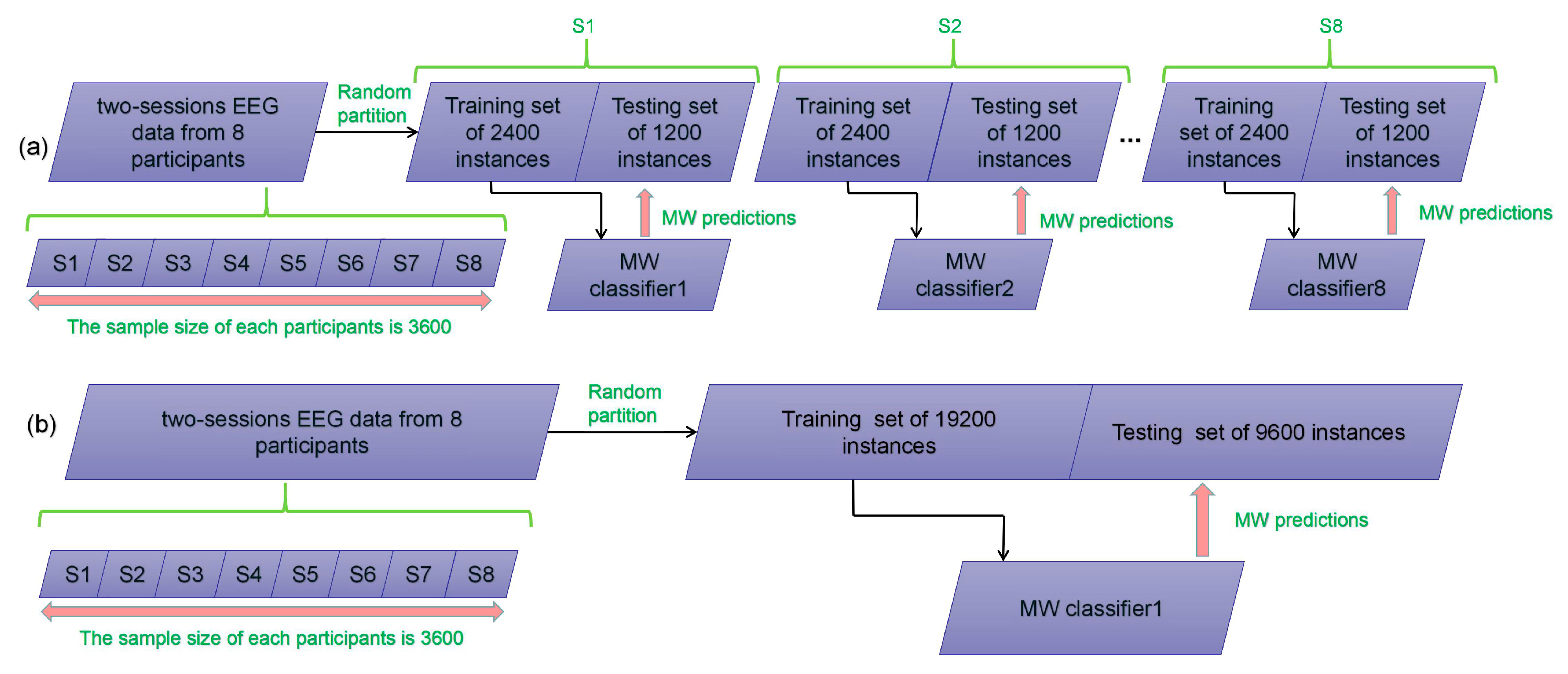
Finally, there were 8 subjects in the experiment, and each subject had two feature sets. Each feature set is a matrix of the same size. The number of rows of the matrix is 1800 for the number of data points, and the number of columns of the matrix is 137 for the number of features. That is, 28,800 data points are available in total. Each feature was normalized into the time course of zero mean and one standard deviation. The EEG vectors were assigned the MW labels of low and high classes and quantified as $\mathbf{y}=[\begin{array}{cc}1& 0\end{array}]$ and $\mathbf{y}=[\begin{array}{cc}0& 1\end{array}]$, respectively. Note that the first and the last 450 EEG instances in each feature matrix represent a low MW level and the remaining 900 points correspond to high MW levels.

2.3. Extreme Learning Machine

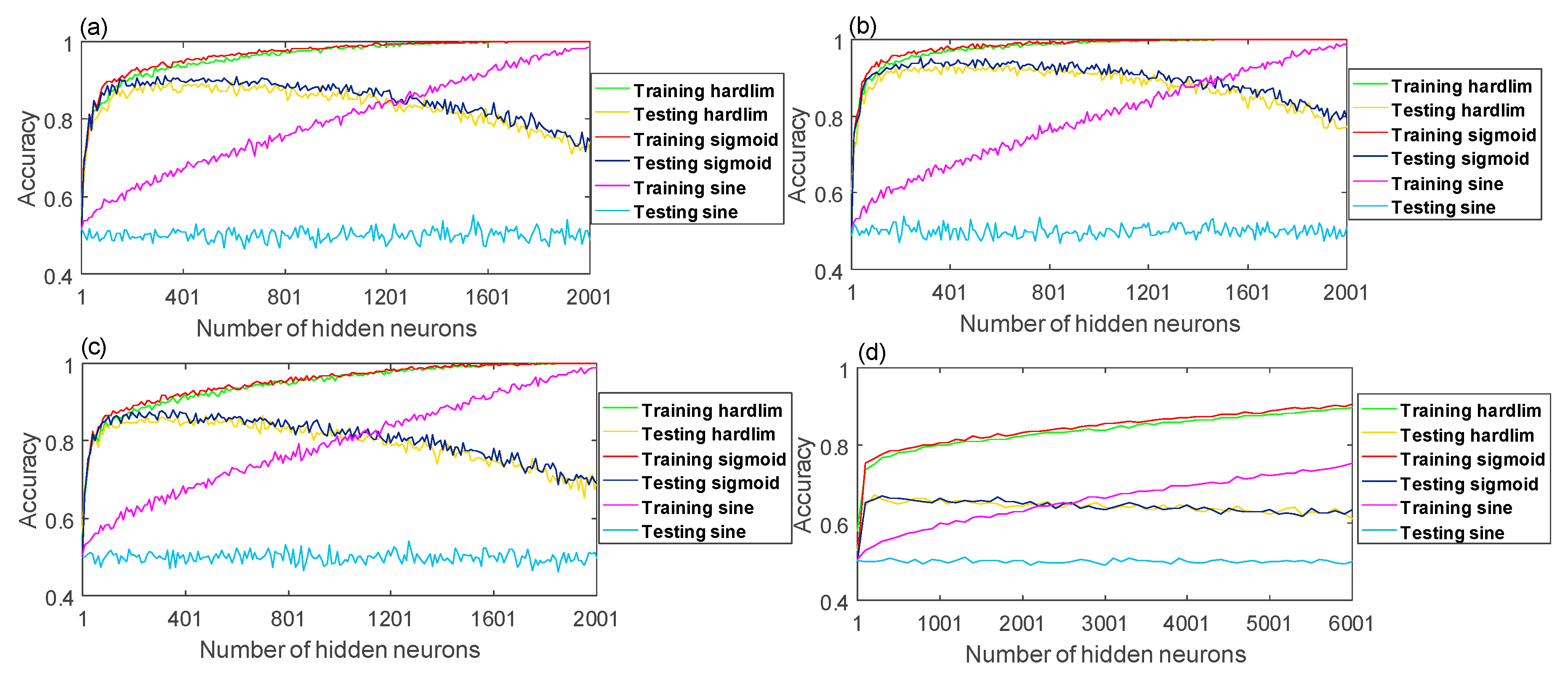
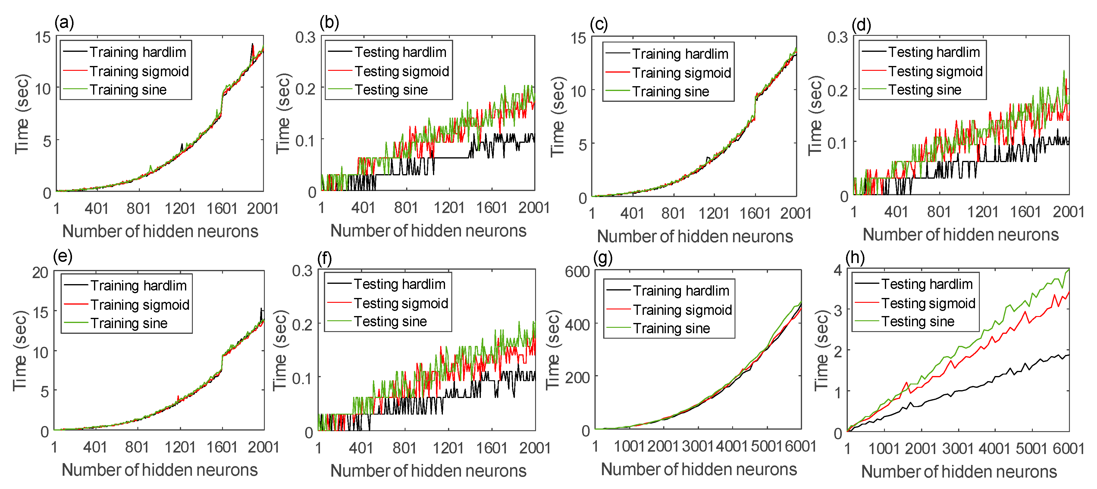
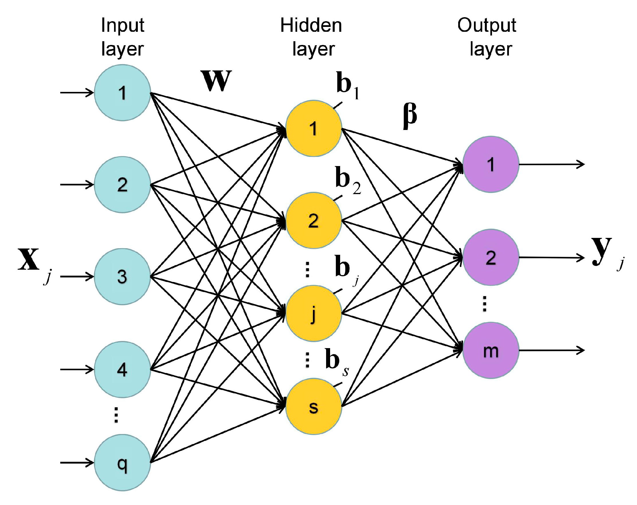
ELM is a fast-training modeling approach based on SLFN [44,45]. Figure 3 shows a typical SLFN-based ELM architecture, where ${\mathbf{x}}_i={[x_{i1},x_{i2},\dots ,x_{iq}]}^{\mathrm{T}}$ is the input sample array and the corresponding output label array is ${\mathbf{y}}_i={[y_{i1},y_{i2},\dots ,y_{im}]}^{\mathrm{T}}$. Let denote the input weights, output weights, and bias of the hidden neuron as ${\mathbf{w}}_j={[w_{j1},w_{j2},\dots ,w_{jq}]}^{\mathrm{T}}$, ${\mathsf{\beta }}_j={[{\beta }_{j1},{\beta }_{j2},\dots ,{\beta }_{jm}]}^{\mathrm{T}}$, and ${\mathbf{b}}_j$, respectively. Training a SLFN as an ELM is equivalent to minimizing the output error between the target output ${\mathbf{y}}_i$ and model output ${\widehat{\mathbf{y}}}_i$ regarding to the parameters, ${\mathsf{\beta }}_j$, ${\mathbf{b}}_j$ and ${\mathbf{w}}_j$, i.e.,

Figure 3. The architecture of a typical single-hidden-layer feedforward neural networks (SLFN) training by ELM.

$${\displaystyle \sum _{j=1}^S{\mathsf{\beta }}_j\cdot p(}{\mathbf{w}}_j\cdot {\mathbf{x}}_i+{\mathbf{b}}_j)={\widehat{\mathbf{y}}}_i,i=1,2,\dots ,\tilde{S}$$

(3)

In Equation (3), $\tilde{S}$ is the number of EEG samples, $p(\cdot )$ is the activation function. The number of the input, output and hidden neurons are defined as $q$, $m$, and $S$, respectively. The training cost function is formulated in a least squared term,

$$E={{\displaystyle \sum _{i=1}^{\tilde{S}}\left[{\displaystyle \sum _{j=1}^S{\mathsf{\beta }}_j\cdot p({\mathbf{w}}_j\cdot {\mathbf{x}}_i+{\mathbf{b}}_j)-{\mathbf{y}}_i}\right]}}^2.$$

(4)

Traditional neural network training approaches are mostly based on gradient descent optimization via BP algorithm. On the contrary, in the process of the ELM modeling the input weights and hidden layer bias are randomly determined while all output weights of hidden layer are computed via the norm minimization-based approach. To this end, it is unnecessary to tune the input weights and hidden layer bias in the training process.

Based on the input weights and bias that are randomly selected, the model fitting error in Equation (4) can be derived via a linear equation systems, $\mathbf{H}\mathsf{\beta }=\mathbf{Y}$, where $\mathbf{H}$ is the output matrix of the hidden layer. The entry of $\mathbf{H}$ is denoted as follows

$$\mathbf{H}({\mathbf{w}}_1,\dots ,{\mathbf{w}}_2,{\mathbf{b}}_1,\dots ,{\mathbf{b}}_2,{\mathbf{x}}_1,\dots ,{\mathbf{x}}_{\tilde{S}})=\left[\begin{array}{ccc}p({\mathbf{h}}_1^{(1)})& \cdots & p({\mathbf{h}}_S^{(1)})\\ ⋮& \cdots & ⋮\\ p({\mathbf{h}}_1^{(\tilde{S})})& \cdots & p({\mathbf{h}}_S^{(\tilde{S})})\end{array}\right]$$

(5)

In Equation (5), the induced local field, ${\mathbf{h}}_j^{(i)}$, is computed via the function signal below

$${\mathbf{h}}_j^{(i)}=p({\mathbf{w}}_j\cdot {\mathbf{x}}_i+{\mathbf{b}}_j),i=1,2,\dots ,\tilde{S},j=1,2,\dots ,S$$

(6)

Thus, the output weight $\mathsf{\beta }$ can be elicited by the generalized inverse matrix operation

$$\mathbf{H}\mathsf{\beta }=\mathbf{Y}\to \overline{\mathsf{\beta }}={\mathbf{H}}^{\ast }\mathbf{Y}$$

(7)

where ${\mathbf{H}}^{\ast }$ denotes the Moore-Penrose generalized inverse of matrix $\mathbf{H}$ [27]. Singular value decomposition can be implemented to compute ${\mathbf{H}}^{\ast }$. The pseudo codes of the ELM training algorithm are summarized in Table 2 [46]. In the pseudo code, the training set, activation function, the number of hidden nodes, and the output weights are defined as $\{\mathbf{X},\mathbf{Y}\}$,$p(\cdot )$,$S$ and $\mathsf{\beta }$, respectively. The remaining parameters are consistent with the above.

Table 2. Pseudo codes for training an extreme learning machine (ELM).

ELM_Train$\left(\mathbf{X},\mathbf{Y},p,S\right)$
1	Randomly assigned $\mathbf{W},\mathbf{b}$
2	for$i$ = 1 to $\tilde{S}$, $j$ = 1 to $S$
3	${\mathbf{h}}_j^{(i)}=\mathrm{p}({\mathbf{w}}_j\cdot {\mathbf{x}}_i+{\mathbf{b}}_j)$
4	Compute $\mathbf{H}$ according to Equation (5)
5	Compute the generalized inverse ${\mathbf{H}}^{\ast }$ of $\mathbf{H}$
6	$\mathsf{\beta }={\mathbf{H}}^{\ast }\mathbf{Y}$
7	return$(\mathbf{W},\mathbf{b},\mathsf{\beta })$

2.4. Adaboost Based ELM Ensemble Classifier

To improve the classification accuracy of MW on EEG datasets, we introduced the ELM classifier ensemble to find different individual personalities existing in EEG features. The framework of the ELM ensemble is designed based on the adaptive boosting algorithm (Adaboost) [47]. In the classical boosting algorithm [48], each training instance is given with an initial weight before the training procedure begins while the value of the weight is automatically adjusted during each iteration. In particular, the Adaboost algorithm adds a new classifier in each training iteration and additionally constructs several weak classifiers on the same sample pool. A strong classifier can thus be integrated via those weak classifiers.

To implement the Adaboost method into the ELM ensemble, we first initialized the weights of each training data of $N$ training instances with $w_i=1/N$, $i=1,2,\dots ,N$. That is, the initial weights of the sample are ${\mathbf{D}}_1={[{\tilde{w}}_1,{\tilde{w}}_2,\dots ,{\tilde{w}}_N]}^T$. Then, we ran $m$ ($m=1,2,\dots ,M$) iterations to select a basic classifier $G_m$ possessing the highest classification precision. The error rate of the selected classifier on the ${\mathbf{D}}_m$ is computed by

$$e_m=P[G_m({\mathbf{x}}_i)\ne {\mathbf{y}}_i]={\displaystyle \sum _{i=1}^N{\tilde{w}}_{mi}}I[G_m({\mathbf{x}}_i)\ne {\mathbf{y}}_i]$$

(8)

In Equation (8), ${\mathbf{x}}_i$ denotes the input sample array, ${\mathbf{y}}_i$ corresponds to output label array, $I(\cdot )$ represents statistics that ${\mathbf{x}}_i$ is wrongly classified. If ${\mathbf{x}}_i$ is correctly (or incorrectly) classified, $I=0$ or ($I=1$) exists. The weight of $G_m$ in the final strong classifier $G_s$ is computed by the following equation

$${\lambda }_m=\frac{1}{2}\ln \left(\frac{1-e_m}{e_m}\right)$$

(9)

According to [47], the weight distribution of the training sample is updated via

$${\mathbf{D}}_{m+1}=\frac{{\mathbf{D}}_m(i)\exp [-{\lambda }_m{\mathbf{y}}_i{G}_m({\mathbf{x}}_i)]}{2\sqrt{e_m(1-e_m)}}$$

(10)

The output of the strong classifier $G_s$ is integrated from the weak classifiers through the weight ${\lambda }_m$ as follows

$${\mathbf{y}}_s=\mathrm{sign}\left({\displaystyle \sum _{m=1}^M{\lambda }_m{G}_m(\mathbf{x})}\right)$$

(11)

In Equation (11), ${\mathbf{y}}_s$ is the final output of the classifier. The pseudo codes of the Adaboost ELM is presented in Table 3 [46], where the maximum number of iterations is $M$, the weight of each weak classifier is ${\lambda }_m$ and the output of the strong classifier is $G_s(\cdot )$. The remaining parameters are consistent with the above.

Table 3. The pseudo codes for the Adaboost ELM algorithm.

ELM_Adaboost$\left(\mathbf{X},\mathbf{Y},p(\cdot ),S,M\right)$
1	${\mathbf{D}}_1={[1/N,1/N,\dots ,1/N]}^T$
2	for$m$ = 1 to $M$
3	ELM_train $(\{\mathbf{X},\mathbf{Y}\},\mathrm{p},S)$
4	return $G_m(\cdot )$
5	Compute predictive output as $G_m(\mathbf{x})$
6	$e_m={\displaystyle \sum _{i=1}^N{\mathbf{D}}_m(i)}I[G_m({\mathbf{x}}_i)\ne {\mathbf{y}}_i]$
7	${\lambda }_m=1/2\ln [(1-e_m)/e_m]$
8	Update ${\mathbf{D}}_{m+1}$ according to Equation (9)
9	${\mathbf{y}}_s=\mathrm{sign}[{\displaystyle {\sum }_{m=1}^M{\lambda }_m{G}_m(\mathbf{x})]}$
10	return${\mathbf{y}}_s$

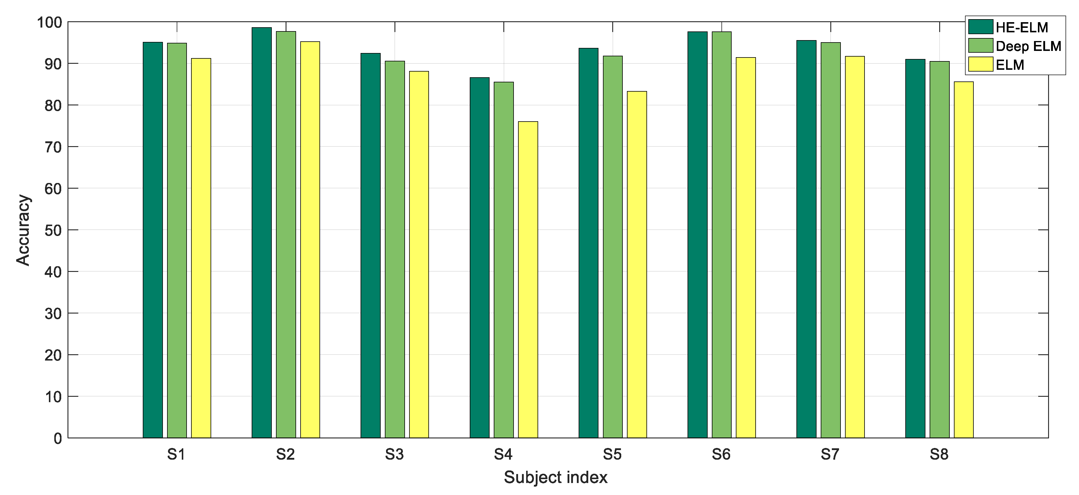
2.5. Heterogeneous Ensemble ELM

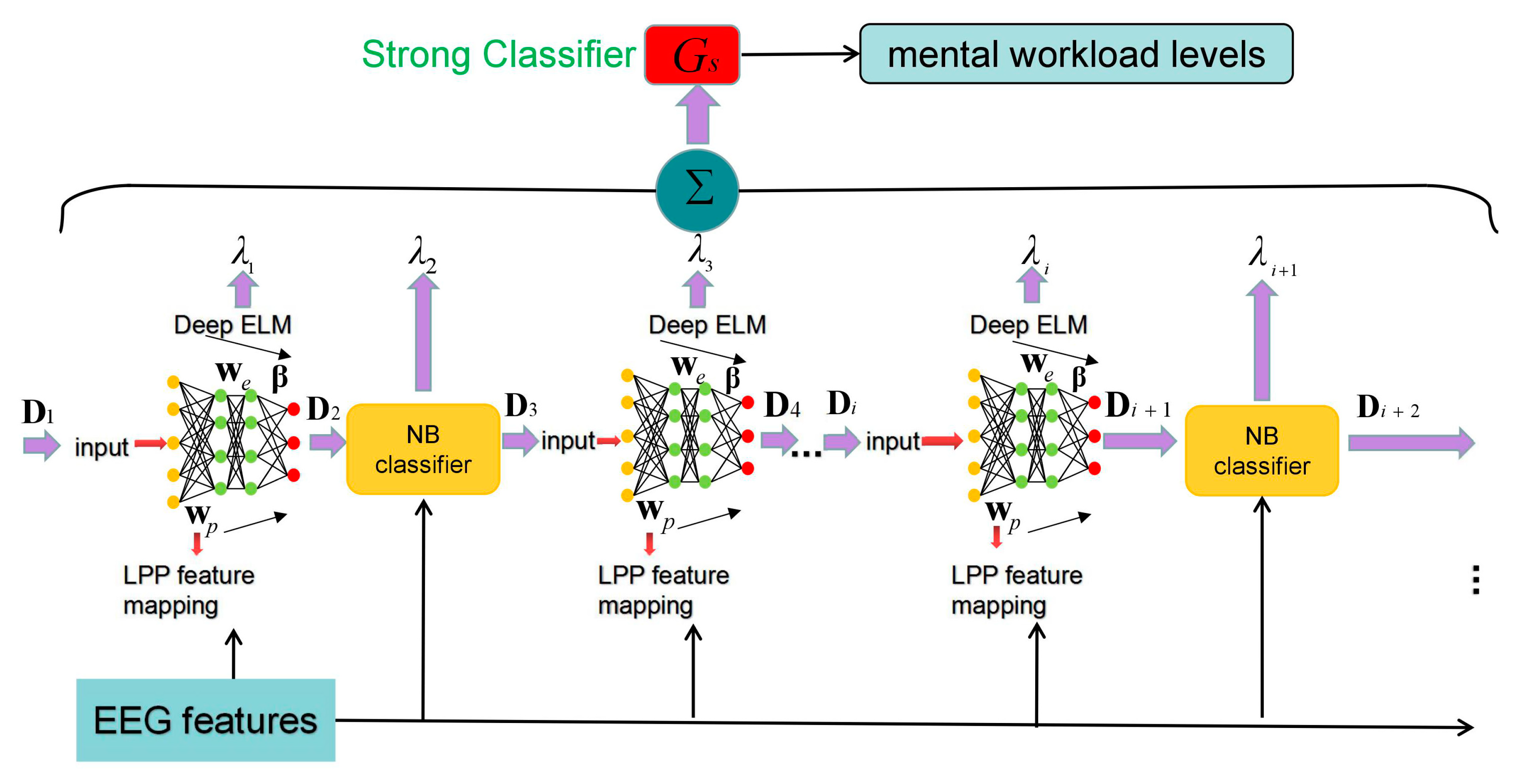
To further improve the generalization capability of the Adaboost ELM classifier on a specific participant, we adopted heterogeneous weak classifiers and the deep learning principle. The architecture of the proposed method termed as heterogeneous ensemble ELM (HE-ELM) is illustrated in Figure 4.

Figure 4. Framework of the heterogeneous extreme learning machine (ELM) ensemble for individual dependent mental workload (MW) classification.

On one hand, the Naive Bayesian (NB) model was used as alternative weak classifiers to improve the diversity of the ensemble committee. The motivation behind this lies in two aspects: (1) The input weights of all member ELMs are randomly determined from a uniform distribution and it may lead to similar hidden-neuron properties across two weak classifiers; (2) the mechanism of the inference functionality for the Bayesian model is inherently different from the classical ELM and thus facilitates a heterogeneous classifier ensemble.

By setting different values of the class prior probability, we obtained diverse Bayesian models. For ELMs, we implemented different activation functions and hidden neuron numbers. To this end, Bayesian and ELM models with different hyper-parameters can produce a group of dissimilar decision boundaries. The overall error of the strong classifier can be reduced after integrating all heterogeneous models.

By denoting the maximum number of the iteration as $M$, the whole ensemble process builds $M$ weak classifiers, where the $M$ classifiers consist of $T$ NB models (denoted by $G_t(\cdot ),0<t\le T$) and $K$ ELMs (denoted by $G_k(\cdot ),0<k\le K$) with $T+K=M$. According to Equation (3), the output of each ELM can be expressed as

$$G_k({\mathbf{x}}_i)={\displaystyle \sum _{j=1}^S{\mathsf{\beta }}_j\cdot p(}{\mathbf{w}}_j\cdot {\mathbf{x}}_i+{\mathbf{b}}_j),i=1,2,\dots ,\tilde{S}$$

(12)

The prediction of the NB model is computed as

$$G_t({\mathbf{x}}_i)=\underset{C_k}{\arg \max }P({\widehat{\mathbf{y}}}_i=C_k){\displaystyle \prod _{i=1}^{\tilde{S}}P({\mathbf{x}}_i={\mathbf{x}}_i^{(test)}|{\widehat{\mathbf{y}}}_i=C_k)}$$

(13)

In Equation (13), ${\mathbf{x}}_i^{(test)}$ and $C_k$ denote the input instance and the label of class $k$ with $k=1,2,\dots ,K$, respectively. By incorporating ${\mathbf{y}}_s$ in Equation (11), the classification accuracy of the strong classifier $G_s(\cdot )$ generated in each iteration is defined as

$${\alpha }_s=1-U({\mathbf{y}}_i\ne {\mathbf{y}}_s)/N$$

(14)

where $U(\cdot )$ represents the function for measuring the number of misclassification EEG data points in all $N$ instances. Then, the member classifier $G_m(\cdot )$ in the $m^{th}$ iteration is selected by

$$G_m({\mathbf{x}}_i)=\{\begin{array}{l}{G}_k({\mathbf{x}}_i),\begin{array}{cc}& {\alpha }_s>{\alpha }_{s-1}\end{array}\\ G_t({\mathbf{x}}_i),\begin{array}{cc}& {\alpha }_s<{\alpha }_{s-1}\end{array}\end{array}$$

(15)

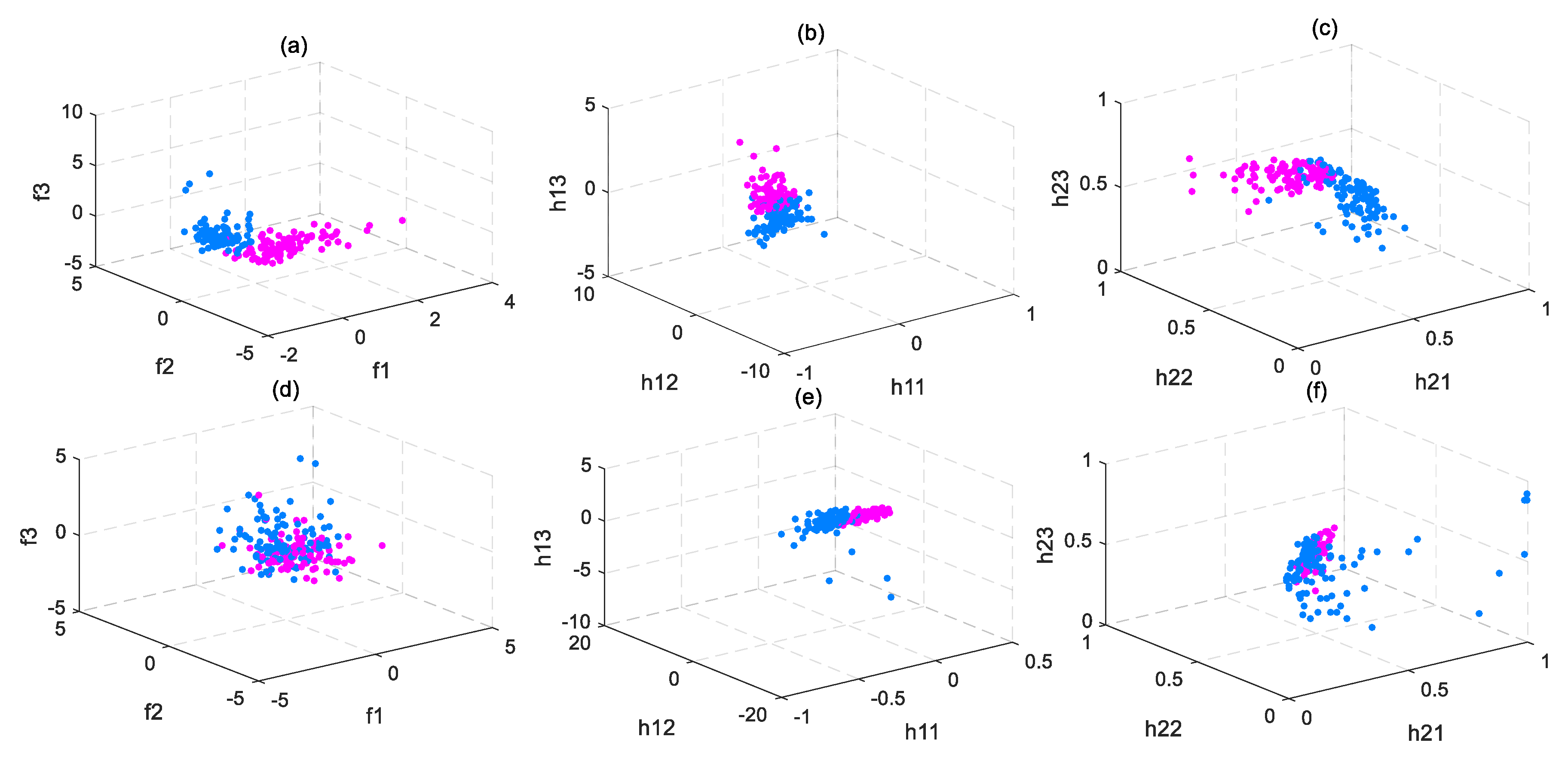
In addition, a deep network structure was applied in each member ELM and NB model aimed at finding high-level EEG feature representations. We add a new abstraction layer to the member classifier in which the network weights are trained by using local preserving projection (LPP) that preserves the local geometrical properties of the EEG data distribution [49,50]. Let denote the input weight as a transformation matrix $\mathbf{A}$ to map EEG feature vectors ${\mathbf{x}}_i\in R^q$ to a feature abstraction vector ${\mathbf{f}}_i\in R^l$, i.e.,

$${\mathbf{f}}_i={\mathbf{A}}^T{\mathbf{x}}_i,i=1,2,\dots ,\tilde{S}.$$

(16)

By creating an adjacent graph between ${\mathbf{x}}_i$ and ${\mathbf{x}}_j$, the entry $e_{ij}$ of edge matrix $\mathbf{E}$ is computed by using the Gaussian kernel with the width parameter $t>0$,

$$e_{ij}=\exp (-{\Vert {\mathbf{x}}_i-{\mathbf{x}}_j\Vert }_2^2/t)$$

(17)

The input weight $\mathbf{A}$ of the deep ELM network can be trained by solving the following linear equation system,

$${\mathbf{XLX}}^{\mathrm{T}}\mathbf{a}=\lambda {\mathbf{XDX}}^{\mathrm{T}}\mathbf{a}.$$

(18)

where $\mathbf{X}={[{\mathbf{x}}_1,{\mathbf{x}}_2,\dots ,{\mathbf{x}}_{\tilde{S}}]}^T$, $\mathbf{D}$, and $\mathbf{L}=\mathbf{D}-\mathbf{E}$ are the input sample array, the diagonal matrix computed from $d_{ii}={\displaystyle \sum _j{e}_{ij}}$, and the Laplacian matrix, respectively. By denoting the solution of Equation (18) as column vectors ${\mathbf{a}}_0,{\mathbf{a}}_1,\dots ,{\mathbf{a}}_{l-1}$, the input weight of a deep ELM is $\mathbf{A}=[{\mathbf{a}}_0,{\mathbf{a}}_1,\dots ,{\mathbf{a}}_{l-1}]$.

To this end, the output of each deep ELM classifier can be formulized as

$${\tilde{G}}_k({\mathbf{x}}_i)={\displaystyle \sum _{j=1}^S{\mathsf{\beta }}_j\cdot p[{\mathbf{w}}_j\cdot ({\mathbf{A}}^T{\mathbf{x}}_i)+{\mathbf{b}}_j]},i=1,2,\dots ,\tilde{S}$$

(19)

For the NB model, the dimensionality of the EEG feature vectors have been reduced and its output is computed as

$$G_t({\mathbf{f}}_i)=\underset{C_k}{\arg \max }P({\widehat{\mathbf{y}}}_i=C_k){\displaystyle \prod _{i=1}^{\tilde{S}}P({\mathbf{f}}_i={\mathbf{f}}_i^{(test)}|{\widehat{\mathbf{y}}}_i=C_k)}.$$

(20)

It is noted the final strong classifiers are generated in the last iteration of each ensemble learning process on the training set from a single participant, i.e., participant-dependent classifiers are built for MW recognition.

Table 4 lists the pseudo codes for the proposed HE-ELM algorithm [46], where the dimension required to reduce the dimension of the matrix is $D$, the prior probability of the NB model is $P_{pri}$, the output of the strong classifier is ${\mathbf{Y}}_s$ and the dimensionally reduced input matrix is ${\mathbf{X}}_L$. It is noted in the initial iteration that the weak classifier ${\tilde{G}}_1(\cdot )$ was constructed by an ELM model. If the performance of the newly-added classifier, i.e., another ELM ${\tilde{G}}_2(\cdot )$, in the second iteration is lower than the current strong classifier, we rebuild ${\tilde{G}}_2(\cdot )$ and compare it against a weak NB model according to Equation (20). In the case that the highest performance of ${\tilde{G}}_2(\cdot )$ is achieved, the next iteration is carried out. Each subsequent iteration repeats such a computational process until the final strong classifier is generated.

Table 4. The pseudo codes for training and testing a heterogeneous ensemble extreme learning machine (HE-ELM) classifier.

HE_ELM$\left(\mathbf{X},\mathbf{Y},p(\cdot ),S,D,P_{pri},M\right)$
1	Compute the input weights $\mathbf{A}$ via Equation (18)
2	${\mathbf{X}}_L={\mathbf{A}}^T\mathbf{X}$
3	${\mathbf{D}}_1={[1/N,1/N,\dots ,1/N]}^T$, ${\alpha }_s^{(0)}=0$
4	ELM_train $(\{{\mathbf{X}}_L,\mathbf{Y}\},p,S)$
5	return${\tilde{G}}_1(\cdot )$
6	for$m$ = 1 to $M$
7	${\tilde{e}}_m={\displaystyle \sum _{i=1}^N{\mathbf{D}}_m(i)}I[{\tilde{G}}_m({\mathbf{x}}_i)\ne {\mathbf{y}}_i]$
8	${\tilde{\lambda }}_m=1/2\ln [(1-{\tilde{e}}_m)/{\tilde{e}}_m]$
9	Update ${\mathbf{D}}_{m+1}$ according to Equation (10)
10	${\tilde{G}}_s^{(m)}(\cdot )=\mathrm{sign}[{\displaystyle {\sum }_{z=1}^m{\tilde{\lambda }}_z{\tilde{G}}_z(\mathbf{X})}]$
11	Compute ${\alpha }_s^{(m)}$ on ${\tilde{G}}_s^{(m)}(\cdot )$ via Equation (14)
12	if ${\alpha }_s^{(m)}\le {\alpha }_s^{(m-1)}$
13	Compute ${\tilde{G}}_{m+1}(\cdot )$ according to Equation (20)
14	else ELM_train $({\mathbf{X}}_L,\mathbf{Y},p,S)$
15	return a deep ELM ${\tilde{G}}_{m+1}(\cdot )$
16	${\mathbf{Y}}_s={\tilde{G}}_s^{(M)}(\mathbf{X})=\mathrm{sign}[{\displaystyle {\sum }_{z=1}^m{\tilde{\lambda }}_z{\tilde{G}}_z(\mathbf{X})}]$
17	return${\mathbf{Y}}_s$

3. Results

To validate the proposed HE-ELM method for MW classification, two cases of the data-splitting paradigms were designed in Figure 5. In Case 1, the MW classifier was trained and tested across each EEG feature set of a participant. Case 1 employed an individual dependent paradigm. For each participant, two-session EEG data of 3600 instances were divided into training and testing sets of 2400 and 1200 instances, respectively. For Case 2, the training and testing datasets were generated following an individual independent principle. That is, all neurophysiological features sets of eight participants were integrated into a single database with 28,800 EEG instances. Then, the hold-out method was applied to determine two mutually exclusive training and testing sets with the sample size of 19,200 and a testing size of 9600, respectively. All algorithms were trained and tested on Matlab^® 2016a software and performed via an Intel core i5-6200U CPU @ 1.30GHz PC with Windows 7^® operating system and 4 GB of RAM. Among them, Matlab^® 2016a software is developed and supplied by MathWorks Company in Natick, Massachusetts, USA. The PC device is produced by ASUS in Taipei, Taiwan. The ANN algorithm for performance comparison was realized by the neural network toolbox of Matlab (Ver. 9.0).

Figure 5. Training and testing data splits for mental workload classifiers: (a) Case 1: For each participant, two-session EEG data of 3600 instances were divided into training and testing sets of 2400 and 1200 instances, respectively; (b) Case 2: Two mutually exclusive training and testing sets with the sample size of 19,200 and a testing 9600 were used.

3.1. Model Selection for HE-ELM

Figure 6 depicts the training and testing accuracy of the classical ELM classifier under Case 1 and Case 2 with a different number of the hidden neurons employed. Three different activation functions of the ELM, i.e., hard limit, sigmoid, and sine functions, were investigated. In the training phase of both cases, we found that the sigmoid and the sine functions possess the fastest and the lowest convergence rates respectively. The training accuracy of the ELM monotonously rises under all activation functions and the perfect training performance is achieved when a sufficient amount of hidden neurons is adopted. The testing accuracy of the sine function for both cases achieved the lowest value, and is just slightly better than random guess. The highest testing accuracy under the hard limit function in Figure 6a–c outperforms that of under sigmoid activation function. Specifically, in Figure 6d the hard limit function is slightly better. The observation indicates the effectiveness of the activation function for the ELM model is related to the size of the EEG feature set.

Figure 6. Training and testing accuracy of the ELM classifier under Case 1 (a–c) and Case 2 (d) vs. the variation of the number of hidden neurons. For Case 1, the performance of ELM on the EEG feature sets from participant S1, S2 and S3 is presented. The labels of hardlim, sigmoid, and sine indicating the hard limit, sigmoid, and sine activation function were employed, respectively.

The number of the ELM hidden nodes under the optimal performance for each participant is summarized in Table 5. We found that the optimal number of hidden nodes for training is much higher than that for testing. It implies the perfect training performance is achieved for complex network structures while a good generalization capability corresponds to a simpler structure.

Table 5. Number of hidden nodes, training and testing accuracy under the optimal classification of ELM classifier in each subject’s EEG feature set for training and testing.

Subjects	Size of Hidden Neurons		Accuracy		Activation Function
	Training	Testing	Training	Testing
S1	1621	261	1.0000	0.8967	hardlim
	1421	331	1.0000	0.9117	sigmoid
	2191	1541	1.0000	0.5517	sine
S2	1581	461	1.0000	0.9333	hardlim
	1321	281	1.0000	0.9525	sigmoid
	2081	211	1.0000	0.5392	sine
S3	1881	701	1.0000	0.8650	hardlim
	1791	351	1.0000	0.8808	sigmoid
	2141	1271	1.0000	0.5417	sine
S4	2001	651	1.0000	0.7367	hardlim
	2011	391	1.0000	0.7600	sigmoid
	2141	2061	1.0000	0.5492	sine
S5	1921	211	1.0000	0.8200	hardlim
	1881	221	1.0000	0.8325	sigmoid
	2171	1771	1.0000	0.5425	sine
S6	1611	391	1.0000	0.8942	hardlim
	1581	511	1.0000	0.9142	sigmoid
	2141	1851	1.0000	0.5375	sine
S7	1671	471	1.0000	0.9108	hardlim
	1671	231	1.0000	0.9167	sigmoid
	2171	1371	1.0000	0.5333	sine
S8	1761	491	1.0000	0.8317	hardlim
	1851	571	1.0000	0.8558	sigmoid
	2171	491	1.0000	0.5492	sine

In Figure 7, the average computational cost for training and testing an ELM classifier is presented. It is shown both of the training and testing time is positively correlated with increase of the number of hidden nodes. The time cost monotonously rises under all activation functions for two cases and the testing time duration is much smaller than that for the training. By observing the line plots, the computational burden under Case 1 is less than that under Case 2 because of a smaller sample size. We can note that the testing time under hard limit function achieves the least value in Figure 7b,d,f,h. There is no obvious difference for sine and sigmoid functions in Figure 7b,d,f under Case 1. It is noted the testing time of the ELM classifier under sine function achieves the highest value in Figure 7h while the time cost across three activation functions in the training stage does not significantly vary.

Figure 7. Training and testing time of an ELM classifier: (a,b) Case 1: Training and testing time for subjects (a,b) S1, (c,d) S2, and (e,f) S3. Case 2: (g,h) Training and testing time on the datasets from all subjects.

In order to select the optimal model structure for the proposed HE-ELM, we investigated its performance under different values for the number of the iterations in Table 6. The shallow ELM weak classifier was used to reduce the training time. For simplicity, the individual-dependent MW classifiers shared the same network structure. The optimal structure of the ELM weak classifier is shown in Table 7. It is shown the hardlim function with 201 hidden neurons is the best case. By comparing the two tables, it is observed that the ensemble ELM approach improves the accuracy by 1.43% against an optimally-trained ELM.

Table 6. The HE-ELM with shallow ELM weak model for Case 2.

Number of Iterations	Accuracy
10	0.6683
20	0.6694
30	0.6773
40	0.6846
41	0.6854
42	0.6857
43	0.6847
44	0.6848
45	0.6859
46	0.6865
47	0.6850
48	0.6853
49	0.6855
50	0.6852
60	0.6844

Note: The maximum value is marked in the bold type.

Table 7. The ELM performance for Case 2.

Number of Hidden Neurons	Accuracy	Activation Function
201	0.6722	hardlim
301	0.6683	sigmoid
1301	0.5120	sine

Note: The optimal value in each column is marked in bold.

3.2. Accuracy Comparison between HE-ELM and Different MW Classifiers

We implemented the proposed HE-ELM to generate participant-specific MW classification testing accuracy. In Figure 8, the performance of all subjects for HE-ELM is compared against the deep ELM and the classical ELM under an optimal network structure. The histogram indicates the accuracy of the HE-ELM, and the ELM classifiers achieve the highest and the lowest values, respectively. It is shown that the performance improvement of the HE-ELM is particularly significant for subjects D and E. The number of the iterations and the proportion of the weak classifiers of each type are listed in Table 8. From the Table, it is observed that the number of iterations and the percentages on deep ELM and NB classifiers are different across 8 subjects. The proportion of ELM is much larger than that of NB. In particular, for subject S6, only a single iteration was performed. It is because the first weak classifier had already achieved an optimal classification performance while the Adaboost algorithm cannot further improve accuracy.

Figure 8. Testing accuracy of individual-specific MW classifiers for HE-ELM, deep ELM, and classical ELM.

Table 8. Individual-dependent classification committee of the HE-ELM.

Subject Index	Number of Iterations	Number and Proportion of Deep ELM Classifiers	Number and Proportion of NB Classifiers
S1	6	4 (66.6%)	2 (33.3%)
S2	6	4 (66.6%)	2 (33.3%)
S3	11	10 (90.9%)	1 (0.9%)
S4	6	6 (100%)	0 (0%)
S5	6	4 (66.6%)	2 (33.3%)
S6	1	1 (100%)	0 (0)
S7	4	2 (50%)	2 (50%)
S8	11	9 (81.8%)	2 (18.1%)

Next, we compared the performance of the HE-ELM classifier against the classical ELM, K-nearest neighbor (KNN), artificial neural network with single hidden layer (ANN), denoising autoencoder (DAE), logistic regression (LR), Adaboost based on the decision tree, stacked denoising autoencoder (SDAE), and NB MW prediction models. In addition, the LPP-based feature mapping is adopted to produce eight deep-structured classifiers denoted by deep ELM, LPP-KNN, LPP-ANN, LPP-DAE, LPP-LR, LPP-AD, LPP-SDAE, and LPP-NB.

In Figure 9, we examine the performance of the classifiers used for comparison with different hyper-parameters on four representative subjects. It is noted the NB and LR based model have none of the hyper-parameters controlling the model complexity and thus have not been analyzed in the figure. From Figure 9, it is shown the testing accuracy of ELM, KNN, deep ELM, and LPP-KNN classifier arises with the model complexity. Specifically, the maximum testing accuracy of deep ELM is higher than that of ELM in all four subjects. On the other hand, the optimal performance of LPP-KNN is better than that of KNN. Compared with ANN, LPP-ANN achieves better optimal performance while the accuracy of the DAE model is similar to that of LPP-DAE.

Figure 9. MW classification testing accuracy on 4 subjects for (a) ELM; (b) K-nearest neighbor (KNN); (c) artificial neural network with single hidden layer (ANN); (d) denoising autoencoder (DAE); (e) deep ELM; (f) local preserving projection (LPP)-KNN; (g) LPP-ANN and (h) LPP-DAE vs. different model hyper-parameters. The hyper-parameters of ELM, ANN, DAE, deep ELM, LPP-ANN and LPP-DAE are the number of hidden neurons. The hyper-parameter of KNN and LPP-KNN is the number of the nearest neighbors (denoted by k).

The optimal testing classification accuracy generated by 17 classifiers is illustrated in Figure 10 via box plots. For all methods, HE-ELM and LPP-KNN achieve the best and the worst average accuracy, respectively. The classification performance of the MW classifiers except for KNN is improved when using LPP feature leaning. It implies the generalization capability of shallow classifiers can be enhanced via a layer of intermediate feature representation. The mean of accuracy, precision, and recall of the MW classifiers on eight subjects is shown in Table 9. The table specifically presents the difference in the classification performance of the 17 MW classifiers. It is shown that the mean values of the three evaluation indicators of HE-ELM are all the highest while the standard deviation of the accuracy of HE-ELM is the lowest among all MW classifiers. In particular, LPP-KNN has the lowest mean of accuracy and recall while the average recall of the NB model is the lowest.

Figure 10. Box plots for 17 classifiers performance for individual dependent MW classification. The statistics in each column data are computed from the testing classification accuracy for all eight subjects.

Table 9. Classification performance of the MW classifiers for all eight subjects.

MW Classifier	Mean			s.d.
	Accuracy	Precision	Recall	Accuracy	Precision	Recall
ELM	0.878	0.8763	0.8797	0.0609	0.0582	0.0662
DAE	0.8767	0.8758	0.8804	0.0616	0.0688	0.0618
ANN	0.8182	0.8177	0.8235	0.1124	0.1126	0.1048
NB	0.7778	0.8435	0.6785	0.1002	0.0348	0.2345
LR	0.9124	0.9135	0.9119	0.0404	0.0445	0.0361
KNN	0.8056	0.7911	0.8416	0.0758	0.0921	0.0861
SDAE	0.8876	0.8862	0.8889	0.0561	0.0497	0.0759
Adaboost	0.8803	0.8785	0.8831	0.0653	0.0655	0.0644
Deep ELM	0.928	0.9314	0.9237	0.0423	0.0379	0.0513
LPP-DAE	0.9062	0.9073	0.9087	0.055	0.0672	0.0621
LPP-NB	0.8885	0.9158	0.8564	0.0918	0.0692	0.1505
LPP-LR	0.9282	0.9293	0.9275	0.0391	0.0425	0.0406
LPP-ANN	0.9279	0.9249	0.9314	0.0425	0.0427	0.0438
LPP-KNN	0.7711	0.7795	0.8062	0.1153	0.1431	0.1124
LPP-AD	0.9322	0.9272	0.9392	0.0389	0.0383	0.0485
LPP-SDAE	0.8798	0.8781	0.8917	0.1214	0.1304	0.0996
HE-ELM	0.9384	0.9348	0.9433	0.0386	0.0401	0.0372

Note: The minimum and maximum values in each column are underlined and marked with the bold type, respectively.

The results of two-tailed test between HE-ELM and other 16 MW classifiers are listed in Table 10. It is found that HE-ELM has a significant improvement in accuracy compared to other classifiers except for LPP-SDAE. For precision and recall values, HE-ELM are comparable with six deep structure classifiers generated based on LPP-based feature mapping except for LPP-KNN and LPP-ANN. In general, the accuracy of the HE-ELM is superior to most pattern classifiers and is comparable with the advanced deep learning method.

Table 10. Results of two-tailed t-test comparing HE-ELM with 16 other MW classifiers.

MW Classifier	Accuracy		Precision		Recall
HE-ELM vs. ELM	t = 5.9112	p = 0.0006	t = 5.8759	p = 0.0006	t = 4.7131	p = 0.0022
HE-ELM vs. DAE	t = 6.1614	p = 0.0005	t = 3.9249	p = 0.0057	t = 4.3161	p = 0.0035
HE-ELM vs. ANN	t = 2.9515	p = 0.0213	t = 2.8119	p = 0.0261	t = 3.4224	p = 0.0111
HE-ELM vs. NB	t = 6.8741	p = 0.0002	t = 8.0088	p = <0.0001	t = 3.6874	p = 0.0078
HE-ELM vs. LR	t = 5.3195	p = 0.0011	t = 4.1021	p = 0.0046	t = 6.3117	p = 0.0004
HE-ELM vs. KNN	t = 4.8887	p = 0.0018	t = 4.2814	p = 0.0036	t = 3.1671	p = 0.0158
HE-ELM vs. SDAE	t = 5.6262	p = 0.0008	t = 4.6278	p = 0.0024	t = 3.0531	p = 0.0185
HE-ELM vs. Adaboost	t = 4.9370	p = 0.0017	t = 4.8494	p = 0.0019	t = 4.9756	p = 0.0016
HE-ELM vs. Deep ELM	t = 3.2168	p = 0.0147	t = 0.7537	p = 0.4756	t = 1.9432	p = 0.0931
HE-ELM vs. LPP-DAE	t = 3.6243	p = 0.0085	t = 1.5724	p = 0.1599	t = 2.490	p = 0.0416
HE-ELM vs. LPP-NB	t = 2.1636	p = 0.0472	t = 1.504	p = 0.1763	t = 1.8093	p = 0.1133
HE-ELM vs. LPP-LR	t = 9.8706	p = <0.0001	t = 1.7792	p = 0.1184	t = 3.161	p = 0.0159
HE-ELM vs. LPP-ANN	t = 6.8041	p = 0.0003	t = 3.9848	p = 0.0053	t = 3.2927	p = 0.0132
HE-ELM vs. LPP-KNN	t = 4.9900	p = 0.0016	t = 3.5837	p = 0.0089	t = 3.8710	p = 0.0061
HE-ELM vs. LPP-AD	t = 4.2052	p = 0.004	t = 1.6532	p = 0.1423	t = 0.6349	p = 0.5455
HE-ELM vs. LPP-SDAE	t = 1.6693	p = 0.1389	t = 1.4507	p = 0.1902	t = 1.9213	p = 0.0961

Note: The significant cases with value p < 0.05 are marked with the bold type.

The number of hidden layer nodes, the k values for KNN, the number of weak classifiers, and the proportion of deep ELM classifiers for each subject is summarized in Table 11. As we noted, the number of hidden neurons under the optimal classification of ELM and deep ELM were lower than that of ANN and LPP-ANN, respectively. However, the DAE-based MW classifier possessed the simplest structure with a minimum number of hidden nodes. For LPP-AD, the average number of iterations was lower than Adaboost. The number of neurons on the two hidden layers of LPP-SDAE was less than that of SDAE. For HE-ELM, 77.8% weak classifiers in average were constructed via deep ELMs. The remaining 22.2% was generated by NB models. For all eight subjects, the optimal structure hyper-parameters varied significantly, which indicates an individual-specific MW classifier is necessary.

Table 11. Optimal structure hyper-parameters of the MW classifiers.

Subject index	ELM	DAE	ANN	KNN	SDAE		Adaboost	Deep ELM	LPP-DAE	LPP-ANN	LPP-KNN	LPP-SDAE		LPP-AD	HE-ELM
					1	2						1	2
S1	331	121	1261	23	90	150	58	301	121	61	13	130	30	1	6 (66.6%)
S2	281	351	551	6	110	150	64	101	291	231	30	50	70	19	6 (66.6%)
S3	351	111	1041	4	130	130	51	321	111	461	12	70	130	29	11 (90.9%)
S4	391	101	451	76	150	130	62	161	101	371	35	70	130	65	6 (100%)
S5	221	151	101	14	130	10	63	161	151	71	38	130	130	21	6 (66.6%)
S6	511	261	421	10	130	10	64	131	261	361	27	30	110	17	1 (100%)
S7	231	61	1051	35	130	90	60	201	191	931	95	50	90	18	4 (50.0%)
S8	571	121	951	36	110	150	65	161	231	741	16	110	90	23	11 (81.8%)
Average	361	160	729	26	58	48	29	192	182	403	33	38	46	11	6 (77.8%)

Note: The hyper-parameters of ELM, ANN, DAE, SDAE, deep ELM, LPP-SDAE, LPP-ANN and LPP-DAE are the number of hidden neurons. The hyper-parameter of KNN and LPP-KNN is the number of the k nearest neighbors. The hyper-parameter of Adaboost and LPP-AD is the number of iterations. The hyper-parameters of HE-ELM are the number of weak classifiers and the proportion of deep ELM classifiers. In particular, “1” represents the first hidden layer and “2” represents the second hidden layer.

3.3. Computational Cost Comparison

The average CPU time for training and testing a MW classifier on the EEG feature set for a single subject is shown in Table 12. From the table, the LPP-NB and Adaboost achieved the lowest and the highest computational burden. Adaboost had the highest computational cost mainly because it required a large number of iterations on the data set of this experiment. The main reason for the high computational overhead of HE-ELM is that HE-ELM method tried to select suitable weak classifiers in each iteration and each weak classifier can be either an ELM or a NB-based classification model. Thus, the shortcoming of HE-ELM is its high computational cost in training although it effectively improves the MW classification accuracy compared to the classical ELM algorithm. For other classifiers, using LPP for dimensionality reduction can significantly reduce the computational cost. A high computational burden can be observed in the machine learning approaches using gradient decent optimization, e.g., DAE, SDAE, and ANN.

Table 12. Average CPU time (in sec) for training and testing a MW classifier with a EEG feature set for a single subject. The standard deviation (denoted by s.d.) and mean values are calculated across 50 repeated trials.

Classifier	Training		Testing
	Mean	s.d.	Mean	s.d.
ELM	0.3045	0.0273	0.5744	0.0280
NB	0.1694	0.1795	0.0243	0.0155
KNN	0.0162	0.0396	0.5725	0.0322
DAE	1.7840	0.1250	0.1740	0.0379
ANN	3.2071	1.1786	0.0356	0.0126
LR	3.3983	0.1305	0.0168	0.0359
SDAE	11.275	0.6258	0.1325	0.0231
Adaboost	31.504	0.5583	0.0234	0.0211
Deep ELM	0.2162	0.0447	0.1891	0.0292
LPP-NB	0.0371	0.0117	0.0090	0.0141
LPP-KNN	0.0103	0.0112	0.1279	0.0148
LPP-DAE	1.8040	0.0810	0.1690	0.0240
LPP-ANN	1.3790	0.4569	0.0624	0.0221
LPP-LR	0.0440	0.0186	0.0044	0.0151
LPP-SDAE	12.142	1.3520	0.1277	0.0323
LPP-AD	5.6332	0.0651	0.0109	0.0105
HE-ELM	9.030	0.1970	0.2552	0.0709

Note: The minimum and maximum values in each column are underlined and marked with the bold type, respectively.

3.4. Visualization of the Intermediate EEG Feature Representations

The intermediate EEG features abstracted in hidden layers of the deep ELM in HE-ELM are shown in Figure 11. To facilitate visualizing the abstraction distribution, three representative hidden variables from the EEG dataset of two subjects were selected to be illustrated in 3-D scatter plots. It was shown the abstraction vectors corresponding to low and high MW levels can be clearly distinguished after EEG features were properly mapped via hidden units of the weak classifier in HE-ELM. In the 1st hidden layer, the 137 EEG features (the first three features are shown in Figure 11a,d) were fused into 27 hidden variables (the first three variables are plotted in Figure 11a,b,d,e). The first abstraction layer of the neural network of Deep ELM was added by LPP method. It is noted the abstraction vectors in Figure 11c,f are more concentrated than that shown in Figure 11a,d. It implies the deep architecture is helpful for salient information fusion when EEG feature from multiple domains are available.

Figure 11. 3-D scatter plots of the EEG feature abstractions for low and high MW classes extracted from EEG features from two subjects, (a–c) S2, (d–f) S3. Subfigures (a,d) visualize the EEG features; Subfigures (b,e) depict the outputs of the first hidden layer in HE-ELM; Subfigures (c,f) show the outputs of the activations in the second hidden layer.

4. Discussion

The proposed HE-ELM for MW assessment integrates ELMs with classical NB models to form a heterogeneous strong classifier. To ensure the effectiveness of the integrated ensemble committee, the hyper-parameters of each weak classifier were set to be different. On the premise of ensuring the model diversity, the iteration programming was performed until it reached the highest classification performance. To find the optimal structure of the HE-ELM, we first implemented the Adaboost-ELM and observed that the ELM ensemble outperformed the classical ELM when a moderate amount of iterations was used. However, the performance improvement was marginal since the data distribution of the EEG features shared a great individual difference. Therefore, we implemented a deep ELM network structure to find the stable EEG feature representation combined with an individual-specific (or subject-dependent) classification paradigm.

According to the existing literature related to the machine-learning-based EEG classification, a group of effective classifiers were validated such as NB, ANN, KNN algorithm, DAE, and LR. We compared the HE-ELM against the above approaches and the former achieved the highest performance. Several observations were found when tackling high dimensional EEG features. The KNN method easily over-fits when the k value is set too small [51]. On the other hand, its computational complexity increases with a large k used. The performance of the ANN with a single hidden layer is unstable because its shallow structure is incapable of fusing the noised EEG features. By adding noised training samples to make the output similar to the input signal [52], DAE achieves better performance than ANN. The LR model maps the range of the original output results to an interval of (0,1) by a logistic sigmoid function [53]. However, the lack of the intermediate feature representation limits the adaptability of DAE and LR on individual-dependent EEG feature sets.

In the literature, Ayaz et al. measured operator MW in an unmanned aerial vehicle control task. Based on one-way repeated measures ANOVA analysis of the fNIRS data, significant differences between the MW indices corresponding to different task demands have been found [16]. In our previous work, the RBF-kernel and the linear-kernel based SVM were utilized for assessing binary MW [54]. The average classification accuracy was obtained from 0.7912 to 0.9317. An adaptive Stacked Denoising AutoEncoder (A-SDAE) was used in the binary MW classification problem in [21]. By employing the dimensionality of EEG features of 55, the mean value of accuracy on seven subjects was 0.8579. In the current work, the average accuracy of the HE-ELM algorithm finally obtained on all eight subjects was 0.9384. The improvement of the HE-ELM performance with ensemble learning principle was partially found. Because the training and testing environment was different, it is difficult to achieve strict performance analysis.

Although the HE-ELM improves the performance of the standard ELM as well as the LPP-based deep ELM, the main limitation is that the technology is an offline simulation and its training time cost is significantly higher than single, shallow machine learning models. In particular, the classification method proposed in this paper is for offline simulation and was not tested in an online fashion. It leads to a limitation that the proposed algorithm requires the entire dataset and cannot be scheduled in real time. Moreover, the training time cost is significantly higher than single, shallow machine learning models and this problem may impair the effectiveness for retraining the MW classifier on the EEG data from a novel operator of the human–machine system. When the size of sample is too large, the number of required iterations for HE-ELM will increase since more suitable weak classifiers need to be generated. However, the computational cost of HE-ELM was mainly introduced in the training stage. When the trained HE-ELM model is used for testing unseen EEG feature vectors, the required time is still comparable to shallow MW classifiers. It is also noted that an additional hyper-parameter of HE-ELM was introduced, i.e., the optimal number of iterations. By observing Table 11, we found it affects the value of the accuracy when individual-specific MW classifier ensemble was employed. The technical challenge of this paper is how to find the appropriate NB models to iterate with ELM models, so as to effectively improve the classification performance. In many cases, the selected NB model may reduce the classification performance of the final strong classifier. The other possible limitation is that the size of the training data is insufficient to achieve stable online performance. Therefore, it should be noted the accuracy cannot be guaranteed in online, real world application developments. In future work, the online MW recognition of the proposed method should be investigated and validated.

As a future direction, it is promising to investigate whether a generic MW classifier ensemble can be found for all individuals in an online fashion. It is noted that the fNIRS is an optical brain monitoring technique that has been used to evaluate MW in ecologically valid environments [16]. The merits of fNIRS are its low invasiveness for data acquisition and high reliability. However, the current fNIRS device is not suitable for monitoring all cortical areas while the time resolution of the acquired data need to be enhanced. The BCI-based MW assessment system that fuses both the EEG and fNIRS modalities is a promising solution. Such a hybrid system has been documented in Babiloni et al. [55]. The ensemble learning based approach such as our HE-ELM may be helpful for fusing features from two different domains. The possible obstacles can be the synchronicity of the EEG and fNIRS features, the higher computational burden, and the difference of the sampling frequency on two modalities when the online MW assessment is implemented.

5. Conclusions

In this paper, we present a new machine-learning based OFS evaluator, HE-ELM, to classify EEG features into binary levels of MW. Under an individual-specific modeling paradigm, the HE-ELM was constructed by heterogeneous deep ELM and NB weak classifiers. Two types of the member classifier structure were employed to enhance the diversity of the classification committee generated via the Adaboost algorithm. To find the proper hyper-parameters of the proposed ensemble model, the number of hidden nodes and the optimal activation function for HE-ELM were identified. To validate the effectiveness of HE-ELM, we introduced eight EEG feature sets via the hold-out method to build training and testing sets. The classical single, and shallow MW classifiers were employed for comparison on the classification accuracy and the computational cost. We found the HE-ELM model superior in improving the individual-specific accuracy of MW assessments although it is at the cost of the training burden. The HE-ELM algorithm in this paper is an offline simulation, but it may be possible to solve this problem in the future by combining it with fNIRS technology. The combined EEG and fNIRS hybrid system may have some disadvantages such as computational cost. In general, the combined EEG and fNIRS hybrid system is worth a try in the assessment of MW in the future.

References

- Giraudet, L.; Imbert, J.P.; Berenger, M.; Tremblay, S.; Causse, M. The neuroergonomic evaluation of human machine interface design in air traffic control using behavioral and EGG/ERP measures. Behav. Brain Res. 2015, 291, 246–253. [Google Scholar] [CrossRef] [PubMed]
- Sanjram, P.K. Attention and intended action in multitasking: An understanding of workload. Displays 2013, 32, 283–291. [Google Scholar] [CrossRef]
- Aricò, P.; Borghini, G.; Di, F.G.; Sciaraffa, N.; Babiloni, F. Passive BCI beyond the lab: Current trends and future directions. Physiol. Meas. 2018, 39, 1361–6579. [Google Scholar] [CrossRef] [PubMed]
- Byrne, E.A.; Parasuraman, R. Psychophysiology and adaptive automation. Biol. Psychol. 1996, 42, 249–268. [Google Scholar] [CrossRef]
- Cannon, J.; Krokhmal, P.A.; Lenth, R.V.; Murphey, R. An algorithm for online detection of temporal changes in operator cognitive state using real-time psychophysiological data. Biomed. Signal Process. Control 2010, 5, 229–236. [Google Scholar] [CrossRef]
- Cannon, J.; Krokhmal, P.A.; Chen, Y.; Murphey, R. Detection of temporal changes in psychophysiological data using statistical process control methods. Comput. Methods Programs Biomed. 2012, 107, 367–381. [Google Scholar] [CrossRef]
- Ting, C.; Mahfouf, M.; Nassef, A.; Linkens, D.; Panoutsos, G.; Niclkel, P.; Roberts, A.; Hockey, G.R.J. Real-time adaptive automation system based on identification of operator functional state in simulated process control operations. IEEE Trans. Syst. Man Cybern. Part A Syst. Hum. 2010, 40, 251–262. [Google Scholar] [CrossRef]
- Majumdar, K. Human scalp EEG processing: Various soft computing approaches. Appl. Soft Comput. 2011, 11, 4433–4447. [Google Scholar] [CrossRef]
- Gundel, A.; Wilson, G.F. Topographical changes in the ongoing EEG related to the diffificulty of mental tasks. Brain Topogr. 1992, 5, 17–25. [Google Scholar] [CrossRef]
- Wilson, G.F.; Fisher, F. Cognitive task classification based upon topographic EEG data. Biol. Psychol. 1995, 40, 239–250. [Google Scholar] [CrossRef]
- Aricò, P.; Borghini, G.; Di, F.G.; ColosimoA, P.S.; Babiloni, F. A passive brain-computer interface application for the mental workload assessment on professional air traffic controllers during realistic air traffic control tasks. Prog. Brain Res. 2016, 228, 295–328. [Google Scholar]
- Moon, B.S.; Lee, H.C.; Lee, Y.H.; Park, J.C. Fuzzy systems to process ECG and EEG signals for quantification of the mental workload. Inform. Sci. 2002, 142, 23–35. [Google Scholar] [CrossRef]
- Goro, O.; Satoru, T.; Naoki, S. Mental workloads can be objectively quantified in real-time using VOR (Vestibulo-Ocular Reflex). IFAC Pro. 2008, 41, 15094–15099. [Google Scholar]
- Ryu, K.; Myung, R. Evaluation of mental workload with a combined measure based on physiological indices during a dual task of tracking and mental arithmetic. Int. J. Ind. Ergonom. 2005, 35, 991–1009. [Google Scholar] [CrossRef]
- Dimitrakopoulos, G.N.; Kakko, I.; Dai, Z.X.; Lim, J.L.; De Souza, J.J.; Bezerianos, A.; Sun, Y. Task-Independent mental workload classification based upon common multiband EEG cortical connectivity. IEEE Trans. Neural Syst. Rehabil. Eng. 2017, 25, 1940–1949. [Google Scholar] [CrossRef]
- Ayaz, H.; Shewokis, P.A.; Bunce, S.; Izzetoglu, K.; Willems, B.; Onaral, B. Optical brain monitoring for operator training and mental workload assessment. Neuroimage 2012, 59, 36–47. [Google Scholar] [CrossRef]
- Subasi, A.; Ercelebi, E. Classification of EEG signals using neural network and logistic regression. Comput. Meth. Pro. Biomed. 2005, 78, 87–99. [Google Scholar] [CrossRef]
- Camps-Valls, G.; Bruzzone, L. Kernel-based methods for hyperspectral image classification. IEEE Trans. Geosci. Remote Sens. 2005, 43, 1351–1362. [Google Scholar] [CrossRef]
- Mazaeva, N.; Ntuen, C.; Lebby, G. Self-Organizing Map (SOM) model for mental workload classification. IEEE Conf. 2001, 3, 1822–1825. [Google Scholar]
- Antelis, J.M.; Gudiño-Mendoza, B.; Falcón, L.E.; Sanchez-Ante, G.; Sossa, H. Dendrite morphological neural networks for motor task recognition from electroencephalographic signals. Biomed. Signal Proces. 2018, 44, 12–24. [Google Scholar] [CrossRef]
- Yin, Z.; Zhang, J.H. Cross-session classification of mental workload levels using EEG and an adaptive deep learning model. Biomed. Signal Proces. 2017, 33, 30–47. [Google Scholar] [CrossRef]
- Zhao, G.Z.; Liu, Y.J.; Shi, Y.C. Real-Time assessment of the cross-task mental workload using physiological measures during anomaly detection. IEEE Trans. Hum. Mach. Syst. 2018, 48, 149–160. [Google Scholar] [CrossRef]
- Huang, G.B.; Zhu, Y.Q.; Siew, C.K. Extreme learning machine: A new learning scheme of feedforward neural networks. Proc. Int. Jt. Conf. Neural Netw. 2004, 2, 985–990. [Google Scholar]
- Huang, G.B. An insight into extreme learning machines: Random neurons, random features and kernels. Cogn. Comput. 2014, 6, 376–390. [Google Scholar] [CrossRef]
- Nicolas-Alonso, L.F.; Gomez-Gil, J. Brain Computer Interfaces: A Review. Sensors 2012, 12, 1211–1279. [Google Scholar] [CrossRef]
- Huang, G.B.; Siew, C. Extreme learning machine: RBF network case. ICARCV 2004, 2, 1029–1036. [Google Scholar]
- Huang, G.B.; Zhu, Q.Y.; Siew, C.K. Extreme learning machine: Theory and applications. Neurocomputing 2006, 70, 489–501. [Google Scholar] [CrossRef]
- Zhang, R.; Lan, Y.; Huang, G.B.; Xu, Z.B. Universal approximation of extreme learning machine with adaptive growth of hidden nodes. IEEE Trans. Neur. Net. Lear. 2012, 23, 365–371. [Google Scholar] [CrossRef]
- Qi, Y.; Zhou, W.D. Epileptic EEG classification based on extreme learning machine and nonlinear features. Epilesy Res. 2011, 96, 29–38. [Google Scholar]
- Huang, G.B.; Wang, D. Advances in extreme learning machines (ELM2011). Neurocomputing 2011, 74, 2411–2412. [Google Scholar] [CrossRef]
- Huang, G.B.; Song, S.J.; You, K.Y. Trends in extreme learning machines: A review. Neural Netw. 2015, 61, 32–48. [Google Scholar] [CrossRef]
- Shi, L.C.; Lu, B.L. EEG-based vigilance estimation using extreme learning machines. Neurocomputing 2013, 102, 135–143. [Google Scholar] [CrossRef]
- Zhang, J.; Yin, Z.; Wang, R. Recognition of mental workload levels under complex human-machine collaboration by using physiological features and adaptive support vector machines. IEEE Trans. Hum. Mach. Syst. 2015, 45, 200–214. [Google Scholar] [CrossRef]
- Sauer, J.; Nickel, P.; Wastell, D. Designing automation for complex work environments under different levels of stress. Appl. Ergon. 2013, 44, 119–127. [Google Scholar] [CrossRef]
- Sauer, J.; Wastell, D.G.; Hockey, G.R.J. A conceptual framework for designing micro-worlds for complex work domains: A case study on the cabin air management system. Comput. Hum. Behav. 2000, 16, 45–58. [Google Scholar] [CrossRef]
- Yin, Z.; Zhang, J. Identification of temporal variations in mental workload using locally-linear-embedding-based EEG feature reduction and support-vector-machine-based clustering and classification techniques. Comput. Methods Programs Biomed. 2014, 115, 119–134. [Google Scholar] [CrossRef]
- Slobounov, S.M.; Fukada, K.; Simon, R.; Rearick, M.; Ray, W. Neurophysiologicaland behavioral indices oftime pressure effects on visuomotor task performance. Cogn. Brain Res. 2000, 9, 287–298. [Google Scholar] [CrossRef]
- Fairclough, S.H.; Venables, L.; Tattersall, A. The inflfluence of task demand and learning on the psychophysiological response. Int. J. Psychophysiol. 2005, 56, 171–184. [Google Scholar] [CrossRef]
- Fairclough, S.H.; Venables, L. Prediction of subjective states from psychophysiology: A multivariate approach. Biol. Psychol. 2006, 71, 100–110. [Google Scholar] [CrossRef]
- Zhao, C.; Zhao, M.; Liu, J.; Zheng, C. Electroencephalogram and electrocardiograph assessment of mental fatigue in a driving simulator. Accid. Anal. Prev. 2012, 45, 83–90. [Google Scholar] [CrossRef]
- Yang, B.H.; Duan, K.; Fan, C.C.; Hu, C.X.; Wang, J.L. Automatic ocular artifacts removal in EEG using deep learning. Biomed. Signal Proces. 2018, 43, 148–158. [Google Scholar] [CrossRef]
- Borowicz, A. Using a multichannel wiener filter to remove eye-blink artifacts from EEG data. Biomed. Signal Process. 2018, 45, 246–255. [Google Scholar] [CrossRef]
- Manganotti, P.; Gerloff, C.; Toro, C.; Katsua, H.; Sadato, N.; Zhuang, P.; Leocani, L.; Hallet, M. Task-related coherence and task-related spectral power changes during sequential finger movements. Electroencephalogr. Clin. Neurophysiol. 1998, 109, 50–62. [Google Scholar] [CrossRef]
- Huang, G.B.; Wang, D.; Lan, Y. Extreme learning machines: A survey. Int. J. Mach. Learn. Cyb. 2011, 2, 107–122. [Google Scholar] [CrossRef]
- Huang, G.B.; Chen, L. Enhanced random search based incremental extreme learning machine. Neurocomputing 2008, 71, 3460–3468. [Google Scholar] [CrossRef]
- Cormen, T.H.; Leiserson, C.E.; Rivest, R.L.; Stein, C. Introduction to Algorithms, 2nd ed.; MIT Press: Cambridge, MA, USA, 2001. [Google Scholar]
- Freund, Y. An adaptive version of the boost by majority algorithm. Mach. Learn. 2001, 43, 293–318. [Google Scholar] [CrossRef]
- Friedman, J.H. Greedy function aproximation: A gradient boosting machine. Ann. Stat. 2001, 29, 1189–1232. [Google Scholar] [CrossRef]
- Zhang, Z.; Zhao, M.; Chow, T.W.S. Constrained large margin local projection algorithms and extensions for multimodal dimensionality reduction. Pattern Recogn. 2012, 45, 4466–4493. [Google Scholar] [CrossRef]
- Tang, J.; Deng, C.; Huang, G.B. Extreme learning machine for multilayer perceptron. IEEE Trans. Neural Netw. Learn. Syst. 2017, 27, 809–821. [Google Scholar] [CrossRef]
- Cover, T.M.; Hart, P.E. Nearest neighbor pattern classification. IEEE Trans. Inform. Theory 2006, 13, 21–27. [Google Scholar] [CrossRef]
- Li, J.H.; Struzik, Z.; Zhang, L.Q.; Cichocki, A. Feature learning from incomplete EEG with denoising autoencoder. Neurocomputing 2015, 165, 23–31. [Google Scholar] [CrossRef]
- Lombardo, L.; Cama, M.; Conoscenti, C.; Märker, M.; Rotigliano, E. Binary logistic regression versus stochastic gradient boosted decision trees in assessing landslide susceptibility for multiple-occurring landslide events: Application to the 2009 storm event in Messina (Sicily, southern Italy). Nat. Hazards 2015, 79, 1621–1648. [Google Scholar] [CrossRef]
- Yin, Z.; Zhang, J. Operator functional state classification using least-square support vector machine based recursive feature elimination technique. Comput. Meth. Prog. Biomed. 2014, 113, 101–115. [Google Scholar] [CrossRef]
- Babiloni, F.; Astolfi, L. Social neuroscience and hyperscanning techniques: Past, present and future. Neurosci. Biobehav. Rev. 2014, 44, 76–93. [Google Scholar] [CrossRef]
© 2019 by the authors. Licensee MDPI, Basel, Switzerland. This article is an open access article distributed under the terms and conditions of the Creative Commons Attribution (CC BY) license (http://creativecommons.org/licenses/by/4.0/).