Development of a Novel Freight Railcar Load Planning and Monitoring System

Abstract

Rail transport has unmistakable sustainable (environmental and economic) advantages in goods transportation on a massive scale. Goods loading constitutes an important segment of goods transportation by rail. Incorrect loading can be a serious threat to traffic safety as well as a generator of unforeseen expenses related to goods, railway infrastructure and vehicles. At the beginning, the paper identifies the presence of incorrect loading into freight railcars. The analysis of the available loading software has led to the conclusion that no software offers adequate support to the planning and monitoring of the loading of goods into a covered railcar using a forklift truck. For this reason, the main aim of the research is to formulate a mathematical model that includes real-world constraints, as well as the design and implementation of an original user-friendly load planning and monitoring software system. Experimental evaluations of the implemented software have been made based on single and multiple railcar pallet loading problems, considering the following three optimization criteria: maximization of wagon load weight, maximization of wagon volume utilization and maximization of weighted profit. By testing the optimization and visualization features of the software and analyzing the results, it has been concluded that it can offer full support to real load planning and monitoring problems.

1. Introduction

With the raising of environmental awareness, rail transport is becoming increasingly important, trying to establish itself as the sustainable transportation system of the future. The global rail sector is making a great effort to keep its environmental advantage by improving energy efficiency and reducing carbon dioxide emissions. For example, 28 European member states of the International Union of Railways (French: Union Internationale des Chemins de fer, UIC) have collectively assumed the obligation to lower their carbon dioxide emissions per passenger kilometer and gross ton-kilometer by 50% by 2030 [1]. Due to its numerous and unmistakable environmental advantages compared to other modes of transport and in particular road transport, it is the most important transportation system in the mass flow of goods and passengers. Rail transport is the most cost-effective system of public transportation of passengers in densely-populated regions and zones of big cities, as well as goods when it comes to long-haul transportation and intermodal transportation systems. Taking into account the evident advantages of rail transportation in terms of sustainability, the European Commission has dubbed it as the backbone of the EU transport system [2]. This, naturally, makes it necessary to ensure its permanent “intelligentization” in all spheres [3], as well as to reform traditional railway companies and establish optimal models for their organization and functioning [4].

Goods transportation is an important railway service. Nevertheless, in many economies around the world, road transport remains the predominant mode of freight transport [5]. Furthermore, EU-28 inland freight transported by road (76.4%) was more than four times as high as the share transported by rail (17.4%) in 2016 [6]. The global motivation of all researchers in the field of freight rail transport, such as ours, is to change this unfavorable trend. Each train operating company aims to ensure high-quality goods transportation, making the highest possible profit from it and maintaining the highest possible level of safety. Each business entity (e.g. carrier, payer of transportation services, goods/railcar owner, infrastructure manager) involved in goods transportation by rail has certain duties, responsibilities and rights, defined by law. In the Republic of Serbia, goods transportation by rail is defined by the Law on Contracts in Rail Transportation [7].

Goods loading constitutes an important segment of goods transportation by rail. Incorrect goods loading and irregular securing can be a serious threat to traffic safety. A freight railcar’s carrying capacity must be taken into account, as well as the category and carrying capacity of a railway line, the permissible axle load, the permissible load per meter etc. To maintain the initially achieved balance, cargo stability must be taken into account as well, i.e., there can be no significant movement of cargo in a freight railcar during the journey. In addition to jeopardizing safety, incorrect loading may result in cargo loss, damage or delivery delays or in damage to railway infrastructure and vehicles. The assessment of damage and establishing responsibility for it can sometimes have a court epilogue. Proper loading of railway wagons is one of the ways used to avoid these unwanted and extraordinary events, so that the user gains confidence in the efficiency and reliability of freight rail transport, which in the long run can influence the increase of its share in the total volume of freight traffic. In the past, in Serbia there was a problem concerning the large number of excluded freight wagons due to incorrect loading and securing of goods, as well as significant costs that were incurred on this basis [8]. Therefore, the author’s clear motive is to observe the present situation and, where necessary, suggest innovative solutions. Of course, the main goal is for the carrier to achieve as much profit as possible, and for all other business entities involved in transportation to minimize their costs.

In the review [9], the authors conclude that cargo planning and loading represent the most essential factors in goods transportation by railways, airlines, trucks and buses. Arranging cargo properly in the available space is a very difficult task today and it is therefore necessary to design optimization algorithms. In the optimization context, the everyday real transportation problem of loading goods into freight railcars can be treated as a “Cutting and Packing” (C&P) problem of operational research. Practice shows that many operational research algorithms often have limited real-life applications. Some methods have never been implemented, whereas some implemented systems are used rarely or not at all. Consequently, the main contribution of the research described in this paper is the development of an original user-friendly software system for freight railcars load planning and monitoring, called RailLoad. It was adapted according to specific the needs of load planning and monitoring in Serbia, with real-world constraints, however, the presence of a mathematical model and source code gives it a greater significance, because the objectives, constraints, graphical user interface, language for communication with the user, etc. can easily be changed in accordance with new requirements.

The rest of the paper is arranged as follows: Section 2 describes the basic structure and types of C&P problems, with special reference to the three-dimensional container loading problem (3D CLP). Section 3 gives a brief overview of selected papers addressing the CLP with something in common with our research, either in terms of the approach or in terms of goods transportation, which is a field of application of interest to us. Section 4 is trying to find answers to the following questions: Is Serbia’s rail transportation faced with the problem of incorrect loading into freight railcars? Are there any software systems which support loading? Are there any problems in using such software systems? Section 5 describes loading rules for freight railcars, formalizing them by means of a mathematical model. Section 6 presents a selected number of test examples, solved using the originally developed software for the optimization and visualization of the loading plan and its user-friendly monitoring.

2. Cargo Loading as the C&P Problem

People solve packing problems in different situations on a daily basis. Relying on intuition and the sense of space, man can solve packing problems when putting groceries in the fridge or placing luggage in a car trunk. However, in transportation, logistic or industrial settings, in which a multitude of different packing problems can arise, with a large number of constraints to which there are often numerous exceptions, and with multi objectives, even a highly experienced person can prove to be an insufficiently efficient “solver”. Consequently, ever since it was formulated in the 1950s [10], the C&P problem has not declined in importance [11] either in the academic community or in real environments, because it is a powerful instrument for boosting profitability.

2.1. C&P Problem Fundamentals

The basic structure of the C&P problem is simple: there is a set of large items and a set of small items, defined in one, two, three or more dimensions [12]. The task is to select some or all small items, to group them into one or more subsets and then to attach each subset to a large item in such a way as to meet all the set constraints and optimize the selected objective function. The problem solution may involve using all or only some small items, i.e., all or only some large items. The literature uses different terms for the C&P problem such as the container/vehicle/cargo/pallet loading problem, the knapsack/rucksack problem, the nesting problem, etc.

Dyckhoff was the first to systematize diverse terminology, subtypes and potential forms of application in his comprehensive survey [13] nearly 30 years ago. In his C&P problem topology, packing or loading of vehicles/cars/pallets/container/bins etc., the very subject of our paper, appears as a separate subclass.

The types of C&P problems are given in an easy-to-survey manner in [14] as follows:

• Bin Packing—this problem is concerned with the determination of the minimum number of bins that are needed to pack a set of items. The problem subtypes concern the number of dimensions of items and bins.
• Knapsack Problem—there is one large object (the knapsack) of fixed capacity and a set of items which each have a size and evaluation (or measure of usefulness). The objective is to pack the subset of items with the maximal total evaluation, taking into account the capacity constraints of the knapsack.
• Space/Capacity Allocation—these problems are closely related to bin packing and knapsack problems and involve the distribution of space to a set of items, taking into account additional constraints.
• Orthogonal/Strip Packing—this involves the packing of rectangles where their sides are always parallel to the x and y axis (i.e., only 90° rotations are allowed).
• Trim-Loss Problem—this involves the minimization of the “trim-loss” or sheet wastage incurred as a result of laying out irregular (i.e., non-rectangular) shapes. The problem can become more complicated when partially used sheets are used again.
• Nesting—this is a term used to represent two-dimensional irregular shape packing and is usually found in the metal cutting industry.
• Container Loading Problem—the problem is explicitly used for regular 3D packing, whereby boxes (called cargo or small items) must be placed within rectangular (parallelepiped) objects; vehicles/railcars/pallets/bins (called containers). Since our real problem falls under this type, it is discussed in Section 2.2.
• Marker Layout Problem—this is a two-dimensional irregular packing problem. The term “marker” is used to refer to an item that must be cut and this problem type is mainly present in the textile industry.
• Assortment/Catalog Problem—this problem is a concern to industry and involves stock sheet holdings. The idea is to determine optimum product quantities in terms of size or quality to reduce the storage cost to the minimum.

As we can see, some C&P problem types are closely related and often overlap when it comes to real planning.

2.2. Container Loading Problem

Two basic feasibility conditions must be met in the CLP: all small objects (boxes, items) must be completely inside a container and there can be no overlapping of small objects. The review paper [15] differentiates between the following CLP types:

• Identical Item Packing Problem (IIPP)—loading a single container with a maximum number of identical small items.
• Single Large Object Placement Problem (SLOPP)—loading a single container with selection from a weakly heterogeneous set of cargo in such a way as to maximize the value of the loaded items.
• Multiple Identical Large Object Placement Problem (MILOPP)—loading a set of identical containers with selection from a weakly heterogeneous set of cargo in such a way as to maximize the value of the loaded items.
• Multiple Heterogeneous Large Object Placement Problem (MHLOPP)—loading a (weakly or strongly) heterogeneous set of containers with selection from a weakly heterogeneous set of cargo in such a way as to maximize the value of the loaded items.
• Single Knapsack Problem (SKP)—loading a single container with selection from a strongly heterogeneous set of cargo in such a way as to maximize the value of the loaded items.
• Multiple Identical Knapsack Problem (MIKP)—loading a set of identical containers withselection from a strongly heterogeneous set of cargo in such a way as to maximize the value of the loaded items.

The review paper [16], along with the six aforementioned CLP types introduces another type:

• Multiple heterogeneous knapsack problem (MHKP)—containers are weakly or strongly heterogeneous and strongly heterogeneous items.

Both surveys [15,16], recognize similar classes of constraints:

Container-related constraints:

• Weight limits—a container’s permissible carrying capacity must not be exceeded;
• Balance constraints—they usually refer to the permissible axle load. Depending on the type of container in reality (truck or railcar), there can be a number of other constraints as well.

Item-related constraints:

• Loading priorities—the loading of some boxes may be more desirable than the loading of others;
• Orientation constraints—some boxes must be strictly positioned as per specified orientation;
• Stacking constraints—they restrict how boxes can be placed on top of each other. This constraint can appear in different variants, e.g. as limited load-bearing strength, top placement constraint etc.

Load-related constraints:

• Stability constraints—unstable cargo can cause cargo/container damage, injure cargo-handling personnel and, if the container is a vehicle, jeopardize traffic safety. Vertical stability prevents items from falling down on the floor of the container or on other items, whereas horizontal stability ensures that there is no significant movement of items while the container is on the move;
• Complexity constraints—special constraints taking into account whether the loading of a container is manual or automated, as well as the automated loading method.

Cargo-related constraints:

• Complete-shipment constraints—constraints stipulating that the loading of specific cargo subsets be done based on the “all-or-nothing” principle (either all boxes of the given subset will be loaded or none of them will).
• Allocation constraints—these constraints arise in multiple container loading problems only. Connectivity constraints stipulate that all items of a specific subset must be in the same container (e.g. they are to be transported to the same location). In contrast, separation constraints prohibit the placing of specific items such as food or home cleaning products in the same container.
• Positioning constraints—they restrict the location of items within the container, either in absolute terms or in relative terms).

The paper [16] is a complementary review to [15] and it focuses on the design and implementation of solution methodologies for solving CLPs. Authors also provide an experimental comparison of different algorithms on benchmark data sets to identify the state of the art in solution methods in the area. The extensive review [16], which includes 113 papers, discusses specific aspects of the solution approaches such as placement heuristics (how a layout is constructed) and the improvement heuristics (how to search for better solutions).

Naturally, real CLPs usually include some special constraints as well.

3. Literature Review

There are a huge number of papers studying different CLP types, with different constraints and different objectives. According to the review paper [15], 163 papers that in the broadest sense research CLPs were published in the 1980–2011 period. Naturally, the last few years have also seen numerous papers trying to find solutions in the field by using different techniques. In the dissertation [17], relying on data obtained from Google Scholar, Scopus and Web of Science, one can see an upward trend in the number of these papers in the 2011–2016 period. Generally, the papers can be grouped in different ways, e.g. according to the CLP type they are addressing (IIPP, SLOPP, MILOPP, MHLOPP, SKP or MIKP), outlined in Section 2.2. Another classification could be based on whether exact, approximate, metaheuristic, heuristic or combined approaches are used to find a solution. At this point, we shall just give a brief overview of papers that have something in common with our research, either in terms of the approach or in terms of the field of application (goods transportation).

A number of papers have developed 0–1 linear programming (LP) models for CLPs. In the paper [18], the authors present a 0–1 LP model which includes orientation constraints, stability constraints (vertical and horizontal) and stacking constraints (load-bearing). The problems considered are of the IIPP, SLOPP and SKP types. Numerical experiments have been performed by the standard problem solver (GAMS/CPLEX) and the proposed models validated. The authors conclude that the proposed models can be useful in motivating future research exploring decomposition methods, relaxation methods, heuristics, among others, in order to solve more realistic container loading problems. The paper [19] discusses a single CLP, which aims to pack a given set of unequal-size rectangular boxes into a single container in such a way as to minimize the length of the occupied space in the container. At first, a 0–1 mixed integer LP model is formulated. A simple but effective loading placement method is proposed for solving large-size instances. According to authors, the fundamental of the proposed procedure has the potential for dealing with the nonlinear objective function. In the paper [20], the loading heterogeneous pallets in a single railcar is dealt with as a C&P problem. A mathematical model in 0–1 LP terms was formulated and implemented for its solution. The model and originally developed software were tested on a number of examples. The paper also suggests directions for further research, such as multiple railcars loading and the relaxation of the constraint that a railcar has to be filled to its volume capacity. In the follow-up research, described in the paper [21], the mathematical model includes specific allocation and loading priority constraints in addition to weight, balance and stability constraints that are mandatory, while the problem studied concerns the simultaneous loading of items into two identical railcars.

Mixed integer programming (MIP) is a common way of solving a combined container loading and vehicle routing problem, which is crucial if goods are transported in road vehicles. The paper [22] proposes a MIP model for the capacitated vehicle routing problem (CVRP) with sequence-based pallet loading and axle weight constraints. All small items are homogeneous pallets and may be placed in two horizontal rows in the vehicles. The model takes into account weight restrictions on the axles of the tractor and trailer of the vehicle at all times (i.e., at the depot as well as after each delivery). The authors compare the model to the CVRP with sequence-based pallet loading without axle weight restrictions and conclude that not including axle weight restrictions may induce major violations of axle weight limits. Kang et al. [23] define the problem as follows: heterogeneous vehicles are available to ship the materials, and each vehicle has a limited loading capacity and a limited travelling distance. Different types of vehicles have different loading capacities and different travelling distance limits. The purpose of this research is to study a multiple vehicle routing problem with a soft time window and heterogeneous vehicles. Two models, using MIP and a genetic algorithm, are developed to solve the problem. The authors claim that, based on the outcomes of the models, managers can determine the optimal or near optimal methods for assigning the routings of multiple vehicles in each period, and for allocating loading sizes for each vehicle in each period, while aiming to minimize the total transportation cost. Moura and Oliveira [24] develop a MIP model combining the vehicle routing problem with time windows and the container loading problem. The authors note that the capacity constraints of the vehicles in the vehicle routing problem are often improperly used when real-world applications are considered. The capacity constraint is not only related to admissible weight but also to the vehicle’s volume dimensions. The routes designed for a given vehicle capacity, in terms of weight limits, can lose their admissibility due to incompatibility of cargo dimensions, and vice versa. To address loading issues in more detail in routing problems, one needs a richer model. Loading constraints may seriously affect the nature of the problem. In dynamic vehicle routing problems transport requests arrive according to a stochastic pattern, and the task is to route the vehicles in an orderly fashion to satisfy the demand. For this reason, the mathematical programming approach, with “hard” constraints and an objective function, is hardly useful. Therefore, the authors of the paper [25] have suggested an adaptive neuro-fuzzy system, capable of selecting a vehicle’s route in uncertainty conditions. Railcar loading is also often performed in conditions of insufficient relevant information, with no uniformly selected optimization criterion, i.e., it takes place in multi-criteria circumstances.

It was observed long time ago that C&P problems were non-deterministic polynomial hard (NP-hard), i.e., that they could not be solved in polynomial time [26] in their general form. Consequently, popular metaheuristics such as genetic algorithms, tabu search and simulated annealing, as well as heuristics based on the familiarity with the real problem, are often used to solve cargo loading problems. There were numerous papers in the past that used genetic algorithms (GA) for the CLP, while many papers do so even today [23,27,28]. Consequently, the paper [28] presents an adaptive GA, based on the general loading mathematical model aiming to maximize space utilization. Based on the dynamic space division method, the authors develop a dedicated genetic algorithm that uses a two-stage real-number encoding method. The encoding method consisting of the sequence of cargoes and rotation lifts a single rule for cargo loading order restrictions. This algorithm searches for the best combination of cargos’ sequence and rotation through the GA, which provides a larger search space for the algorithm to find a better solution. Simulated annealing also represents a frequently used metaheuristic. In a more recent paper [29], a linear MIP model and a simulated annealing algorithm are developed for the problem of packing rectangular boxes inside a container in such a way as to maximize the total value of the packed boxes, while some realistic constraints, such as vertical stability constraints, are included. The packing is orthogonal, and the boxes can be freely rotated into any of the six orientations. Some boxes are preplaced in the container and these preplaced boxes represent potential obstacles. Numerical experiments are conducted for containers with and without obstacles. The authors claim that the simulated annealing approach is successful and can handle large number of packing instances. Loading a partially loaded bin can be viewed as loading to a bin with obstacles. In this context, we can consider that paper [30] solves the problem similar to the previous one. Authors defined the extreme points rule for identifying possible positions to place items in a given, partially loaded bin. The rule is also used to derive new constructive heuristics for a 3D bin packing problem. Computational results show the effectiveness of new heuristics compared to state-of-the-art results. In [31] the problem is defined as follows: given are a finite set of 3D boxes in different sizes and an unlimited set of containers in the same size; the cargo loading problem is to determine the minimum number of containers that can contain all the boxes. As the problem is NP-hard, the authors propose to use tabu search optimization with a tree-based heuristic cargo loading algorithm as its inner heuristic to solve it. In the work of [32], which examines 3D multi-container packing problems with a homogeneous set of containers, minimizing the number of containers is also set as a goal. It is considered that the cost of the containers is not part of the decision process (e.g. the company owns its own containers). Authors introduced a greedy adaptive search procedure; a new framework for multi-dimensional, multi-container packing problems. The procedure combines the simplicity of greedy algorithms with learning mechanisms aimed at guiding the overall method towards good solutions. Experiments were carried out on standard benchmark instances for this type of a problem and authors claim that experiments indicated that the proposed procedure attains near-optimal solutions in very short computational times.

4. Motivation for our Research

Reading the previous section, one gets the impression that the cargo loading problem has largely been solved. The vast majority of papers, the number of which has been steadily increasing for years, present different models and techniques of solving this problem. However, practice shows that the bulk of theoretical research deals with combinatorial optimization that has limited use in real-world applications. Some methods have never been implemented, while some implemented systems are only used briefly or not at all. In the subsections below, we look at the following three questions: (1) Is rail transportation in Serbia faced with the problem of incorrect loading of freight railcars?; (2) Are there any software systems that solve the loading problem and which are their characteristics?, and (3) Are there any problems in using the available software systems, specifically regarding the field of application we are interested in, namely the loading of freight railcars?

4.1. Incorrect Loading—The Main Reason Why Freight Railcars Are Withdrawn from Service in Serbia

We have tried to find the answer to the question of whether rail transportation in Serbia is faced with the problems of incorrect loading and securing of goods by monitoring the number of railcars withdrawn from service and the related costs at one of Serbia’s railway nodes, namely the Niš node, over a period of one year. Considering that the withdrawn railcars’ loading points were not monitored and that they by all means differ, we have no information on whether any loading software was used during the loading or not.

Table 1. Number of vehicles withdrawn at the Niš node and the related costs registered in [Eur].

Point of Railcar Withdrawal	Number of Railcars Withdrawn to Repair the Cargo	Costs Incurred by Repairing the Cargo	Number of Railcars Withdrawn Due to a Technical Fault	Costs Incurred by a Technical Fault Registered in a Railcar	Total Number of Withdrawn Railcars	Total Costs Incurred by Railcar Withdrawal
Dimitrovgrad	104	5043.9	9	1842.1	113	6886.0
Crvenikrst	7	1985.3	5	352.2	12	2337.5
Niš—ranžirna	44 *13	3889.6	16	711.2	60	4600.8
Ristovac	18 *1	4426.0	4	1423.1	22	5849.1
Tabanovce	188 *90	5850.7	37 *14	3155.8	225	9006.5
∑ Niš node	361 *104	21,195.5	71 *14	7484.4	432	28,679.9

^1. Marshalling yard. * The symbol i*j used in the table means that the number of railcars withdrawn at the observed site was i, but the incurred costs were not yet known for j railcars.

shows the number of withdrawn freight railcars at the Niš node and the related costs in Euros [Eur]. Since the data for 2018 was gathered in the first few days of 2019, damage assessment was not yet over for a number of freight railcars. The symbol i^*j used in the table means that the number of railcars withdrawn at the observed site was i, but the incurred costs were not yet known for j railcars. Consequently, the amounts listed under “costs” refer to i-j railcars.

We can see that incorrect loading is the dominant reason why freight railcars were withdrawn from service (361 railcars out of the total of 432 railcars, i.e., nearly 84%). The costs related to 257 railcars withdrawn to repair the cargo amount to 21,195.5 i.e., to 82.5 [Eur] per railcar on average. The expected costs for all 361 railcars withdrawn in order to repair the cargo are estimated at over 29,661 [Eur]. The costs for 57 railcars withdrawn due to technical faults amount to 7484.4 i.e., to 131.3 [Eur] per railcar on average. The type of technical faults occurring in the withdrawn railcars was not analyzed. Practice shows that exceeding the axle weight i.e., weight per wheel often causes damage to the suspension system as well as contact area on the wheel. It is therefore highly likely that some technical faults occurring in the withdrawn railcars are the result of their earlier overloading (e.g. the so-called “soft springs”, which have lost their defined flexing capacity and intended purpose).

Moreover, the analysis we conducted takes only into account the railcars withdrawn from service either in order to repair the cargo (reload it) or due to technical faults, but it does not take into account potential damage to infrastructure or the costs related to the damage sustained by the cargo and delays in its delivery.

4.2. Available Cargo Loading Software

There is a very long list of commercial or free software for the optimization and planning of cargo loading, with graphic, usually 3D visualization of the found solution. The paper [33] gives a brief overview of the available software tools and their characteristics. This subsection provides a brief overview of the selected tools.

The Cube-IQ Load Planning System [34] is logistics software, designed to ensure optimal utilization of the volume/weight of the cargo space it calls a container. Cube-IQ optimizes the loading of items into one or more containers, optionally of different sizes. The default loading units are boxes, but the loading of items of different shape (cylindrical, L-shape) can also be requested. The software creates 3D loading plans. It supports SQL, Excel, XML and other data formats for import/export. There is a licensed version of the software, as well as its fully-functional 45-day trial version.

3D Load Packer (3DLP) [35] is a space optimizer designed to find the best arrangement of the given different-size 3D rectangular objects (“boxes”) within one or more rectangular enclosures (“containers”). The allowed packing orientation can be specified for each box. In addition to weight and volume constraints, if a truck, trailer or railcar is the container in reality, the axle load must be taken into account, which the program enables. The software also allows the selection of the objective function and calculates costs for each box/container item as well as total costs. The available versions of the software include its licensed version and its 30-day trial or free version.

PackVol [36] is 3D optimization software for load planning, designed to help utilize the cargo space of a vehicle/container in the best way possible in order to minimize transportation costs. The program is available in three editions: PackValLITE (14-day trial version is available for evaluation), PackValSTANDARD (30-day trial version is available) and PackValDYNLOAD (45-day trial version is available). The latest version is very interesting as it implements the load at “multiple steps” (e.g., boxes on pallets, pallets in containers). The purchase of a license during the evaluation period makes it possible to go on working, without losing the settings, the code or the data from the trial version. The program is written in C++, which ensures a small executable code, with great advantages in terms of speed. Import/export is possible via Excel files, as well as communication with databases via the appropriate ODBC (Open Database Connectivity) protocol.

PalletStacking [37] allows users to find the best arrangement of boxes on loading pallets to warehousing or transportation. This software calculates the most optimal dimensions of boxes, which is a significant feature of the package. Typically, it enables a 3D representation of the found solution and its export to an Excel file. Additionally, the user may opt to generate an optimizing report in a HTML or PDF file. There is a licensed version of the software, as well as its free demo version.

EasyCargo [38] is Apple-like online container loading software. Consequently, the software is not installed on a local computer but is used via the present web-browser. The load plan result is displayed in interactive 3D (Figure 1), just like in a game. You can rotate or zoom to explore details of the load plan. The build-in manual load plan editor adjusts the rotation or position of each box. The load plan editor works on a “Drag&Drop” basis. In addition to the licensed version, there is a free 10-day trial of the full version.

4.3. Problems Encountered in Using Commercial Cargo Loading Software

The previous subsection has shown us that there are numerous software tools that solve loading problems (some of which are free), with somewhat different functionalities, while Section 4.1. uses a railway node to illustrate the fact that incorrect loading is the main reason why freight railcars are withdrawn from service. Load planners appear to be relying more on their own experience than on the available software tools.

The reasons for this are numerous. Namely, the application of ready-to-use optimization software tools has proved to be quite an effort in practice. Pinedo [39] analyzes generic systems versus application-specific systems in subsection 17.5. (page 476), drawing the following conclusion: “Dozens of software houses have developed systems that they claim can be implemented in many different industrial settings after only some minor customization. It often turns out that the effort involved in customizing such systems is quite substantial. The code developed in the customization process may end up being more than half the total code.” The commonest reason for this is that the setting in which optimization is to be performed has some restrictions or constraints that are hard to “integrate” into a ready-to-use software system. General constraints can include numerous “special cases” the coding of which can be so elaborate that it is better to build a system “from scratch”. Also, commercial optimization software may not have the interface needed to connect to the already present information system in a real-world setting. For example, a software system is designed to accept input data from a SQL (Structured Query Language) server database (which is quite common because ready-to-use systems are usually designed as an upgrade of database management systems), while data is already stored in Excel spreadsheets or on an Oracle database. Another reason for developing one’s own system is that the user insists on the original code in order to be able to maintain it independently. Moreover, the representation of the found solution (textual or graphic) must resemble that to which users have become accustomed in their years-long work. Language barriers in input/output communication and the representation of the found solution in a non-standard form can discourage the user from using a ready-to-use software package at all. The user acting as a planner often likes to compare different solutions and make what-if analyses. Pinedo ends section 17.5. (page 479) with the following words: “An important advantage of an application-specific system is that manipulating a solution is usually considerably easier than with a generic system.”

As part of this research, we have tested the extent to which the software tools, sketched in Section 4.2, can solve our problem of loading items into railcars. We shall now outline the experiment with the EasyCargo loading software. Six different types of same-size boxes had to be loaded into a container the size of a Habis railcar. The first setback observed was the limit in defining the container’s maximum carrying capacity (50.000 kg), which is less than the real carrying capacity of a Habis railcar (53.500 kg). Also, if a standard trailer and/or a truck is selected, the predefined carrying capacity/volume/axle load limits etc. cannot be changed. Still, the software has some very good functionalities (e.g. rotation of boxes, no packing on level two), but it does not make it possible to define loading priority constraints, which is often necessary in real transportation. If you look at the 3D representation of the loading solution shown in Figure 1, it is clear that it is not possible to see the boxes that are in the middle row of level one, i.e., other methods of solution representation (e.g. a table) must be used to get the relevant information, which is usually an unfavorable option for a load planner. Finally, such a representation is not very helpful in monitoring the sequential loading of items (boxes by boxes, in a fixed sequence) with a forklift truck.

Having neither ambition nor opportunity to test all commercial loading software, we can conclude that in many cases it is simply inadequate, this being the very rationale for our research.

5. Loading Box Pallets into Covered Railcars

Palletized freight is a type of freight often transported by railway. A pallet is a loading unit used to pack multiple pieces of the same- or different-type freight in a specific sequence until it reaches certain weight and height, in order to protect the freight and ensure its easy and fast manipulation by a forklift (lifting, lowering, transport, packing). Palletized goods can be transported in closed or open railcars, but closed railcars are used far more often given that goods transported on pallets are usually not weather resistant. Moreover, different types of pallets that vary in size, weight or useful load capacity are used in railway transport.

Our problem, the loading of box pallets into closed railcars, is a CLP-type C&P problem, where the container is a covered railcar, while small items are pallets. The loading into a single railcar or the simultaneous loading into several railcars, which can either be identical or different, can be observed. The box pallets can be considered a weakly heterogeneous set of cargo. Namely, exchange box pallets known as EPAL (European Pallet Association, EPAL) box pallets, which have a fixed length, width, height, loading capacity and superimposed load, are most commonly used in Europe as well as Serbia, Figure 2. The safe working load and weight of an empty pallet depend on the year of its manufacture [40].

The loaded pallets are of the same size and volume, but their gross weight may differ and, consequently, they can be considered a weakly heterogeneous set of cargo. According to the classification given in Section 2.2, our CLP can be classified as an IIPP, SLOPP or MILOPP.

In the Republic of Serbia, the loading of freight railcars is defined by the regulations laid down in the documents [41,42]. The UIC and railway administrations have adopted standards on the loading of railcars used in international transport, the so-called RIV cars (Italian: Regolamento Internazionale dei Veicoli, RIV) and these regulations have been incorporated into the mathematical model and then implemented in the software described in Section 6.

5.1. Preliminaries for Mathematical Model Definition

Loading the box pallets in covered railcars has to fulfill the following general constraints:

Orientation constraint

• All boxes must be strictly placed as per the given orientation. The pallets are stacked in such a way that their lateral side is parallel with the lateral side of the wagon, while their longitudinal side is parallel with the longitudinal side of the wagon. The number of pallet units to be placed lengthways N^l is determined by the length of the wagon and the length of the pallet and calculated as an integer part of their quotient. The number of pallet units to be placed widthways N^w is calculated in the same way, as well as the number of the available loading levels N^h. This means that the maximum number of pallet units to be loaded into wagons is n= N^l⋅N^w⋅N^h

Complexity constraint

2.

These constraints depend on the number of railcar doors used for loading/unloading and the loading/unloading method. For example, in closed Habis, Hbis and Hbbikks railcars, doors can slide open up to 2/3 of the railcar’s side, enabling a forklift truck to board the railcar and manipulate the pallets. In such railcars, the forklift loads the pallets into the railcar starting from the front toward the middle and from the bottom to the top (“vertically”).

Positioning constraints

3.

Pallets are packed in a railcar from position 1 to position n, Figure 3.

4.

The unloading of pallets is done in reverse order to the loading

Weight constraint

5.

The maximum wagon carrying capacity must not be exceeded. Please note that, in the trading of goods, weight is taken to mean the same as mass.

Balance constraints

6.

Exceeding the axle weight can damage a railcar in many ways, jeopardizing safety and generating considerable costs in putting that railcar back into service. Consequently, the maximum axle weight must not be exceeded and is determined by the wagon type, railway line category and track width.

7.

The axle construction (left/right) weight ratio has to be respected. This ratio defines the allowed deviation of the freight center of gravity in transverse direction and depends on both whether the wagon is fully or partially loaded as well as the railway line category. In this model, the axle construction weight ratio can be 1:1.25 at the most.

8.

For wagons with bogies, the bogie weight ratio can be up to 3:1.

9.

The weight of a loaded wagon by meter can increase up to the value determined by the railway line category.

Stability constraint

10.

Taking into account the fact that pallet units are stacked vertically on top of each other and that this is usually done by interlocking the layers, it is clear that an upper-level position can only be filled once a lower-level position has been filled.

5.2. Basic Mathematical Model for a Single Railcar

All box pallets have the same volume and gross weight which depends on the weight of goods. Let us assume that each loaded box pallet type i(PTi), i = {1, …, m} has the same gross weight $g{w}_i$ and that the profit made by its transport is $p_i$.$v_i$ is the loading priority coefficient PTi. This priority coefficient gives a multi-criteria aspect to the objective function. Namely, in some situations specific goods must be given priority in transportation, regardless of the profit to be made. A pallet can be assigned to one of positions j, j = {1, …, n} in the covered railcar. In view of the fact that profit maximization is the most frequent optimization criterion when transporting goods, we define the objective function as follows:

$$(\max )f(x)={\displaystyle \sum _{j=1}^n{\displaystyle \sum _{i=1}^m{v}_i}}{p}_i{x}_{ij},$$

(1)

subject to:

$$x_{ij}=\{\begin{array}{l}1,\mathrm{if}\mathrm{a}\mathrm{PT}i\mathrm{is}\mathrm{assigned}\mathrm{to}\mathrm{position}j\\ 0,\mathrm{otherwise}\end{array},$$

(2)

where $x_{ij}$ are 0–1 decision variables.

$${\displaystyle \sum _{j=1}^n{\displaystyle \sum _{i=1}^{m}g{w}_i{x}_{ij}\le T}},$$

(3)

where T is the carrying capacity of the railcar to be loaded.

$${\displaystyle \sum _{i=1}^m{x}_{ij}}\le 1,j=\{1,\dots ,n\},$$

(4)

at the most one pallet is assigned to each position.

$${\displaystyle \sum _{j=1}^n{\displaystyle \sum _{i=1}^m{x}_{ij}\le n}},$$

(5)

the total number of loaded pallets cannot exceed the number of available positions.

$$\frac{1}{3}a\le b\le 3a,$$

(6)

where: $a={\displaystyle \sum _{j=1}^n{\displaystyle \sum _{i=1}^m\frac{e_j}{d}{x}_{ij}g{w}_i+}}\frac{W}{2}$ and $b={\displaystyle \sum _{j=1}^n{\displaystyle \sum _{i=1}^m\frac{d-e_j}{d}{x}_{ij}g{w}_i+}}\frac{W}{2}$ are the bogie weight of bogies A and B respectively, while $W$ is the wagon weight. $d$ (distance between bogies A and B) and $e_j$ (distance between the center of gravity of the loading unit in position j and bogie A) are the spacing illustrated by Figure 4.

$$\frac{a}{2}\le \gamma ,\frac{b}{2}\le \gamma ,$$

(7)

where $\gamma$ is the maximum permitted axle weight.

$$0.8L\le R\le 1.25L,$$

(8)

where $L={\displaystyle \sum _{j=1}^n{\displaystyle \sum _{i=1}^m\frac{s-r_j}{d}{x}_{ij}g{w}_i+}}\frac{W}{2}$ and $R={\displaystyle \sum _{j=1}^n{\displaystyle \sum _{i=1}^m\frac{r_j}{d}{x}_{ij}g{w}_i+}}\frac{W}{2}$ are the axle construction weight left/right, respectively. s (axle construction distance between the wheels) and $r_j$ (distance between the center of gravity of the loading unit in position j and the railcar’s longitudinal axis) are the spacing illustrated by Figure 5.

$${\displaystyle \sum _{j=1}^n{\displaystyle \sum _{i=1}^m{x}_{ij}g{w}_{i}g\le wm}},$$

(9)

where $g=1/l$ is the weight coefficient per linear meter, $l$ is the length, and $wm$ is the max permitted weight per wagon’s linear.

$${\displaystyle \sum _{i=1}^m{x}_{ij}}=0\Rightarrow {\displaystyle \sum _{i=1}^m{x}_{ij+3}}=0,j=\{1,\dots ,n\},$$

(10)

if the lower-level position is not filled, the upper-level position must remain empty as well.

These are mandatory constraints, while different loading model variants can include and/or relax some specific constraints, which will be discussed in the next section of the paper.

In addition to the objective function (1), other criteria for the evaluation of the solution can often be found such as: weight maximization, maximization of volume utilization, maximization of the number of priority pallets etc. These criteria are often conflicting, i.e., the CLP problem is a multi-criteria problem in its nature [43].

6. Results

The paper presented here can be considered as an extension of our previous research, where the focus was on the mathematical model, while software was developed at the first prototype level only to test the model and did not include an appropriate graphical user interface. The main goal of our current efforts was to upgrade the software to a complete user-friendly load planning and monitoring system. Namely, the analysis made in Section 4.2 and Section 4.3 has revealed that it is difficult to use commercial cargo loading optimization and planning software to monitor the sequential loading of pallets with a forklift truck. Consequently, a load planning and monitoring software system named RailLoad was designed and implemented for the purpose.

The mathematical model was coded using the OPL (Optimization Programming Language) and then solved using CPLEX Optimizer, wellknown mathematical programming solver. The generated solution, an achieved loading plan, the solver has been stored in an Access database. The Windows application RailLoad, implemented in Visual Basic, communicates with the Access database, visualizing the loading plan and enabling its user-friendly monitoring. All used software systems are available in the Microsoft Developer Network Academic Alliance.

In Serbia, closed H (Habis, Hbis, Hbbikks, Hbfkks, Hfkks) railcars are usually used to transport palletized goods. These railcars differ in their technical and, more importantly, operational characteristics, i.e., their carrying capacity and volume, usable floor length and width, mass, number of doors used for loading/unloading, maximum doorway width etc. It is therefore clear that a pallet loading scheme has to be different for each railcar type. The characteristics of different railcars and loading schemes for each of them should be stored in a separate database. In this research phase, this was done for Habis railcars. 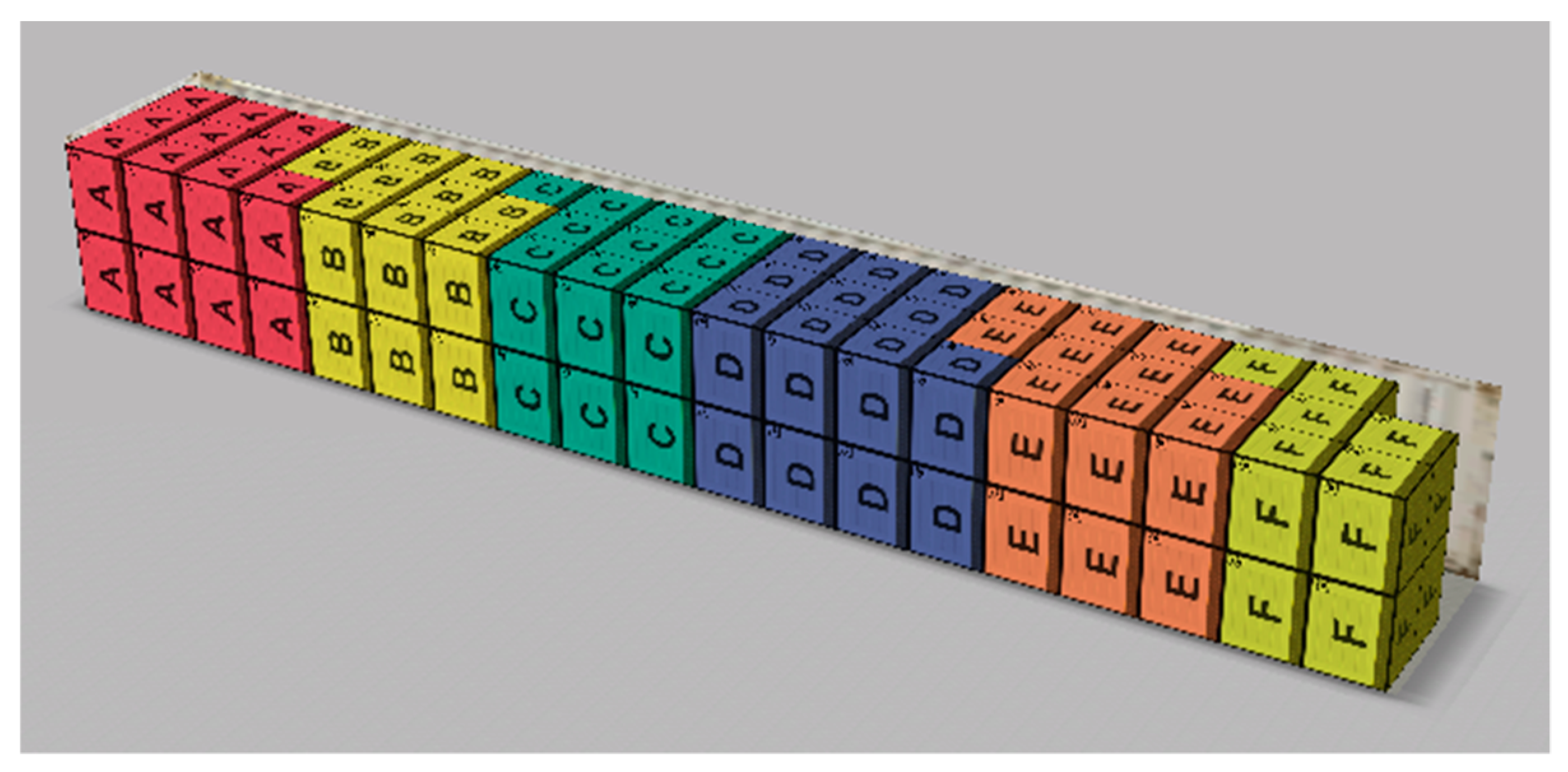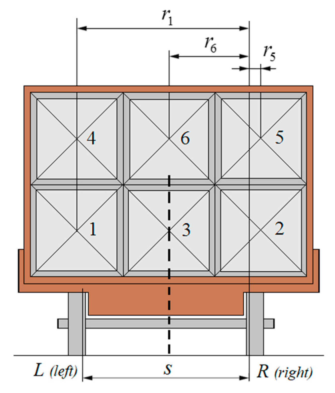Figure 3 shows the loading scheme of a Habis railcar, while the railcar’s characteristics are shown in Figure 6. One can see that the railcar’s carrying capacity depends on the railway line category (A, B or C).

The implemented RailLoad software was tested on a large number of examples in which pallets (manufactured after 2011) were loaded into single or multiple Habis railcars. The selected examples are described in Section 6.1 and Section 6.2. The initial assumption was that any type of cargo could be placed in any position. Depending on the example, additional requirements that have to be met will be defined. Also, we will consider that box pallets are homogeneous bodies i.e., that their center of gravity is in the volume center of gravity. The goods are going to be transported by means of C railway line category, where the max allowed one-axle weight is 20t and the max allowed weight by meter is 6.4t/m, when the standard track width is 1.435m. In view of the fact that pallets can be loaded onto each other, they can be loaded into the Habis wagon in two levels, namely 14 pallets can be placed lengthways and three pallets width ways. The wagon’s total volume capacity, in the number of pallets, is 84. All examples are tested in a running environment with Intel Core i5-6400 CPU 3.30GHz and 8 GB RAM. Freight railcar load planning is not time critical, and most often it can be done even days before starting the loading itself. Our goal was not to find the optimal solution for one, but the “good enough” solution for more optimization criteria, and to eliminate incorrect loading and securing of goods. Having this in mind, CPLEX Optimizer CPU execution time was limited to 600 seconds [s] for all examples, but some simpler examples are resolved to optimality in a much shorter period.

The examples below solve the task of how to optimize the packing of maximally 10 different PTs in railcars.

Table 2. A loading task involving 10 box PTs.

	PT1	PT2	PT3	PT4	PT5	PT6	PT7	PT8	PT9	PT10
net weight of the goods [kg]	780	310	480	490	410	490	530	630	780	830
profit	100	65	90	100	120	100	280	330	350	200
loading priority coefficient	1	1.1	1.2	1	1	1.3	1	1	1.2	1.1

shows the weight of each PT to be loaded, the profit made from transportation and the loading priority coefficient for each PT. In each example, the following three optimization criteria were observed: maximization of wagon load weight, maximization of wagon volume utilization and maximization of weighted profit, including loading priority coefficients.

6.1. Single Loading Examples

Example 1. 

Fifty pallets of each PTi, i = {1, …, 10} are available for loading. Only one type of goods should be loaded into wagon A.

The following cargo-related constraint that depends on the number of items due to be loaded PTi, i = {1, …, 10} is now included in the model:

$${\displaystyle \sum _{i=1}^m{\displaystyle \sum _{j=1}^n{x}_{ij}}}\le 50,\mathrm{for}\forall i\in \{1,\dots ,10\}.$$

(11)

The following separation constraint allows the loading of only one PT into a railcar:

$${\displaystyle \sum _{j=1}^n{\displaystyle \sum _{i=1}^m{x}_{ij}={\displaystyle \sum _{j=1}^n{x}_{kj}}}},\mathrm{for}\mathrm{some}k\in \{1,\dots ,10\}.$$

(12)

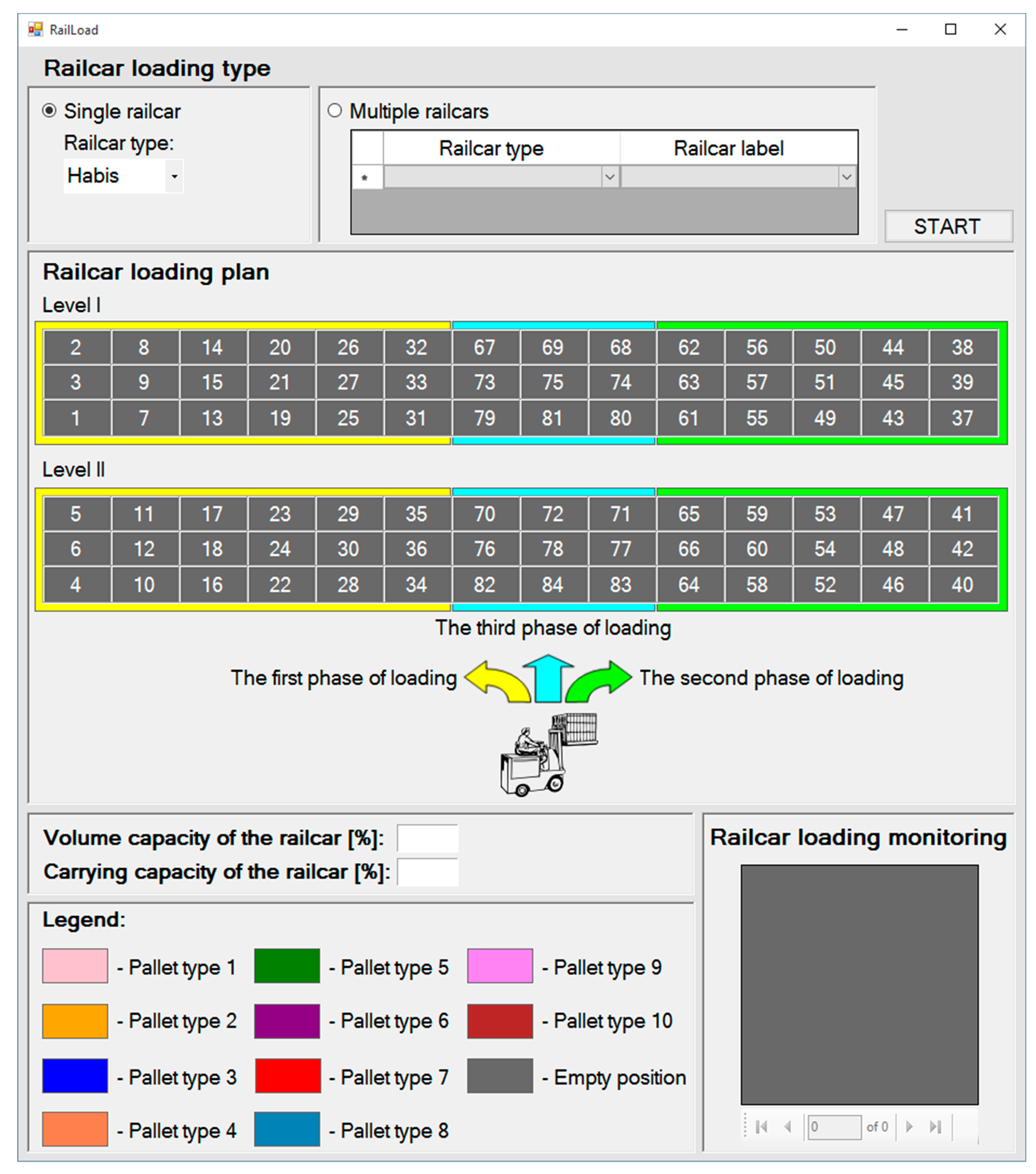
This is an example of the CLP classified as the IIPP. In the RailLoad application start window, the user selects option single railcar, railcar type: Habis, and activates the loading plan optimization software. The visualization of the achieved pallet arrangement generated by the RailLoad software is shown in Figure 7. In view of the objective function and the mathematical model described in Section 5.2, the loading of 50 PT7 pallets has been selected. We can see that, if a position on level I is empty, the corresponding position on level II has to be empty, too (e.g. 27 and 30, 63 and 66), while this, of course, is not the rule in the opposite case (e.g. positions 25 and 28, 26 and 29). The last position to be loaded is position 60. Thanks to the railcar loading monitoring panel, it is clear to the load organizer that there is a series of empty positions behind position 26.

Example 2. 

Fifty pallets of each Pti, i = {1, …, 10} are available for loading. They are to be loaded into wagon A.

The constraint (11) remains in force in this example as well. This problem is classified as a SLOPP: different PTs can be loaded into one wagon, so that the user selects the same options in the RailLoad application window as in the previous example. The software has generated a window with the problem solution, which will be left out here to save space. The solution details are outlined in

Table 3. The number of pallets by PT in the solution of Example 2.

	PT1	PT2	PT3	PT4	PT5	PT6	PT7	PT8	PT9	PT10
wagon A	0	4	0	0	0	0	50	24	6	0

and

Table 4. Wagon capacity utilization rate in Example 2.

Wagon	Total Load Weight [t]	Carrying Capacity [%]	Total Number of Pallets	Volume Utilization [%]	Weighted Profit	Real Profit
A	53.42	99.85	84	100	24,726	24,280

. The wagon can be filled to its volume capacity with the adequate number of four different PTs (PT2, PT7, PT8 and PT9), with a carrying capacity utilization rate of 99.85%.

6.2. Multiple Loading Examples

Example 3. 

Twenty pallets of each PTi, i = {1, 2, 3} due to be loaded have to be loaded by all means and they all have to be loaded into the same wagon. Also, 30 pallets of each PTi, i = {4, …, 10} are due to be loaded as well. There are two wagons, A and B, into which they can be loaded.

We are faced here, and in the examples below, with a problem classified as the MILOPP: different PTs have to be loaded into identical wagons. It is evident that the basic mathematical model described in Section 5.2 has to be modified taking into account the fact that the loading of items into two wagons is considered simultaneously. In this context, decision variables are as follows:

$$x_{ijR}=\{\begin{array}{l}1,\mathrm{if}\mathrm{a}\mathrm{PT}i\mathrm{is}\mathrm{assigned}\mathrm{to}\mathrm{position}j\begin{array}{c}\mathrm{in}\mathrm{railcar}\mathrm{R}\end{array}\\ 0,\mathrm{otherwise}\end{array},$$

(13)

where $x_{ijR}$ are 0–1 decision variables, i = {1, …, m}, j = {1, …, n}, R∈{A, B}.

Adapting other constraints to the loading of items into two wagons is not hard and will be left out here. Also, we have to introduce two additional constraints. Since items are to be loaded into two identical wagons (A and B), we can assume that the wagon into which all PTi, i = {1, 2, 3} will be loaded is wagon A. We therefore introduce the following connectivity constraint:

$${\displaystyle \sum _{j=1}^n{x}_{ijA}}=20,\mathrm{for}\forall i\in \{1,2,3\}.$$

(14)

Also, the following cargo-related constraint depends on the number of pallets due to be loaded PTi, i = {4, …, 10}:

$${\displaystyle \sum _{R\in \{A,B\}}^{}{\displaystyle \sum _{j=1}^n{x}_{ijR}}}\le 30,\mathrm{for}\forall i\in \{4,\dots ,10\}.$$

(15)

The RailLoad software has generated the solution, the details of which are outlined in

Table 5. The number of pallets by PT in the solution of Example 3.

	PT1	PT2	PT3	PT4	PT5	PT6	PT7	PT8	PT9	PT10
wagon A	20	20	20	0	0	0	9	2	13	0
wagon B	0	0	0	0	23	0	21	28	12	0

, visualizing it in a user-friendly user interface. Each wagon can be filled to its volume capacity with 84 pallets, with the wagon A carrying capacity utilization rate amounting to 99.91% and the wagon B carrying capacity utilization rate amounting to 99.89%. Twenty pallets of each PT including PT1, PT2 and PT3 are in wagon A, as specified by the constraint (14). Also, 9 PT7, 2 PT8 and 13 PT9 pallets are in the same wagon. The loading included seven different PTs, five of which (PT1, PT2, PT3, PT7 and PT8) have been fully loaded.

Example 4. 

Forty pallets of PT1, have to be loaded into wagon A. Thirty pallets of each PTi, i = {2, …,10} are due to be loaded. They can be loaded into two wagons, A and B. In total, 50 PT5 and PT8 pallets have to be loaded.

The constraint that all 40 PT1 pallets must be placed in wagon A is the following positioning constraint:

$${\displaystyle \sum _{j=1}^n{x}_{1jA}}=40.$$

(16)

The constraint (15) is valid in this example for ∀i∈{2, …, 10}. Also, we introduce a special constraint defining the total number of PT5 and PT8 pallets to be loaded:

$${\displaystyle \sum _{R\in \{A,B\}}^{}({\displaystyle \sum _{j=1}^n{x}_{5jR}}}+{\displaystyle \sum _{j=1}^n{x}_{8jR}})=50.$$

(17)

The RailLoad software has generated the solution, the details of which are outlined in

Table 6. The number of pallets by PT in the solution of Example 4.

	PT1	PT2	PT3	PT4	PT5	PT6	PT7	PT8	PT9	PT10
wagon A	40	30	0	0	3	0	11	0	0	0
wagon B	0	0	0	0	24	3	19	23	15	0

, visualizing it in a user-friendly user interface. Each wagon can be filled to its volume capacity with 84 pallets, with the wagon A carrying capacity utilization rate amounting to 99.89% and the wagon B carrying capacity utilization rate amounting to 99.91%. All 40 PT1 pallets are in wagon A, as specified by the constraint (16). The requirement (17) that 50 PT5 and PT8 pallets precisely have to be loaded has been met as well (three PT5 pallets are in wagon A, while 24 PT5 and 23 PT8 pallets are in wagon B). Of the available 10 PTs, the loading included seven different PTs, three of which (PT1, PT2 and PT7) have been fully loaded.

Example 5. 

Thirty pallets of each PTi, i = {1, …, 10}, are available for loading. They are to be loaded into three railcars: A, B, and C. The PT6 and PT7 items must not be placed in the same wagon.

Considering that three railcars are to be loaded, with the modification of the mathematical model described in Section 5.2 decision variables are now as follows:

$$x_{ijR}=\{\begin{array}{l}1,\mathrm{if}\mathrm{a}\mathrm{PT}i\mathrm{is}\mathrm{assigned}\mathrm{to}\mathrm{position}j\begin{array}{c}\mathrm{in}\mathrm{railcar}\mathrm{R}\end{array}\\ 0,\mathrm{otherwise}\end{array},$$

(18)

where $x_{ijR}$ are 0–1 decision variables, i = {1, …, m}, j={1, …, n}, R∈{A, B, C}.

The cargo-related constraint refers to the total number of pallets of each PTi available for loading:

$${\displaystyle \sum _{R\in \{A,B,C\}}^{}{\displaystyle \sum _{j=1}^n{x}_{ijR}}}\le 30,\mathrm{for}\forall i\in \{1,\dots ,10\}.$$

(19)

The separation constraint specifies that, if there is just one PT6 pallet in railcar A, B or C, no PT7 pallet can be placed in that railcar, and vice versa.

$$({\displaystyle \sum _{j=1}^n{x}_{6jR}}\ge 0\Rightarrow {\displaystyle \sum _{j=1}^n{x}_{7jR}}=0)\wedge ({\displaystyle \sum _{j=1}^n{x}_{7jR}}\ge 0\Rightarrow {\displaystyle \sum _{j=1}^n{x}_{6jR}}=0),\mathrm{for}\forall R\in \{A,B,C\}$$

(20)

Once the user has selected the loading into multiple railcars (option: Multiple railcars) in the RailLoad application start window, and Railcar type for each (Habis) railcar, the loading plan optimization software is activated. It first displays the loading plan for the railcar with label A, but the user can also select the tab showing the loading plan for a railcar with a different label, e.g. label B as shown in Figure 8.

Analyzing the loading plan for railcar B, we have concluded that the railcar can be filled to its volume capacity with 27 PT5 pallets, 29 PT6 pallets, 19 PT9 and 9 PT10 pallets. Also, the load organizer can clearly see the order in which a forklift truck should load the cargo: PT6, PT6, PT5, …, PT9, PT5, PT9.The railcar loading monitoring panel enables efficient monitoring of pallet loading. For example, if a forklift truck has just placed a PT5 pallet in position 3, it can be clearly seen that the next pallet to be placed in position 4 is also a PT5 pallet. The loading plan details for all three railcars are outlined in

Table 7. Capacity utilization rate per railcar in Example 5.

Wagon	Total Load Weight [t]	Carrying Capacity [%]	Total Number of Pallets	Volume Utilization [%]	Weighted Profit	Real Profit
A	53.49	99.98	84	100	23,946.5	23,105
B	54.45	99.91	84	100	16,970.0	14,590
C	53.44	99.89	84	100	11,153.0	10,150

and

Table 8. The number of pallets by PT in the solution of Example 5.

	PT1	PT2	PT3	PT4	PT5	PT6	PT7	PT8	PT9	PT10
wagon A	0	11	0	0	2	0	30	30	11	0
wagon B	0	0	0	0	27	29	0	0	19	9
wagon C	0	2	30	29	1	1	0	0	0	21

. PT6 pallets are in railcars B (29) and C (1), while all available PT7 pallets (30) are in railcar A, so that the constraint (19) has been fulfilled. Of the available 10 PTs, the loading included nine different PTs, seven of which (PT3, PT5, PT6, PT7, PT8, PT9 and PT10), i.e., all 30 available pallets, have been fully loaded.

Although there is a large number of papers dealing with CLP, we did not find academic publications that dealt specifically with loading to covered railcars, including real-world constraints tested on realistic benchmark data sets. We are sorry that we did not validate our solution in this way, however we strongly believe that the making of realistic benchmark data sets for this problem represents a challenge for future research. The software was validated by three experts for freight railcar loading by the following criteria:

• user-friendliness
• the speed of generating the solution
• correctness of the proposed loading plan
• clarity of graphical representation of the proposed loading plan
• reliability, i.e., the possibility to completely rely on loading plan generated by the RailLoad software
• clarity of load monitoring process.

Average rating by all criteria (in a range of 1 to 5, the higher the better) is 4.6.

7. Discussion and Conclusions

The brief analysis made in this paper has shown that incorrect loading is the dominant reason why freight railcars are withdrawn from service in the Republic of Serbia. In addition to jeopardizing safety, incorrect loading can result in cargo loss, damage or delivery delays, as well as damage to railway infrastructure and vehicles. It is clear that incorrect loading often generates unforeseen expenses (e.g. carriers’ expenses associated with payers of transportation services and vice versa, goods owners’ expenses associated with railcar owners and vice versa). The available loading software is insufficiently used for various reasons including the following: there are numerous exceptions to general loading rules which load planning users cannot include without the original code, loading plans are displayed in a non-standard form, or there are barriers in input/output communication between the loading software and the data store or the loading software and the user. Commercial software usually does not make it possible to monitor loading, especially sequential goods loading with a forklift truck. A change in the loading order of just two pallets if there is a significant difference in their weight can disrupt some important constraints affecting safety, e.g. the balance constraint.

Assuming that covered railcars are used as containers, this paper models and solves the loading of box pallets into railcars as a CLP-type C&P problem. As the loaded box pallets are of the same size and volume, although they can differ in gross weight, we can consider them a weakly heterogeneous set of cargo. The loading into a single railcar (CLP classified as the IIPP and SLOPP) as well as multiple identical railcars (CLP classified as the MILOPP) was observed. At the start, the basic mathematical model including standard orientation, complexity, positioning, weight, balance and stability constraints was formulated. Additional constraints were included in the models when necessary. The mathematical model was coded using the OPL and then solved with the help of CPLEX Optimizer, a mathematical programming solver. The generated solution of the mathematical model, the achieved loading plan, the solver stores in an Access database. The Windows application RailLoad, implemented in Visual Basic, communicates with the Access database and visualizes the loading plan, enabling its user-friendly monitoring. The software was tested in line with all standard criteria, while special attention was paid to its optimization and visualization features. The implemented software was tested on a large number of examples and it achieved “good enough” solutions for real-world usage regarding all observed optimization criteria: maximization of wagon load weight, maximization of wagon volume utilization and maximization of weighted profit. It can be concluded that the RailLoad software can offer full support to real planning problems and in particular to the clear monitoring of goods loading with a forklift truck.

The waysfor further research are numerous and make it necessary to extend both the model as well as the right software. Consequently, studying the loading of items into multiple heterogeneous railcars (a CLP classified as the MHLOPP) is one of the directions that maybe followed. Another direction could be analyzing how to load/unload at intermediate stations so as not to violate mandatory constraints at any point in time. Future researches must go towards the development of models that include all real-world constraints that will concern the loading of freight railcars [44]. This will increase the probability of their application in practice, but also give the possibility to evaluate and compare different solutions by using realistic benchmark data sets. Zhao et al. [16] emphasizes that “realistic and challenging data sets with clear real-world constraints would help move this research area forward.”