Elements of Hyperstructure Theory in UWSN Design and Data Aggregation

Abstract

In our paper we discuss how elements of algebraic hyperstructure theory can be used in the context of underwater wireless sensor networks (UWSN). We present a mathematical model which makes use of the fact that when deploying nodes or operating the network we, from the mathematical point of view, regard an operation (or a hyperoperation) and a binary relation. In this part of the paper we relate our context to already existing topics of the algebraic hyperstructure theory such as quasi-order hypergroups, $EL$-hyperstructures, or ordered hyperstructures. Furthermore, we make use of the theory of quasi-automata (or rather, semiautomata) to relate the process of UWSN data aggregation to the existing algebraic theory of quasi-automata and their hyperstructure generalization. We show that the process of data aggregation can be seen as an automaton, or rather its hyperstructure generalization, with states representing stages of the data aggregation process of cluster protocols and describing available/used memory capacity of the network.

1. Introduction

Underwater wireless sensor networks (UWSN) are often used in environment monitoring where they review how human activities affect marine ecosystems, undersea explorations such as detecting oilfields, for disaster prevention, e.g., when monitoring ocean currents, in assisted navigation for the location of dangerous rocks in shallow waters, or for disturbed tactical surveillance for intrusion detection.

The fact that such wireless sensor networks are deployed underwater results in profound differences from terrestrial wireless sensor networks. The key aspects that are different include the communication method, i.e., radio waves vs. acoustic signals, cost (while terrestrial networks experience decreasing prices of components, underwater sensors are still expensive devices), memory capacity (because water is a problematic medium resulting in the loss of large quantities of data), power limitations due to the nature of the signal and longer distances handled, as well as problems related to the deployment of the network, i.e., issues connected to static or dynamic deployment. In underwater sensor networks, we commonly face challenges of limited bandwith, high bit error rates, large propagation delays, and limited battery resources caused by the fact that in an underwater environment, sensor batteries are impossible to recharge especially because no solar energy is available underwater. The power losses, which cannot be avoided, result in the need to reconfigure the network topology in order to maintain network connectivity and communication between sensor nodes. Thus, size of the UWSN coverage area and efficiency of data aggregation are affected. Obviously, efficiency in battery use influences network lifetime without sacrificing system performances. These differences are shown in

Table 1. Comparison of some features of terrestrial and underwater wireless sensor networks (UWSN).

	(Terrestrial) WSN	UWSN
Communication Media	RF Waves	Acoustic Waves
Frequency	High	Low
Node size	Small	Large
Deployment	Dense	Sparse
Power	Low	High
Energy consumption	Low	High
Propagation delay	Low	High
Bandwidth	High	Low
Path loss	Low	High
Cost	Inexpensive	Expensive
Memory	Sensor nodes have low capacity	Sensor nodes require large capacity

.

We use different protocols for discovering and maintaining routes between sensor nodes. As mentioned in Novák, Křehlík, and Ovaliadis [1], the most commonly used routing protocols are: Flooding, multipath, cluster, and miscellaneous protocols, see Wahid and Dongkyun [2]. In the flooding approach, the transmitters send a packet to all nodes within the transmission range. In the multipath approach, source sensor nodes establish more than one path towards sink nodes on the surface. Finally, in the clustering approach the sensor nodes are grouped together in a cluster. For an easy-to-follow reading on how UWSN’s work and on advantages of clustering see Domingo and Prior [3], the basic idea is shown in Figure 1 and Figure 2.

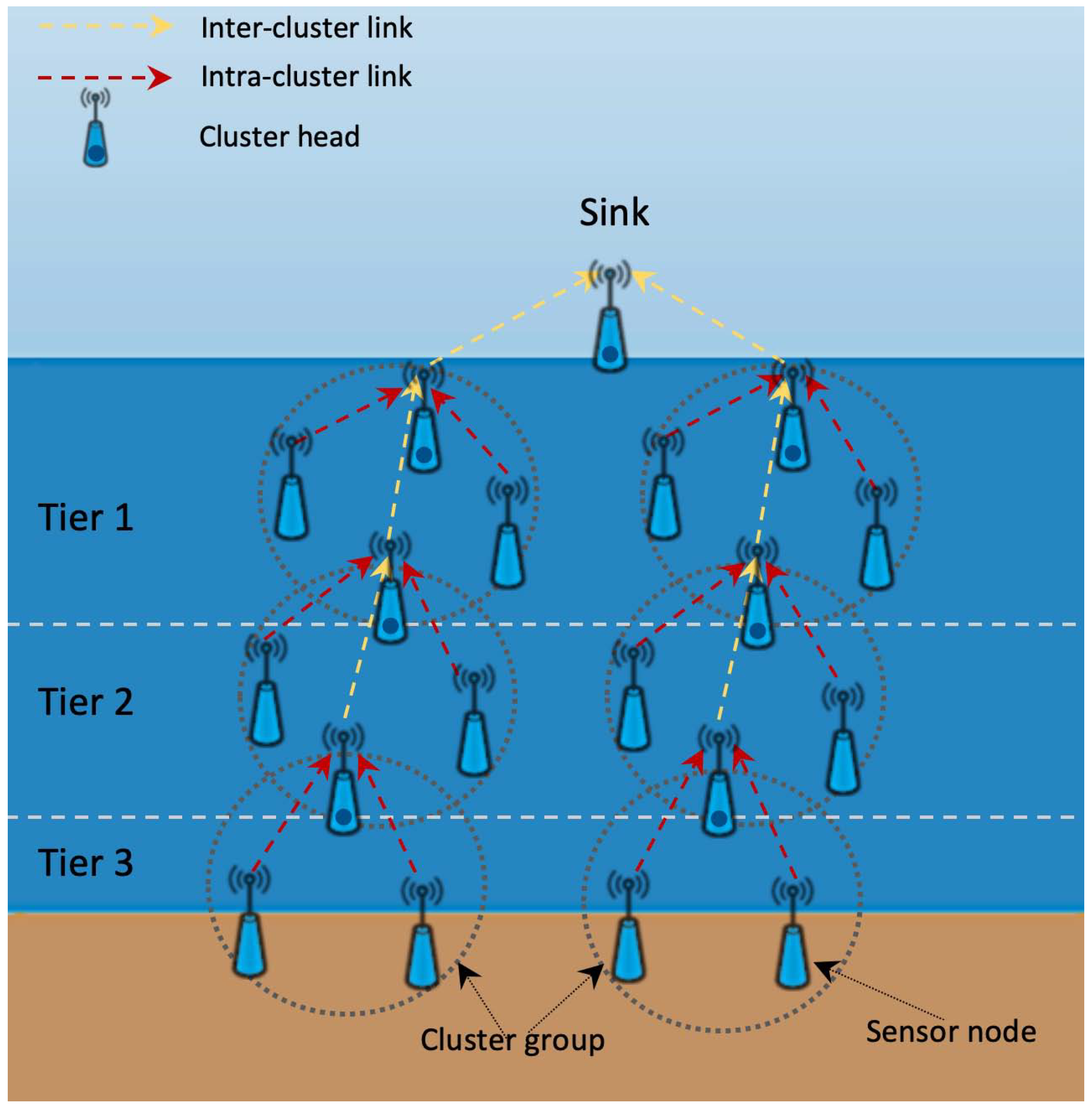
Recent research shows that the cluster based protocols give a great contribution towards the concept of energy efficient networks, see Ayaz et al. [4], Ovaliadis and Savage [5], or Rault, Abdelmadjid, and Yacine [6]. A common cluster based network consists of a centralized station deployed at the surface of the sea called a sink (or surface station) and sensor nodes deployed at various tiers inside the sea environment. These are grouped into clusters. In this architecture, each cluster has a head sensor node called a cluster head ($CH$). The cluster head is assumed to be inside the transmission range of all sensor nodes that belong to its cluster. Every cluster head operates as a coordinator for its cluster, performing significant tasks such as cluster maintenance, transmission arrangements, data aggregation, and data routing (Figure 2).

Mathematical Background of the Model

In the UWSN topology, several aspects are important for successful data aggregation. First of all, there must exist a path linking every element of the network to the surface station. However, these paths need not be unique as there might be multiple possible paths which the data from a given element can use to reach the surface station. Second, there always exists a cetain kind of ordering of the set of the network elements. They can be ordered with respect to their physical depth, with respect to their importance, with respect to communication priority, remaining battery power, etc. Finally, as data are collected, they are combined in the "upwards" elements in order to be sent further on.

Thus one may employ techniques of algebra or graph theory in the description of the data aggregation process as has been recently done by Aboyamita et al., Domingo, or Jiang et al. [7,8,9]. However, given the multivalued nature of data aggregation (multiple paths, more than one possible links of elements, etc.), it seems relevant to make use of the elements of the algebraic hyperstructure theory. Notice that while in "classical" algebra, we regard operations, i.e., mappings $f:H^n\to H$, in the algebraic hyperstructure theory we work with hyperoperations, i.e., mappings $g:H^n\to {\mathcal{P}}^{\ast }\left(H\right)$, where ${\mathcal{P}}^{\ast }\left(H\right)$ is the power set of H with ∅ excluded (one need not consider this exclusion though). For the general introduction to the theory as well as definitions of concepts not explicitly defined further on, see Corsini and Leoreanu [10].

In the algebraic hyperstructure theory, there are several concepts which make use of the aspect of ordering. A small selection includes Comer, Corsini, Cristea, De Salvo et al. [11,12,13,14,15]. Further on we discuss three of these: $EL$–hyperstructures, quasi-order hypergroups, and ordered hyperstructures. Each of these concepts uses somewhat different background and assumptions:

• $EL$–hyperstructures are constructed from pre- and partially-ordered semigroups, i.e., the hyperoperation is defined using an operation and a relation compatible with it;
• Quasi-order hypergroups are constructed from pre-ordered sets, i.e., the hyperoperation is defined using a relation only;
• Ordered hyperstructures are algebraic hyperstructures on which a relation compatible with the hyperoperation is defined.

All of these have been studied in depth and numerous results have been achieved in their respective theories. The idea of $EL$–hyperstructures has been implicitely present in a number of works since at least the 1960s, for example Pickett [16]. The definition and first results were given by Chvalina [17] and the theory has been elaborated by Novák (later jointly with Chvalina, Křehlík, and Cristea) in a series of papers including [18,19,20,21,22]. It is to be noted that, since the class of $EL$–hyperstructures is rather broad, the aim of many theorems included in some of those papers was to establish a common ground for some already existing ad hoc derived results. Recently, some examples concerning various types of cyclicity in hypergroups have been constructed using $EL$–hyperstructures, see Novák, Křehlík and Cristea [23].

The idea of quasi-order hypergroups was proposed by Chvalina in [17,24,25]. Some results achieved with the help of this concept are included in Corsini and Leoreanu [10]. Not to be missed are results concerning the theory of automata collected in Chvalina and Chvalinová [25]. It should be stressed that these results were motivated by Comer [26] and Massouros and Mittas [27].

Ordered hyperstructures were introduced by Heidari and Davvaz [28]. Numerous results have been published since, mainly by Iranian authors.

For the following set of basic definitions see Novák, Křehlík, and Ovaliadis [1].

Definition 1.

By an $EL$–semihypergroup we mean a semihypergroup, in which, for all $a,b\in H$, there is $a\ast b=\{x\in H\mid a·b\le x\}$, where $(H,·,\le )$ is a quasi-ordered semigroup.

Proposition 1.

[20,22] If, for all $a,b\in H$, there is $\{a,b\}\in a\ast b$, then the $EL$–semihypergroup $(H,\ast )$ is a hypergroup. If $(H,·,\le )$ is a partially ordered group, then its $EL$–hypergroup $(H,\ast )$ is a join space.

Definition 2.

Let $(H,\ast )$ be a hypergroupoid. We say that H is a quasi-order hypergroup, i.e., a hypergroup determined by a quasi-order, if, for all $a,b\in H$, $a\in a^3=a^2$, and $a\ast b=a^2\cup b^2$. Moreover, if $a^2=b^2\Rightarrow a=b$ holds for all $a,b\in H$, then $(H,\ast )$ is called an order hypergroup.

Proposition 2.

[10] A hypergroupoid is a quasi-order hypergroup if and only if there exists a quasi-order "≤" on the set H such that, for all $a,b\in H$, there is $a\ast b={\left[a\right)}_{\le }\cup {\left[b\right)}_{\le }.$

Definition 3.

An ordered semihypergroup $(H,\ast ,⪯)$ is a semihypergroup $(H,\ast )$ together with a partial ordering "⪯" which is compatible with the hyperoperation, i.e., $x⪯y\Rightarrow a\ast x⪯a\ast y\mathrm{and}x\ast a⪯y\ast a$ for all $a,x,y\in H$. By $a\ast x⪯a\ast y$ we mean that for every $c\in a\ast x$ there exists $d\in a\ast y$ such that $c⪯d$.

Notation. Further on, for some $a\in H$, by ${\left[a\right)}_{\le }$ means the set $\{x\in H\mid a\le x\}$. For this reason, closed intervals will not be denoted by $[a,b]$ but by $\langle a;b\rangle$.

2. Mathematical Model

The mathematical model presented in this section was published as an extended abstract of the conference contribution Novák, Ovaliadis, and Křehlík [1] presented by the authors of this paper at International Conference on Numerical Analysis and Applied Mathematics (ICNAAM 2017).

UWSNs consist of elements of different types: First, we have surface stations, which pass data to a ship or to a data-collecting station located on the sea shore; second, we have sensor nodes deployed at various tiers in water or at the sea bed. The sensors, which are deployed in water, can function as sensors measuring the requested data or as transporters of information from seabed sensors. In any case, information collected from all sensors must be passed to surface stations. From these it can be collected either by a ship passing by or, alternatively, transmitted to a data-collecting station located on the sea shore. The ship or the data-collecting stations are central nodes.

Denote H the set of all elements of an arbitrary UWSN. Suppose that all elements are capable of handling (i.e., receiving or transmitting) data in the same way. Also suppose that they perform the same set of tasks. Thus they are, from the mathematical point of view, interchangeable and equal (of course, with respect to their functionality as sinks and sensor nodes). The aim of the system is to collect information. 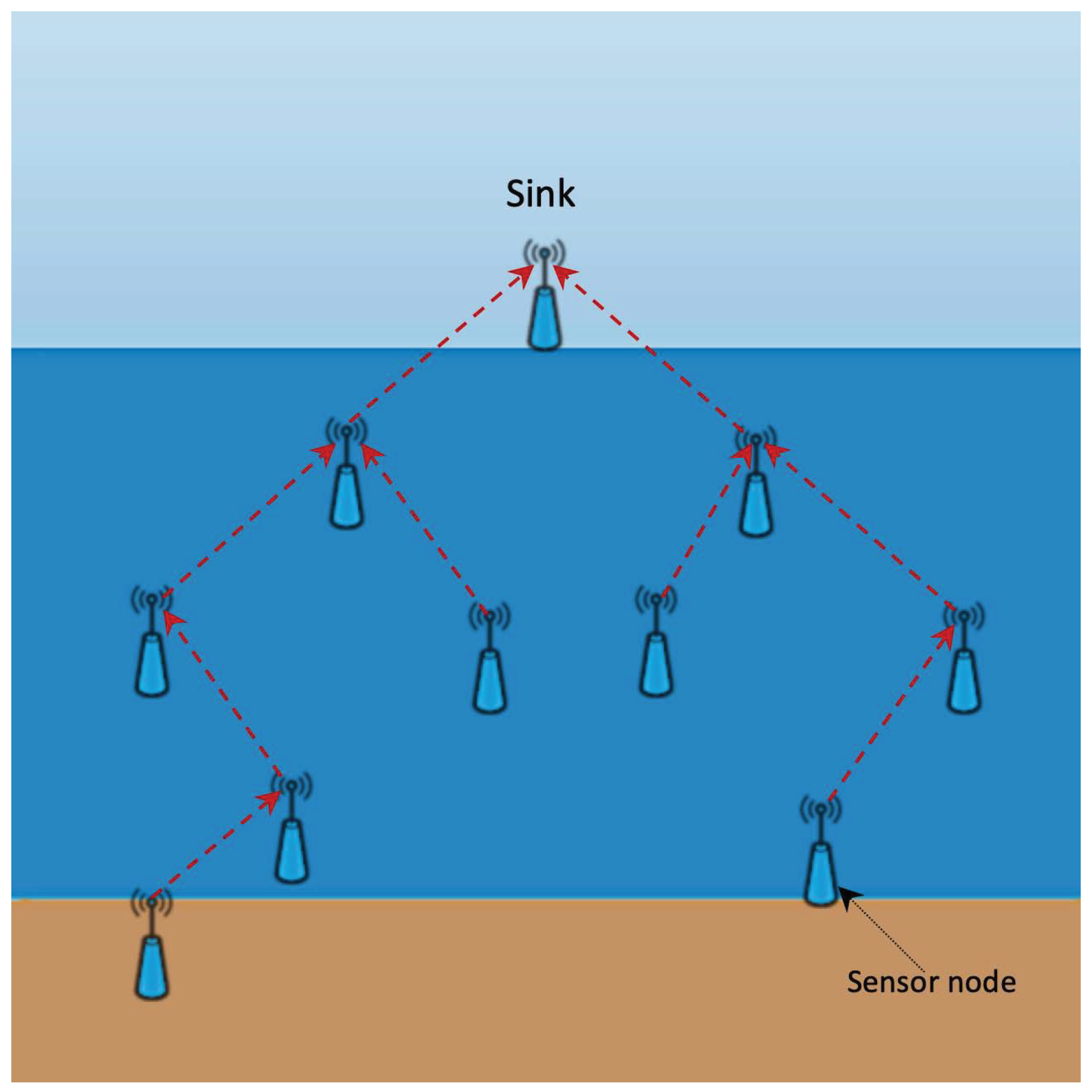Therefore, our elements of H must communicate data. This should be done ideally upwards, towards the surface. As we have mentioned above, there are different ways of passing information. In our model we concentrate on multipath and cluster routing approach (see Figure 1 and Figure 2). For details concerning these see Ayaz et al. and Li et al. [4,29]. Multipath routing protocols (Figure 1), forward the data packets to the sink via other nodes while in cluster based routing protocols (Figure 2), data packets are first aggregated to the respective cluster heads and only then forwarded via other cluster heads to the sink. For our purposes, we denote the i–th cluster by $c{l}_i$. Its cluster head will be denoted by $C{H}_i$. We call non-$CH$ nodes ordinary and sinks will be treated as cluster heads.

Now, suppose that the elements of our system are clustered. In other words, some elements of H function as cluster heads, i.e., masters, while others are ordinary. The data aggregation process goes as follows: Within their cluster, the ordinary elements pass information to their cluster head while between clusters, i.e., supposedly over longer distances, only cluster heads communicate. At a given point in time, each cluster has the unique cluster head, and each element can belong to exactly one cluster. We denote the i–th cluster by $c{l}_i$ and its cluster head by $C{H}_i$.

Now, for a given pair $a,b\in H$, regard a binary hyperoperation, where $a\ast b$ is, for arbitrary $a,b\in H$, defined by:

$$\begin{array}{c}\hfill a\ast b=\left\{\begin{array}{cc}\{a,b\}\cup {[a·b)}_{\le }\hfill & \mathrm{for}(a=C{H}_i,b=C{H}_j)\mathrm{or}a,b\in c{l}_i\hfill \\ \{a,b\}\hfill & \mathrm{for}(a\ne C{H}_i\mathrm{or}b\ne C{H}_j)\mathrm{and}(a\in c{l}_i,b\in c{l}_j,i\ne j)\hfill \end{array}\right.\end{array}$$

(1)

By ${[a·b)}_{\le }$ we mean a set $\{x\in H\mid a·b\le x\}$, where $a·b$ is a result of a single-valued binary operation such that $a·b$ is, for arbitrary $a,b\in H$, defined by:

$$\begin{array}{c}\hfill a·b=\left\{\begin{array}{cc}C{H}_i\hfill & \mathrm{for}a,b\in c{l}_i\hfill \\ C{H}_k\hfill & \mathrm{for}a=C{H}_i,b=C{H}_j,i\ne j\hfill \\ s\hfill & \mathrm{for}\left((a\ne C{H}_i\mathrm{or}b\ne C{H}_j)\mathrm{and}(a\in c{l}_i,b\in c{l}_j,i\ne j)\right)\mathrm{or}a=s\mathrm{or}b=s\hfill \end{array}\right.\end{array}$$

(2)

and $C{H}_k$ is such a cluster head that $C{H}_i\le C{H}_k$, $C{H}_j\le C{H}_k$, where $a\le b$ is a relation between elements of H such that: (1) $s\le s$, $s\le C{H}_i$ and $C{H}_i\le s$ for all clusters $c{l}_i$, (2) within the same cluster $c{l}_i$ we have $a_j\le C{H}_i$ for all $a_j\in c{l}_i$ while mutually different ordinary elements of the cluster are incomparable, (3) between clusters for $a=C{H}_i$, $b=C{H}_j$ the fact that $a\le b$ means that the tier of b (measured towards the surface) is smaller than or equal to the tier of a, and (4) in all other cases a and b are not related. By $C{H}_k$ above we mean a cluster head on the closest tier above both $C{H}_i$ and $C{H}_j$. Of course, $C{H}_k$ always exists yet need not be unique as there may be more cluster heads at this closest tier. In such a case, we choose the most suitable one or regard all cluster heads as equal. Notice that, in our definitions, the fact that $C{H}_i\le C{H}_j$ and simultaneously $C{H}_j\le C{H}_i$ does not mean that $C{H}_i=C{H}_j$, rather it only means that $C{H}_i$ and $C{H}_j$ are on the same tier. If we are able to chose the most suitable cluster head (further on we remark that we are), the relation "≤" (restricted to $H\backslash \left\{s\right\}$) becomes partial ordering and we can write $C{H}_k=sup\{C{H}_i,C{H}_j\}$ (with respect to the relation "≤"). Finally, the element s is an element of H reserved for situations when a and b fail to communicate. It is artificially added to our set of elements H or we can agree that one (given the actual sensor deployment is of course carefully chosen) of elements of H will be s. In this way, technically speaking, we should in fact write $H_e=H\cup \left\{s\right\}$, where $H_e$ could mean "expanded". Of course, if we choose the option of $s\in H$, then $H_e=H$.

Under these definitions, $a·b$ is the element in which the data from a and b meet, and $a\ast b$ is the path in which the data from both a and b can spread. The facts that $a·b=s$ or $a\ast b=\{a,b\}$ or $a\ast b=\{a,b,s\}$ all stand for communication failure.

Lemma 1.

[1] $(H,\le )$ is a quasi-ordered set.

Suppose now that we have arbitrary $a,b\in H$. Since the result of $a·b$ is such an element of H in which the data from a and b meet, it is natural to suppose that $a·b=b·a$, i.e., that "·" is commutative. However, we can suppose this only on condition that there exists such an algorithms that $a·b=C{H}_k=C{H}_l=b·a$ for arbitrary clusters $c{l}_k,c{l}_l$. Further on suppose that such an algorithm exists, i.e., that $(H,·)$ is a commutative groupoid. The following lemma is obvious.

Lemma 2.

[1] If $(H,·)$ is a commutative groupoid, then $(H,\ast )$ is a commutative hypergroupoid.

In the following lemma notice that weak associativity of the hyperoperation is defined as $a\ast (b\ast c)\cap (a\ast b)\ast c\ne \varnothing$ for all $a,b,c\in H$; a quasi-hypergroup is a reproductive hypergroupoid.

Lemma 3.

[1] The hypergroupoid $(H,\ast )$ is a $H_v$–group, i.e., a weak associative quasi-hypergroup.

Lemma 4.

[1] The quasi-ordering "≤" and the operation "·" are compatible, i.e., for all $a,b\in H$ such that $a\le b$ and an arbitrary $c\in H$ there is $a·c\le b·c$ and $c·a\le c·b$.

Now, denote $H_{CH}\subseteq H$ the set of cluster heads. This notation enables us to regard both clustering based systems and multipath systems because the fact that $H_{CH}=H$ means that every element of H is a cluster head, i.e., the system is in fact a multipath one. In such a case the model simplifies substantially. This is because there is no need for the special element s and we do not distinguish between communication within and between clusters. The operation "·" defined by Equation (2) reduces to $a·b=c$ (we still suppose that it is commutative) and, consequently, the hyperoperation Equation (1) reduces to $a\ast b=\{a,b\}\cup {[a·b)}_{\le }$, in both cases for all $a,b\in H$.

Lemma 5.

[1] If we are able to uniquely identify $C{H}_k$ in Equation (2), then $(H_{CH},·,\le )$ is a partially ordered semigroup.

Finally, what is $x\in {\left[a\right)}_{\le }$? This means that $a\le x$, i.e., that the data from the element a reach the element x. Thus, if x is a sink, than the fact that $x\in {\left[a\right)}_{\le }$ means that the data from a can be successfully collected. What we want is that, if we denote S the set of all sinks, for all $a\in H$ there exists at least one $x\in S$ such that $x\in {\left[a\right)}_{\le }$, which means that data from all elements of our network H can be successfully collected. Of course, in order to achieve this, it is crucial to have an algorithm for unique determination of $C{H}_k$ in Equation (2). Yet clustering algorithms such as the Distributed Underwater Clustering Scheme (DUCS) [3] or Low Energy Adaptive Clustering Hierarchy (LEACH) protocol can provide this.

3. Use of the Theory of Quasi-Automata

In Definition 2, the concept of quasi-order hypergroup is defined. Chvalina and Chvalinová [25] relate these to the theory of quasi-automata, i.e., automata without output. For an automaton they construct a quasi-order hypergroup of its state set and show that the automaton is connected if and only if the state hypergroup is inner irreducible as well as strogly connected, i.e., we can reach any state from any other state, if and only if the state hypergroup is (in a special way) cyclic. In other words, if we look at the problem of data aggregation from the point of view of the automata theory, where every step is an application of the transition function with the initial state "data aggregation to begin" and the desirable state "data from all elements collected" (or rather "useful data from all elements sent" since every $CH$ not only receives data but also separates useful data from useless ones), we should be interested in constructing such automata or studying their properties.

We call the concept defined below quasi-automaton even though this term is not much frequent (we do this to be consistent with some earlier papers on hyperstructure theory). In fact, we could speak of semiautomata or deterministic finite automata (the below mentioned paper Chvalina and Chvalinová [25] uses a general term automaton; however, notice that [25], p. 107, plain text, defines automaton in the way of Definition 4, which is a definition adopted by the authors of [25] in later years). For an overall discussion of the concepts and the reasons for our choice of the name see Novák et al. [30]. For some further reading and applications see also Hošková et al. [31,32,33].

Definition 4.

By a quasi–automaton we mean a structure $\mathbb{A}=(I,S,\delta )$ such that $I\ne \varnothing$ is a monoid, $S\ne \varnothing$ and $\delta :I\times S\to S$ satisfies the following condition:

1.

There exists an element $e\in I$ such that $\delta (e,s)=s$ for any state $s\in S$;

2.

$\delta (y,\delta (x,s\left)\right)=\delta (xy,s)$ for any pair $x,y\in I$ and any state $s\in S.$

The set I is called the input set or input alphabet, the set S is called the state set and the mapping δ is called next-state or transition function. Condition 2 is called GMAC (Generalized Mixed Associativity Condition).

In [25], Chvalina and Chvalinová defined what they called a state hypergroup of an automaton. This is in fact a state set with a special hyperoperation, defined by means of the transition function. In this way, the concept of a state hypergroup is fixed to the automata theory. However, the way of defining this concept is a parallel to the concept of quasi-order hypergroups, which means that state hypergroups of quasi-automata are quasi-order hypergroups. The fact that the below defined $(S,\circ )$ is a hypergroup, or rather quasi-order hypergroup, (hence the name state hypergroup) was proved in [25]. (Notice that in [25] I and S are swapped.)

Definition 5.

Let $\mathbb{A}=(I,S,\delta )$ be an automaton. We define a binary hyperoperation "∘" on the state set S by:

$$s\circ t=\delta (I^{*},s)\cup \delta (I^{*},t)$$

(3)

for any pair of states $s,t\in S$, where $A^{*}$ is a free monoid of words over the (non-empty) alphabet A. The hyperstructure $(S,\circ )$ is called state hypergroup of the automaton $\mathbb{A}$.

Some properties of automata following from properties of its state hypergroup are proved in [25]. This includes the properties of being connected or separated.

Definition 6.

Let $\mathbb{A}=(I,S,\delta )$ be a quasi-automaton. A quasi-automaton $\mathbb{B}=(I,S_1,{\delta }_1)$ such that $S_1\subseteq S$ and ${\delta }_1$ is a restriction of δ on $I\times S_1$ and $\delta (a,s)\in S_1$ for any state $s\in S_1$ and any word $a\in I^{*}$, is called a sub quasi-automaton of $\mathbb{A}$. A sub quasi-automaton $\mathbb{B}=(I,S_1,{\delta }_1)$ of a quasi-automaton $\mathbb{A}=(I,S,\delta )$ is called separated if $\delta (S\backslash S_1,I^{*})\cap S_1=\varnothing$. A quasi-automaton is called connected if it does not posses any separated proper subautomaton. A quasi-automaton $\mathbb{A}=(I,S,\delta )$ is called strongly connected if for any states $s,t\in S$ there exists a word $a\in I^{*}$ such that $\delta (a,s)=t$.

If in quasi–automata we suppose that the input set I is a semihypergroup instead of a free monoid, we arrive at the concept of a quasi–multiautomaton. When defining this concept, caution must be exercised when adjusting the conditions imposed on the transition function $\delta$ as on the left-hand side of condition 2 we get a state while on the right-hand side we get a set of states. However, in the dichotomy deterministic — nondeterministic, quasi–multiautomata still are deterministic because the range of $\delta$ is S. The difference between the transition function of a quasi-automaton and the transition function of a quasi-multiautomaton is that in quasi-automata the state achieved by applying y in a state, which is the result of application of x in s, is the same as the state achieved by applying $xy$ in s, while condition (4) says that it is one of the many states achievable by applying any command from $x\ast y$ in state s.

Definition 7.

A quasi–multiautomaton is a triad $\mathbb{A}=(I,S,\delta )$, where $(I,\ast )$ is a semihypergroup, S is a non–empty set, and $\delta :I\times S\to S$ is a transition map satisfying the condition:

$$\delta (b,\delta (a,s\left)\right)\in \delta (a\ast b,s)\mathit{for}\mathit{all}a,b\in I,s\in S.$$

(4)

The hyperstructure $(I,\ast )$ is called the input semihypergroup of the quasi–multiautomaton $\mathbb{A}$ (I alone is called the input set or input alphabet), the set S is called the state set of the quasi–multiautomaton $\mathbb{A}$, and δ is called next-state or transition function. Elements of the set S are called states, elements of the set I are called input symbols.

Further on, we will make use of the above mentioned concepts to model the process of data aggregation. Notice that in Novák et al. [30], Cartesian composition of automata resulting in a quasi-multiautomaton is used to describe a task from collective robotics. Moreover, in Chvalina et al. [18], the issue of state sets and input sets having the form of vectors and matrices (of both numbers and special classes of functions) is discussed in the context of quasi-multiautomata.

In Figure 2 we can see that the elements of the UWSN are divided into several tiers. Also, the nodes are grouped into clusters. The process of data aggregation happens as follows: First, data is collected in cluster heads and then transmitted between cluster heads towards the surface, i.e., "upwards". Obviously, we can only transmit the amount of data that the capacity of available memory allows. Suppose that clusters cover areas of more or less the same size, i.e., it does not matter how many nodes there are in respective clusters. Now, regard a set of vectors:

$$S_v=\{\overrightarrow{v}=(v_1,v_2,\dots ,v_n)\mid v_i\in \langle 0;1\rangle ;i\in \{1,\dots ,n\}\}$$

(5)

of such a number of components that corresponds to the number of tiers (with index 1 meaning surface and index n meaning seabed or the deepest tier). The components $v_i$ carry information about how much total memory all cluster heads at a given tier has been used. In other words, $v_2=0.6$ means that at the second tier $60\%$ memory capacity has been used, regardless of whether this $60\%$ means that every cluster head at this level has $40\%$ free capacity or whether 6 out of 10 cluster heads already have no available memory while 4 are $100\%$ free.

The process of data aggregation starts with $\overrightarrow{v}=(0,\dots ,0)$, i.e., at the moment when all cluster heads have empty memory. Since, at first data are collected within clusters, $\overrightarrow{v}$ immediately becomes non-zero. The process of communication between cluster heads is described by the change of $\overrightarrow{v}$ by means of multiplying $\overrightarrow{v}$ by a square matrix of real numbers:

$$I_M=\left\{{\mathbf{A}}_k=\left[\begin{array}{ccc}{a}_{11}& \cdots & a_{1n}\\ \cdots & \cdots & \cdots \\ a_{n1}& \cdots & a_{nn}\end{array}\right]\mid a_{ij}\in \langle 0;1\rangle \mathrm{for}i\ge j,a_{ij}=0\mathrm{for}i<j;i,j\in \{1,\dots ,n\};{\parallel {\mathbf{A}}_k\parallel }_1\le 1\right\},$$

where $\parallel {\mathbf{A}}_k{\parallel }_1$ is the column norm of ${\mathbf{A}}_k$. In other words, $I_M$ is a subset of the set of upper triangular matrices, i.e., we can also write:

$$I_M=\left\{{\mathbf{A}}_k=\left[\begin{array}{ccccc}{a}_{11}& 0& 0& \cdots & 0\\ a_{21}& a_{22}& 0& \cdots & 0\\ ⋮& ⋮& \ddots & ⋮& ⋮\\ a_{n1}& a_{n2}& a_{n3}& \cdots & a_{nn}\end{array}\right]\mid {\parallel {\mathbf{A}}_k\parallel }_1\le 1\right\}$$

(6)

Now, these two sets $S_v$ and $I_M$ will be linked with a transition function $\delta$ by:

$$\delta (\mathbf{A},\overrightarrow{v})=\overrightarrow{v}·\mathbf{A}$$

(7)

for all $\mathbf{A}\in I_M$ and all $\overrightarrow{v}\in S_v$. If we regard the usual matrix multiplication (only swapped), i.e., $\mathbf{A}\odot \mathbf{B}=\mathbf{B}·\mathbf{A}$ for all $\mathbf{A},\mathbf{B}\in I_M$, then $(I_M,\odot )$ is a monoid such that the free monoid $I_M^{*}=I_M$. Thus we can regard the triple $(I_M,S_v,\delta )$ and study whether it is a quasi-automaton. In our context, the operation of creating words from input symbols of our alphabet I will be matrix multiplication, i.e., a word will be a product of matrices, i.e., again a matrix.

Theorem 1.

The triple $(I_M,S_v,\delta )$ is a quasi-automaton.

Proof. 

The identity matrix $E_n$ is the neutral element of $I_M$. Property 1 of Definition 4 holds trivially. Verification of Property 2 is also straightforward:

$$\delta (\mathbf{A},\delta (\mathbf{B},\overrightarrow{v}))=\delta (\mathbf{A},\overrightarrow{v}·\mathbf{B})=(\overrightarrow{v}·\mathbf{B})·\mathbf{A}=\overrightarrow{v}·\mathbf{B}·\mathbf{A}=\delta (\mathbf{B}·\mathbf{A},\overrightarrow{v})=\delta (\mathbf{A}\odot \mathbf{B},\overrightarrow{v}).$$

 □

The set $I_M$ consists of matrices such that the column norm ${\left|\right|\mathbf{A}\left|\right|}_1$ is at most one. In the following Remark, we show that without this condition the set $I_M$ would not be closed with respect to "⊙".

Remark 1.

Suppose two matrices $\mathbf{A},\mathbf{B}\in I_M$. If we denote:

$$\mathbf{A}=\left[\begin{array}{ccccc}{a}_{11}& 0& 0& \cdots & 0\\ a_{21}& a_{22}& 0& \cdots & 0\\ ⋮& ⋮& \ddots & ⋮& ⋮\\ a_{n1}& a_{n2}& a_{n3}& \cdots & a_{nn}\end{array}\right]\mathbf{B}=\left[\begin{array}{ccccc}{b}_{11}& 0& 0& \cdots & 0\\ b_{21}& b_{22}& 0& \cdots & 0\\ ⋮& ⋮& \ddots & ⋮& ⋮\\ b_{n1}& b_{n2}& b_{n3}& \cdots & b_{nn}\end{array}\right],$$

then,

$$\mathbf{B}\odot \mathbf{A}=\mathbf{A}·\mathbf{B}=\left[\begin{array}{ccccc}{\displaystyle \sum _{i=1}^1}{a}_{1i}{b}_{i1}& 0& 0& \cdots & 0\\ {\displaystyle \sum _{i=1}^2}{a}_{2i}{b}_{i2}& {\displaystyle \sum _{i=2}^2}{a}_{2i}{b}_{i2}& 0& \cdots & 0\\ ⋮& ⋮& \ddots & ⋮& ⋮\\ {\displaystyle \sum _{i=1}^n}{a}_{ni}{b}_{in}& {\displaystyle \sum _{i=2}^n}{a}_{ni}{b}_{in}& {\displaystyle \sum _{i=3}^n}{a}_{ni}{b}_{in}& \cdots & {\displaystyle \sum _{i=n}^n}{a}_{ni}{b}_{in}\end{array}\right]$$

and it is obvious that the column norm ${\parallel \mathbf{B}\odot \mathbf{A}\parallel }_1$ will not exceed 1, i.e., $\mathbf{B}\odot \mathbf{A}\in I_M$. Indeed, suppose that $\mathbf{A}$ is an all-ones matrix upper triangular matrix (which, of course violates the condition that ${\parallel \mathbf{A}\parallel }_1\le 1$). Then all the sums in $\mathbf{B}\odot \mathbf{A}$ reduce to ${\displaystyle \sum _{i=j}^n}{b}_{ij}$ which are (due to the fact that ${\parallel \mathbf{B}\parallel }_1\le 1$) smaller than 1. If moreover ${\parallel \mathbf{A}\parallel }_1\le 1$, none of the sums becomes greater. Of course, in $I_M$ we could have used the row norm instead of column one with the same result.

Example 1.

Regard sensor nodes deployed under water, which are divided into four tiers with tier 1 being $0–25m$, tier 2 being $25–50m$, tier 3 being $50–75m$, and tier 4 being $75–100m$ under water. Every tier has an arbitrary number of clusters, i.e., an arbitrary number of cluster heads, each with the same memory capacity. Then by vector e.g., $\overrightarrow{v}=(0.3;0.1;0;0.5)$, we describe such a state of the system that, at a certain point in time, $30\%$ data has been collected (or rather, $30\%$ memory capacity has been used) from tier 1 with the numbers being $10\%$ from tier 2, $0\%$ from tier 3, and $50\%$ from tier 4. Now regard a matrix:

$$\mathbf{A}=\left[\begin{array}{cccc}0& 0& 0& 0\\ 1& 1& 0& 0\\ 0& 0& 0& 0\\ 0& 0& 1& 0\end{array}\right]\in I_M,$$

which we apply on $\overrightarrow{v}$. Then $\delta (\mathbf{A},\overrightarrow{v})=(0.1;0.1;0.5;0)$, which describes the new state of the system. Of course, the first $30\%$ of data (represented by the first component of $\overrightarrow{v}$) did not get lost, which we can regard as output, i.e., to each quasi-automaton we can assign output, meaning that data from the upmost tier 1 have been processed, sent out of the system. Furthermore, in our example, data from tier 2 were transferred to tier 1 (and left in tier 2, i.e., in this case we have a backup copy). Also, data from tier 4 were transferred to tier 3, which had been empty, and simultaneously deleted in tier 4. It can be easily observed that the issue of suitable construction of matrices used for quasi-automata inputs is a topic for further research which will be closely linked to various aspects of optimization theory.

When describing the state hypergroup of $(I_M,S_v,\delta )$, we must first of all decide whether or not $(S_v,\circ )$ defined by Equation (3) is trivial. However, this task is rather simple.

Lemma 6.

The state hypergroup $(S_v,\circ )$ of $(I_M,S_v,\delta )$ is not trivial, i.e., there exist states $s,t\in S_v$ such that $\varnothing \ne \delta (I_M^{*},s)\cup \delta (I_M^{*},t)\ne S_v$.

Proof. 

The transition function $\delta$ is defined on $(I_M,S_v,\delta )$ by $\delta (\mathbf{A},\overrightarrow{v})=\overrightarrow{v}\mathbf{A}$ for all $\mathbf{A}\in I_M$ and all $\overrightarrow{v}\in S_v$. Moreover, by Equation (5), components of vectors from $S_v$ are real numbers from interval $\langle 0;1\rangle$, and by (6) matrices from $I_M$ are upper triangular with entries taken from the same interval. Finally, in a text preceding Theorem 1 we have already mentioned that $I_M^{*}=I_M$. Thus, for all $s,t\in I_M$ and all $\mathbf{A}\in I_M$, we have that:

$$\delta (\mathbf{A},\overrightarrow{s})=\overrightarrow{s}\mathbf{A}=(s_1,s_2,\dots ,s_n)\left[\begin{array}{ccccc}{a}_{11}& 0& 0& \cdots & 0\\ a_{21}& a_{22}& 0& \cdots & 0\\ ⋮& ⋮& \ddots & ⋮& ⋮\\ a_{n1}& a_{n2}& a_{n3}& \cdots & a_{nn}\end{array}\right]=\left({\displaystyle \sum _{i=1}^n}{s}_i{a}_{i1},{\displaystyle \sum _{i=2}^n}{s}_i{a}_{i2},\dots {\displaystyle \sum _{i=n-1}^n}{s}_i{a}_{in-1},s_n{a}_{nn}\right).$$

Now suppose that $s_n=0.1$. Obviously in this case there cannot be $\delta (\mathbf{A},\overrightarrow{s})=S_v$ because we are not able to find such a matrix $\mathbf{A}\in I_M^{*}=I_M$ that $s_n{a}_{nn}=0.9$ as this would require $a_{nn}=9$ which is out of the interval $\langle 0;1\rangle$ in which all entries of $\mathbf{A}$ should be. Naturally, there are infinitely many of these choices. The fact that $\delta (I_M^{*},s)\cup \delta (I_M^{*},t)\ne \varnothing$ is obvious. □

Regard now the set ${\widehat{I}}_M$ which will be different from $I_M$ because the condition of the column norm will be dropped and we will assume that $b_{ii}\ge b_{ij}$ for all $i\in \{1,2,\dots ,n\}$ and $j\in \{1,\dots ,i\}$, i.e., that each diagonal element will be greater than all other elements in the given row.

On ${\widehat{I}}_M$ we define a hyperoperation "*" by:

$$\mathbf{A}\ast \mathbf{B}=\left\{\left[\begin{array}{ccccc}{c}_{11}& 0& 0& \cdots & 0\\ c_{21}& c_{22}& 0& \cdots & 0\\ ⋮& ⋮& \ddots & ⋮& ⋮\\ c_{n1}& c_{n2}& c_{n3}& \cdots & c_{nn}\end{array}\right]\mid c_{ii}\in \langle a_{ii}·b_{ii};1\rangle \mathrm{and}{c}_{ij}\in \langle a_{ij}·b_{ij};a_{ii}·b_{ii}\rangle \mathrm{for}i\ne j\right\}$$

(8)

for all $\mathbf{A},\mathbf{B}\in {\widehat{I}}_M$, where "·" is the usual multiplication of real numbers and $c_{ij}$ belongs to a closed interval bounded by the product $a_{ij}·b_{ij}$ and either 1 or the product of the corresponding diagonal elements.

Remark 2.

Notice that by removing the assumption regarding the column norm we are making our model more real-life because we regard memory losses and overflows. Indeed, suppose we have a vector e.g., $\overrightarrow{v}=(0.8;0.7)$ and a matrix e.g., $\mathbf{A}=\left[\begin{array}{cc}1& 0\\ 1& 1\end{array}\right]$. Then $\delta (\mathbf{A},\overrightarrow{v})=\overrightarrow{v}\mathbf{A}=(1.5;0.7)$, which (since vector components are taken from the interval $\langle 0;1\rangle$ because they describe percentages of memory capacity) must be reduced to $(1;0.7)$.

Theorem 2.

The pair $({\widehat{I}}_M,\ast )$ is a commutative hypergroup.

Proof. 

Commutativity of the hyperoperation "∗" is obvious because we work with entry-wise multiplication of real numbers.

For the test of associativity, i.e., $\mathbf{A}\ast (\mathbf{B}\ast \mathbf{C})=(\mathbf{A}\ast \mathbf{B})\ast \mathbf{C}$ for all triples $\mathbf{A},\mathbf{B},\mathbf{C}\in {\widehat{I}}_M$, recall that we will be comparing sets of matrices of the same dimension, elements of which fall within intervals defined by Equation (8). As far as diagonal elements are concerned, there is obviously no problem because we make use of the multiplication of real numbers. For the non-zero, non-diagonal elements the lower bounds of the intervals are the products of their smallest elements, i.e., $a_{ij}\left(b_{ij}{c}_{ij}\right)=\left(a_{ij}{b}_{ij}\right)c_{ij}$, while the upper bounds of the intervals are products of their greatest possible, i.e., diagonal, elements i.e., $a_{ii}\left(b_{ii}{c}_{ii}\right)=\left(a_{ii}{b}_{ii}\right)c_{ii}$. Thus, in all cases, associativity of the hyperoperation follows from the associativity of (positive) real numbers (smaller than 1).

Reproductive axiom is also obviously valid because since the null matrix $\mathbf{0}$ is an element of ${\widehat{I}}_M$ and $\mathbf{A}\ast \mathbf{0}={\widehat{I}}_M$. □

Notice that in the following theorem, $\delta (\mathbf{A},\overrightarrow{v})$ is the usual vector and matrix multiplication with the additional condition that no diagonal component is allowed to exceed 1. For its motivation see Remark 2.

Theorem 3.

The triple $({\widehat{I}}_M,S_v,\delta )$ is a quasi-multiautomaton, where, for all $\mathbf{A}\in {\widehat{I}}_M$ and all $\overrightarrow{v}\in S_v$,

$$\delta (\mathbf{A},\overrightarrow{v})=\left({\displaystyle \sum _{i=1}^n}{v}_i{a}_{i1},\dots ,{\displaystyle \sum _{i=1}^n}{v}_i{a}_{in}\right),$$

(9)

where in case that ${\displaystyle \sum _{i=1}^n}{v}_i{a}_{ik}>1$ for some $k\in \{1,2,\dots ,n\}$, we set, by default, ${\displaystyle \sum _{i=1}^n}{v}_i{a}_{ik}=1$.

Proof. 

Thanks to Theorem 2, we shall verify condition Equation (4) only. The left-hand side of the condition is:

$$\begin{array}{c}\delta (\mathbf{A},\delta (\mathbf{B},\overrightarrow{v}))=\delta (\mathbf{A},\overrightarrow{v}·\mathbf{B})=\delta \left(\mathbf{A},\left({\displaystyle \sum _{i=1}^n}{v}_i{b}_{i1},\dots ,{\displaystyle \sum _{i=1}^n}{v}_i{b}_{in}\right)\right)=\left({\displaystyle \sum _{i=1}^n}{v}_i{b}_{i1},\dots ,{\displaystyle \sum _{i=1}^n}{v}_i{b}_{in}\right)·\left[\begin{array}{ccc}{a}_{11}& \cdots & a_{1n}\\ \cdots & \cdots & \cdots \\ a_{n1}& \cdots & a_{nn}\end{array}\right],\end{array}$$

which, if we regard that $\mathbf{A},\mathbf{B}$ are upper triangular matrices, is:

$$\begin{array}{c}\left({\displaystyle \sum _{i=1}^n}{v}_i{b}_{i1}{a}_{11}+{\displaystyle \sum _{i=2}^n}{v}_i{b}_{i2}{a}_{21}+\dots +{\displaystyle \sum _{i=n-1,}^n}{v}_i{b}_{in-1,}{a}_{n-1,1}+{\displaystyle \sum _{i=n}^n}{v}_i{b}_{in}{a}_{n1},\right.\\ {\displaystyle \sum _{i=1}^n}{v}_i{b}_{i1}0+{\displaystyle \sum _{i=2}^n}{v}_i{b}_{i2}{a}_{22}+\dots +{\displaystyle \sum _{i=n-1,}^n}{v}_i{b}_{in-1,}{a}_{n-1,2}+{\displaystyle \sum _{i=n}^n}{v}_i{b}_{in}{a}_{n2},\\ {\displaystyle \sum _{i=1}^n}{v}_i{b}_{i1}0+{\displaystyle \sum _{i=2}^n}{v}_i{b}_{i2}0+\dots +{\displaystyle \sum _{i=n-1,}^n}{v}_i{b}_{in-1,}{a}_{n-1,n-1}+{\displaystyle \sum _{i=n}^n}{v}_i{b}_{in}{a}_{nn},\dots \\ \left.\dots ,{\displaystyle \sum _{i=1}^n}{v}_i{b}_{i1}0+{\displaystyle \sum _{i=2}^n}{v}_i{b}_{i2}0+\dots +{\displaystyle \sum _{i=n-1,}^n}{v}_i{b}_{in-1,}0+{\displaystyle \sum _{i=n}^n}{v}_i{b}_{in}{a}_{nn}\right)\end{array}$$

On the right-hand side of the condition we get:

$$\delta (\mathbf{A}\ast \mathbf{B},\overrightarrow{v})=\left(〈{\displaystyle \sum _{i=1}^n}{v}_i{a}_{i1}{b}_{i1};1〉,〈{\displaystyle \sum _{i=2}^n}{v}_i{a}_{i2}{b}_{i2};1〉,\dots ,〈{\displaystyle \sum _{i=n-1}^n}{v}_i{a}_{in-1}{b}_{in-1};1〉,〈{\displaystyle \sum _{i=n}^n}{v}_i{a}_{in}{b}_{in};1〉\right),$$

which is a vector of intervals upper-bounded by 1 such that their lower bounds are sums of lower bounds of respective intervals in the definition of the hyperoperation in Equation (8) after multiplication by vector $\overrightarrow{v}$ has been performed. (Notice that we work with non-negative matrix and vector entries only.) We have to show that:

$$\begin{array}{ccc}\hfill {\displaystyle \sum _{i=1}^n}{v}_i{a}_{i1}{b}_{i1}& \le & {\displaystyle \sum _{i=1}^n}{v}_i{b}_{i1}{a}_{11}+{\displaystyle \sum _{i=2}^n}{v}_i{b}_{i2}{a}_{21}+\dots +{\displaystyle \sum _{i=n-1,}^n}{v}_i{b}_{in-1,}{a}_{n-1,1}+{\displaystyle \sum _{i=n}^n}{v}_i{b}_{in}{a}_{n1}\hfill \\ \hfill {\displaystyle \sum _{i=2}^n}{v}_i{a}_{i2}{b}_{i2}& \le & {\displaystyle \sum _{i=1}^n}{v}_i{b}_{i1}0+{\displaystyle \sum _{i=2}^n}{v}_i{b}_{i2}{a}_{22}+\dots +{\displaystyle \sum _{i=n-1,}^n}{v}_i{b}_{in-1,}{a}_{n-1,2}+{\displaystyle \sum _{i=n}^n}{v}_i{b}_{in}{a}_{n2}\hfill \\ \dots \\ \hfill {\displaystyle \sum _{i=n-1}^n}{v}_i{a}_{in-1}{b}_{in-1}& \le & {\displaystyle \sum _{i=1}^n}{v}_i{b}_{i1}0+{\displaystyle \sum _{i=2}^n}{v}_i{b}_{i2}0+\dots +{\displaystyle \sum _{i=n-1,}^n}{v}_i{b}_{in-1,}{a}_{n-1,n-1}+{\displaystyle \sum _{i=n}^n}{v}_i{b}_{in}{a}_{nn}\hfill \\ \hfill {\displaystyle \sum _{i=n}^n}{v}_i{a}_{in}{b}_{in}& \le & {\displaystyle \sum _{i=1}^n}{v}_i{b}_{i1}0+{\displaystyle \sum _{i=2}^n}{v}_i{b}_{i2}0+\dots +{\displaystyle \sum _{i=n-1,}^n}{v}_i{b}_{in-1,}0+{\displaystyle \sum _{i=n}^n}{v}_i{b}_{in}{a}_{nn}\hfill \end{array}$$

i.e.,

$$\begin{array}{ccc}\hfill {\displaystyle \sum _{i=1}^n}{v}_i{a}_{i1}{b}_{i1}& \le & {\displaystyle \sum _{i=1}^n}{v}_i{b}_{i1}{a}_{11}+{\displaystyle \sum _{i=2}^n}{v}_i{b}_{i2}{a}_{21}+\dots +{\displaystyle \sum _{i=n-1,}^n}{v}_i{b}_{in-1,}{a}_{n-1,1}+{\displaystyle \sum _{i=n}^n}{v}_i{b}_{in}{a}_{n1}\hfill \\ \hfill {\displaystyle \sum _{i=2}^n}{v}_i{a}_{i2}{b}_{i2}& \le & {\displaystyle \sum _{i=2}^n}{v}_i{b}_{i2}{a}_{22}+\dots +{\displaystyle \sum _{i=n-1,}^n}{v}_i{b}_{in-1,}{a}_{n-1,2}+{\displaystyle \sum _{i=n}^n}{v}_i{b}_{in}{a}_{n2}\hfill \\ \dots \\ \hfill {\displaystyle \sum _{i=n-1}^n}{v}_i{a}_{in-1}{b}_{in-1}& \le & {\displaystyle \sum _{i=n-1,}^n}{v}_i{b}_{in-1,}{a}_{n-1,n-1}+{\displaystyle \sum _{i=n}^n}{v}_i{b}_{in}{a}_{nn}\hfill \\ \hfill {\displaystyle \sum _{i=n}^n}{v}_i{a}_{in}{b}_{in}& \le & {\displaystyle \sum _{i=n}^n}{v}_i{b}_{in}{a}_{nn}\hfill \end{array}$$

Now, if we move the sums on the left-hand side of the inequalities to the right-hand side and expand all the sums, we get for the first sum, i.e., for the first component of the vectors:

$$\begin{array}{ccc}{v}_1{a}_{11}{b}_{11}+v_2{a}_{21}{b}_{21}+v_3{a}_{31}{b}_{31}+\dots +v_n{a}_{n1}{b}_{n1}\hfill & \le \hfill & v_1{b}_{11}{a}_{11}+v_2{b}_{21}{a}_{11}+\dots +v_n{b}_{n1}{a}_{11}+\hfill \\ & & +v_2{b}_{22}{a}_{21}+v_3{b}_{32}{a}_{21}+\dots +v_n{b}_{n2}{a}_{21}+\hfill \\ & & ⋮\hfill \\ & & +v_{n-1}{b}_{n-1,n-1}{a}_{n-1,1}+v_n{b}_{n,n-1}{a}_{n-1,1}+\hfill \\ & & +v_n{b}_{nn}{a}_{n1},\hfill \end{array}$$

which, after we put elements $v_i$, $i\in \{1,2,\dots ,n\}$ in front of the brackets, means that:

$$\begin{array}{ccc}0\hfill & \le & v_2(b_{21}{a}_{11}+b_{22}{a}_{21}-a_{21}{b}_{21})+\hfill \\ & & v_3(b_{31}{a}_{11}+b_{32}{a}_{21}+b_{33}{a}_{31}-a_{31}{b}_{31})+\hfill \\ & & ⋮\hfill \\ & & v_{n-1}(b_{n-1,1}{a}_{11}+b_{n-1,2}{a}_{21}+\dots +b_{n-1,n-1}{a}_{n-1,1}-a_{n-1,1}{b}_{n-1,1})+\hfill \\ & & v_n(b_{n1}{a}_{11}+b_{n2}{a}_{21}+\dots b_{nn}{a}_{n1}-a_{n1}{b}_{n1})\hfill \end{array}$$

which, since all numbers are non-negative, will be greater than zero if $b_{ii}\ge b_{i1}$ for all $i\in \{2,3,\dots n\}$. In a completely analogous manner we get for the second sum, i.e., for the second component of the vectors:

$$\begin{array}{ccc}{v}_2{a}_{22}{b}_{22}+v_3{a}_{32}{b}_{32}+\dots +v_n{a}_{n2}{b}_{n2}\hfill & \le & v_2{b}_{22}{a}_{22}+v_3{b}_{32}{a}_{22}+\dots +v_n{b}_{n2}{a}_{22}+\hfill \\ & & +v_3{b}_{33}{a}_{32}+v_4{b}_{43}{a}_{32}+\dots +v_n{b}_{n3}{a}_{32}\hfill \\ & & ⋮\hfill \\ & & +v_{n-1}{b}_{n-1,n-1}{a}_{n-1,2}+v_n{b}_{n,n-1}{a}_{n-1,2}+\hfill \\ & & +v_n{b}_{nn}{a}_{n2},\hfill \end{array}$$

which will give us condition that $b_{ii}\ge b_{i2}$ for all $i\in \{3,4,\dots n\}$, etc. until the ${(n-1)}^{th}$ component will result in condition $b_{ii}\ge b_{i,n-1}$ for $i=n$; and the first and the last condition $b_{ii}\ge b_{ii}$ for all $i\in \{1,n\}$ hold trivially.

Thus, altogether we get that $b_{ii}\ge b_{ij}$ for all $i\in \{1,2,\dots ,n\}$ and $j\in \{1,\dots ,i\}$. In other words, each diagonal element must be greater than all other elements in the given row, which is exactly what we suppose ${\widehat{I}}_M$ to be. □

Remark 3.

If we want to find out whether we are able to reach any state from any other state with the help of our transition functions (i.e., test strong conectedness), we must take into account that the fact that we regard diagonal matrices means that for known vectors $\overrightarrow{u},\overrightarrow{v}$ and an unknown matrix $\mathbf{A}$ the equation $\overrightarrow{u}\mathbf{A}=\overrightarrow{v}$ results in a linear system in the row echelon form and the task of finding the unknown matrix $\mathbf{A}$ is equivalent to finding its solution. Of course, we have to consider the fact that $\overrightarrow{v}$ might have components being zero, which will affect the solvability of the linear system.

Example 2.

The hyperoperation on the input set, i.e., the fact that we work with hypergroups, gives us a better tool for controlling the process of data aggregation. Suppose that we have the same vector as in Example 1, i.e., $\overrightarrow{v}=\left(0.3;0.1;0;0.5\right)$. Furthermore, assume the same context as in Example 1. Let the matrix be:

$$\mathbf{A}=\left[\begin{array}{cccc}1& 0& 0& 0\\ 0.9& 1& 0& 0\\ 0.2& 1& 1& 0\\ 0.01& 0.3& 1& 0\end{array}\right]\in {\widehat{I}}_M.$$

Suppose that in our quasi-multiautomaton this matrix is applied on vector $\overrightarrow{v}$, i.e.

$$\delta (\mathbf{A},\overrightarrow{v})=(0.3;0.1;0;0.5)·\left[\begin{array}{cccc}1& 0& 0& 0\\ 0.9& 1& 0& 0\\ 0.2& 1& 1& 0\\ 0.01& 0.3& 1& 0\end{array}\right].$$

Now, focus on the multiplication of $\overrightarrow{v}$ and the first column of $\mathbf{A}$. We get that:

$$(0.3·1+0.1·0.9+0·0.2+0.5·0.01;a;b;c)=(0.395;a;b;c),$$

which means that the capacity of tier 1 is filled by $39.5\%$ in such a way that the original $30\%$ was accompanied by further $9.5\%$ from tier 2 (which had originally been filled up by $10\%$, i.e., we have a $1\%$ transmission loss), $0\%$ from tier 3, and $0.5\%$ from tier 4. In this case it is obvious that the transmission from tier 4 is extremely difficult with a substantial data loss. Theoretically, we could model the process of data aggregation with matrices with all-one columns. However, this would not be a real-life case. When looking for an optimal transition input (i.e., an optimal matrix), we could regard matrices such as those in Equation (8) with increasing entries. The definition of the hyperoperation (8) means that from a certain moment on, the memory capacity could be filled to maximum and data will start being lost, i.e., not stored in cluster heads on upper tiers anymore. However, this depends also on the initial state of the system, i.e., on the initial vector. In the case of our vector, $\overrightarrow{v}$, even matrix:

$$\left[\begin{array}{cccc}1& 0& 0& 0\\ 1& 1& 0& 0\\ 1& 1& 1& 0\\ 1& 1& 1& 1\end{array}\right],$$

i.e., a matrix with maximal possible entries will secure successful data aggregation because vector $\overrightarrow{v}$ suggests that the process started when all tiers had enough free memory capacity in all cluster heads without any risk of memory overflow.

4. Conclusions and Future Work

In Remark 3, we saw in a general case a strong connectedness of our quasi(-multi) automata was not secured. Moreover, in Lemma 6, we observed that the state hypergroup of the quasi-automaton $(I_M,S_v,\delta )$ was not trivial. These two facts are motivations for future research into properties of quasi-(multi)automata, especially in their interpretation of our real-life problem, i.e., UWSN design and data aggregation. Furthermore, the range of lemmas included in Section 2 provides a good starting point for linking our context to the already established results of the algebraic hyperstructure theory. Finally, the issue of optimal choice of input matrices is another line of possible research.