A Novel Description on Edge-Regular q-Rung Picture Fuzzy Graphs with Application

Abstract

Picture fuzzy model is a generalized structure of intuitionistic fuzzy model in the sense that it not only assigns the membership and nonmembership values in the form of orthopair $(\mu ,\nu )$ to an element, but it assigns a triplet $(\mu ,\eta ,\nu ),$ where $\eta$ denotes the neutral degree and the difference $\pi =1-(\mu +\eta +\nu )$ indicates the degree of refusal. The q-rung picture fuzzy set($\mathrm{q}$-RPFS) provides a wide formal mathematical sketch in which uncertain and vague conceptual phenomenon can be precisely and rigorously studied because of its distinctive quality of vast representation space of acceptable triplets. This paper discusses some properties including edge regularity, total edge regularity and perfect edge regularity of q-rung picture fuzzy graphs (q-RPFGs). The work introduces and investigates these properties for square q-RPFGs and q-RPF line graphs. Furthermore, this study characterizes how regularity and edge regularity of q-RPFGs structurally relate. In addition, it presents the concept of ego-networks to extract knowledge from large social networks under q-rung picture fuzzy environment with algorithm.

1. Introduction

Fuzzy sets (FSs), coined by Zadeh [1], have become one of the emerging areas in contemporary technologies of information processing. Recent studies spread across various areas from control, pattern recognition, and knowledge-based systems to computer vision and artificial life. Fuzzy sets implicate capturing, portraying and dealing with linguistic notions-items with indefinite boundaries and thus it came forth as a new approach to incorporate uncertainty. Picture fuzzy sets (PFSs), created by Cuong [2,3], a direct extension of Atanassov’s [4] intuitionistic fuzzy sets (IFSs), which itself extends the Zadeh’s notion of fuzzy sets, are the sets characterized by not only membership $\mu :X\to [0,1],$ and nonmembership $\nu :X\to [0,1]$ functions but also neutral function $\eta :X\to [0,1],$ where the difference $\pi =1-(\mu +\eta +\nu )$ is called refusal function. Thus PFSs may be satisfactory in cases whenever expert’s evaluations are of types: yes, abstain, no, refusal. Cuong suggested ‘voting’ as a paradigm of his proposed concept. Since picture fuzzy sets are suitable for capturing imprecise, uncertain and inconsistent information, therefore they can be applied to many decision-making processes such as: solution choice, financial forecasting, estimating risks in business etc. Son [5] introduced some clustering algorithms based on picture fuzzy sets with applications to time series and weather forecasting. Thong [6] developed a hybrid model relating picture fuzzy clustering for medical diagnosis. There have been significant attempts which explored this concept, one can see [7,8,9,10,11,12,13]. It is noteworthy that the constraint $\mu +\nu \le 1$ in IFS limits the selection of orthopairs from a triangular region. In order to increase the adeptness of IFS, Yager and Abbasov [14] proposed the notion of Pythagorean fuzzy sets (PyFSs) in $2013,$ which replace the constraint of IFS with ${\mu }^2+{\nu }^2\le 1.$ This notion also limits the selection of orthopairs from unit circular region in the first quadrant. In $2017,$ Yager [15] introduced q-rung orthopair fuzzy sets (q-ROFSs) as a new generalization of orthopair fuzzy sets (i.e., IFS and PyFS), which further relax the constraint of orthopair membership grades with $\mu {(x)}^q+\nu {(x)}^q\le 1(q\ge 1).$ Analogously, since picture fuzzy sets confine the selection of triplets only from a tetrahedron, as shown in Figure 1, the spherical fuzzy sets (SFSs), proposed by Gündoğdu and Kahraman [16], have given strength to the idea of picture fuzzy sets. Although both PFS and SFS can easily reflect the ambiguous character of subjective assessments, they still have apparent variations. The membership functions $\mu ,\eta ,$ and $\nu$ of PFSs are required to meet the condition $\mu +\eta +\nu \le 1.$ However, these functions in SFSs satisfy the constraint ${\mu }^2+{\eta }^2+{\nu }^2\le 1.$ Which indicates that SFSs somehow expanded the space of admissible triplets. In $2018,$ Li et al. [17] proposed the q-RPFS model which inherits the virtues of both q-ROFS and PFS. Being a suitable model for capturing imprecise and inconsistent data, it not only assigns three membership degrees to an element, but also alleviate the constraint of picture and spherical fuzzy sets to a great extent with $\mu {(u)}^q+\eta {(u)}^q+\nu {(u)}^q\le 1(q\ge 1).$ Figure 1 shows that the space of admissible triplets expands with increasing $\mathrm{q}.$ For example, if an expert provides the positive, neutral and negative membership values to an object as $0.9,0.7$ and $0.5,$ respectively. It is immediately seen that $0.9+0.7+0.5\ge 1,$ and ${0.9}^2+{0.7}^2+{0.5}^2\ge 1.$ Such a case can neither be explained by PFS nor by SFS. However, it is appropriate to use q-RPFS because ${0.9}^q+{0.7}^q+{0.5}^q\le 1$ for sufficiently large value of $q.$ Thus immense number of triplets are qualified for q-RPF model due to its elastic bounding constraint. It can be observed that the surface $\mu {(u)}^q+\eta {(u)}^q+\nu {(u)}^q\le 1$ bounds a portion of first octant, whose volume approaches to the unit cube’s volume as the parameter q approaches to infinity. Of course the constraint condition of q-RPF model provides a sense of interdependence of membership functions $\mu ,\eta$ and $\nu .$ This fact makes this notion considerably more close to natural world than that of prior notions. Some remarkable attempts can be seen in [18,19,20,21].

Graphs theory, a dynamic field in both theory and applications, allows graphs as the most important abstract data structures in many fields. Graphs can not translate all the phenomenons of real world scenarios adequately due to the uncertainty and vagueness of parameters. These positions direct to define fuzziness in graph theoretic concepts. Zadeh [22] originated the idea of fuzzy relation. Kaufmann [23] introduced fuzzy graph to state uncertainty in networks. Rosenfeld [24] presented more concepts relating fuzzy graphs. Parvathi and Karunambigai introduced intuitionistic fuzzy graphs(IFGs) [25]. Afterward, IFGs were examined by Akram and Davvaz [26]. Naz et al. [27] discussed the notion of Pythagorean fuzzy graphs. Habib et al. [28] investigated q-ROFGs. The flexible nature of these notions make them vast research area, so far in [29,30,31,32,33,34]. To manage the cases requiring opinions of types: yes, abstain, no and refusal in graph-theocratic concepts in a broad manner, recently, Akram and Habib [35] introduced the concept of q-RPFGs and defined their regularity. The concept of regularity of fuzzy graphs has led to many developments in their structural theory as they play important role in combinatorics and theoretical computer science. First, Gani and Radha [36] defined degree, total degree and regularity of fuzzy graphs. Degree and total degree of an edge is introduced by Radha and Kumaravel [37]. Cary [38] initiated the idea of perfectly regular and perfectly edge regular fuzzy graphs. Several related works on regularity and edge regularity can be viewed in [35,39,40,41,42,43,44,45,46]. In this paper, we discuss some properties of q-RPFGs, namely edge regularity, total edge regularity and perfect edge regularity. We introduce and investigate these properties for square q-RPFGs and q-RPF line graphs. Furthermore, we provide a brief characterization on structural relationships between regularity and edge regularity of several q-RPFGs. In addition, we present the idea of ego-networks to extract knowledge from large social networks under q-rung picture fuzzy environment with algorithm, as an application of the proposed concept.

We now review the concept of q-RPFS [17] which is necessary to proceed further.

Definition 1. 

Let X be a universe of discourse. A q-rung picture fuzzy set(q-RPFS) $\mathcal{P}$ on X given by

$$\mathcal{P}=\left\{\langle u,{\mu }_{\mathcal{P}}(u),{\eta }_{\mathcal{P}}(u),{\nu }_{\mathcal{P}}(u)\rangle \right|u\in X\}$$

is characterized by a positive membership function ${\mu }_{\mathcal{P}}:X\to [0,1],$ a neutral/abstinence membership function ${\eta }_{\mathcal{P}}:X\to [0,1],$ and a negative membership function ${\nu }_{\mathcal{P}}:X\to [0,1]$ such that $0\le {\mu }_{\mathcal{P}}^q(u)+{\eta }_{\mathcal{P}}^q(u)+{\nu }_{\mathcal{P}}^q(u)\le 1\mathrm{for} \mathrm{all}u\in X.$ Moreover, ${\pi }_{\mathcal{P}}(u)=\sqrt[q]{1-{\mu }_{\mathcal{P}}^q(u)-{\eta }_{\mathcal{P}}^q(u)-{\nu }_{\mathcal{P}}^q(u)}$ is called a q-rung picture fuzzy index or degree of refusal membership of u to the set $\mathcal{P},$ where $q\ge 1.$

The q-rung picture fuzzy set based models may be satisfactory in conjunctures when human opinions concerning responses: yes, abstain, no, and refusal are encountered. Voting can be considered as a paradigm of such environments as human voters can be split into four classes of those who: vote for, abstain, vote against, refusal of voting. The graphical structure of q-RPFS in Figure 1 provides a gradual increase in spaces bounded by surfaces $\mu {(x)}^q+\eta {(x)}^q+\nu {(x)}^q=1,$ obtained by varying q in the first octant. For $q=1,$ the space bounded by surface $x+y+z=1$ in the first octant is equivalent to the volume occupied by a tetrahedron ABCD. For $q=2,$ the q-RPFS reduces to spherical fuzzy set which covers more space of acceptable triplets than PFS as it is bounded by surface $x^2+y^2+z^2=1$ in the first octant, which is equivalent to the volume occupied by unit sphere in the first octant. It can be seen that for $q=3,$ the q-RPFS can accept more triplets than picture and spherical fuzzy sets as it covers up more space and for $q=4,$ the space of q-RPFS is vast than all preceding spaces. Since the volume occupied by a surface covers the volume occupied by all prior surfaces; therefore, any element belongs to a particular q-RPFS, must qualify for all picture fuzzy sets of higher rungs (i.e., greater than q).

2. Edge Regular q-Rung Picture Fuzzy Graphs

In this section, we first provide some basic definitions relating regularity of q-RPFGs, defined in [35], which will be used for further developments.

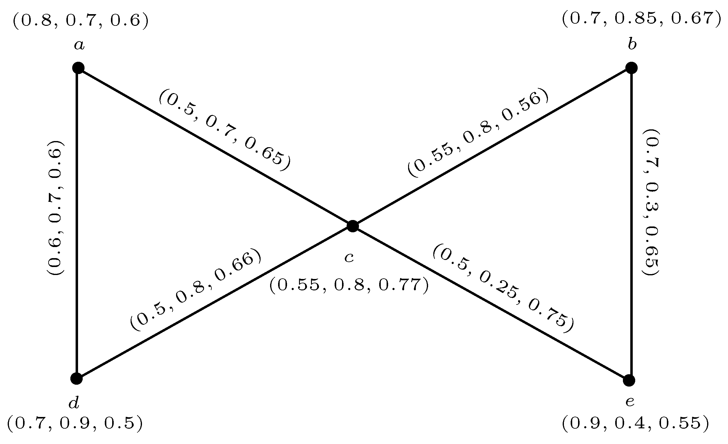
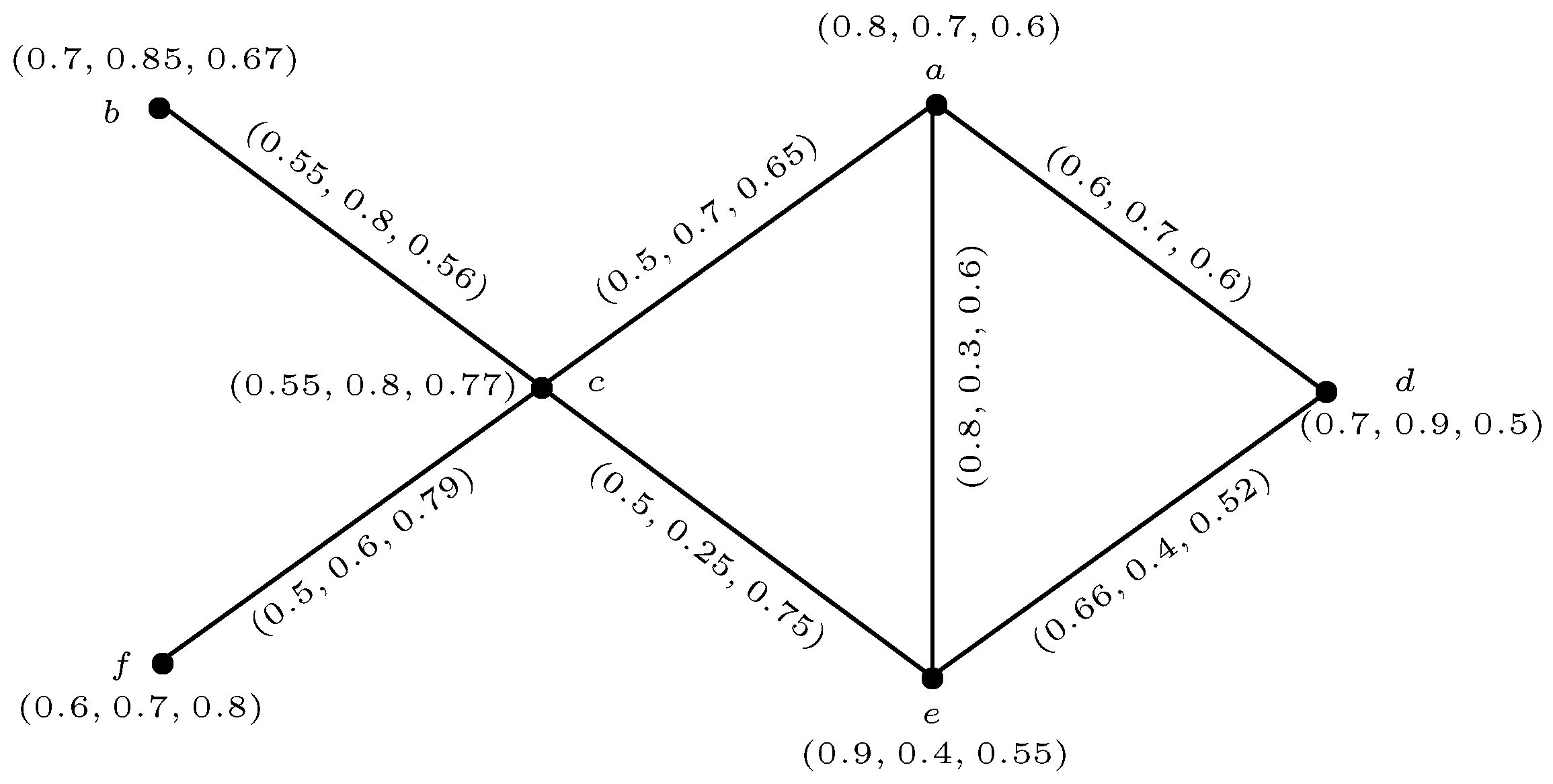
Definition 2. 

A q-rung picture fuzzy graph on a non-empty set X is a pair $\mathcal{G}=(\mathcal{P},\mathcal{Q})$ with $\mathcal{P}$ a q-rung picture fuzzy set on $X,$ and $\mathcal{Q}$ a q-rung picture fuzzy relation on X such that

$$\left\{\begin{array}{c}{\mu }_{\mathcal{Q}}(uv)\le {\mu }_{\mathcal{P}}(u)\wedge {\mu }_{\mathcal{P}}(v),\hfill \\ {\eta }_{\mathcal{Q}}(uv)\le {\eta }_{\mathcal{P}}(u)\wedge {\eta }_{\mathcal{P}}(v),\hfill \\ {\nu }_{\mathcal{Q}}(uv)\le {\nu }_{\mathcal{P}}(u)\vee {\nu }_{\mathcal{P}}(v),\hfill \end{array}\right.$$

and $0\le {\mu }_{\mathcal{Q}}^q(uv)+{\eta }_{\mathcal{Q}}^q(uv)+{\nu }_{\mathcal{Q}}^q(uv)\le 1$ for all $u,v\in X$, where ${\mu }_{\mathcal{Q}}:X\times X⟶[0,1],{\eta }_{\mathcal{Q}}:X\times X⟶[0,1]$ and ${\nu }_{\mathcal{Q}}:X\times X⟶[0,1]$ represents the positive membership, neutral membership, and negative membership functions of $\mathcal{Q}$, respectively.

Example 1. 

Consider a graph $G=(P,Q)$ such that $P=\{a,b,c,d,e\}$ and $Q=\{ac,ad,bc,be,cd,ce\}\subseteq P\times P.$ Let $\mathcal{P}$ be a 4-RPFS on P and $\mathcal{Q}$ be a 4-RPFR on $P,$ defined by

$\mathcal{P}$	a	b	c	d	e		$\mathcal{Q}$	$ac$	$ad$	$bc$	$be$	$cd$	$ce$
${\mu }_{\mathcal{P}}$	0.8	0.7	0.55	0.7	0.9		${\mu }_{\mathcal{Q}}$	0.5	0.6	0.55	0.7	0.5	0.5
${\eta }_{\mathcal{P}}$	0.7	0.85	0.8	0.9	0.4		${\eta }_{\mathcal{Q}}$	0.7	0.7	0.8	0.3	0.8	0.25
${\nu }_{\mathcal{P}}$	0.6	0.67	0.77	0.5	0.55		${\nu }_{\mathcal{Q}}$	0.65	0.6	0.56	0.65	0.66	0.75

Routine computations show that $\mathcal{G}=(\mathcal{P},\mathcal{Q}),$ displayed in Figure 2, is a 4-RPFG.

Definition 3. 

Let $\mathcal{G}=(\mathcal{P},\mathcal{Q})$ be a q-RPFG on underlying crisp graph $G=(P,Q)$. If ${\mu }_{\mathcal{Q}}(uv)={\mu }_{\mathcal{P}}(u)\wedge {\mu }_{\mathcal{P}}(v),{\eta }_{\mathcal{Q}}(uv)={\eta }_{\mathcal{P}}(u)\wedge {\eta }_{\mathcal{P}}(v)$ and ${\nu }_{\mathcal{Q}}(uv)={\nu }_{\mathcal{P}}(u)\vee {\nu }_{\mathcal{P}}(v)$ for all $uv\in Q$, then $\mathcal{G}=(\mathcal{P},\mathcal{Q})$ is called a strong q-rung picture fuzzy graph.

Definition 4. 

Let $\mathcal{G}=(\mathcal{P},\mathcal{Q})$ be a q-RPFG on underlying crisp graph $G=(P,Q)$. If ${\mu }_{\mathcal{Q}}(uv)={\mu }_{\mathcal{P}}(u)\wedge {\mu }_{\mathcal{P}}(v),{\eta }_{\mathcal{Q}}(uv)={\eta }_{\mathcal{P}}(u)\wedge {\eta }_{\mathcal{P}}(v)$ and ${\nu }_{\mathcal{Q}}(uv)={\nu }_{\mathcal{P}}(u)\vee {\nu }_{\mathcal{P}}(v)$ for all $u,v\in P$, then $\mathcal{G}=(\mathcal{P},\mathcal{Q})$ is called a complete q-rung picture fuzzy graph.

Definition 5. 

Let $\mathcal{G}=(\mathcal{P},\mathcal{Q})$ be a q-RPFG defined on $G=(P,Q).$ The order of $\mathcal{G}$ is denoted by $O(\mathcal{G}),$ and defined as

$$O(\mathcal{G})=\left(\sum _{u\in P}{\mu }_{\mathcal{P}}(u),\sum _{u\in P}{\eta }_{\mathcal{P}}(u),\sum _{u\in P}{\nu }_{\mathcal{P}}(u)\right).$$

Definition 6. 

Let $\mathcal{G}=(\mathcal{P},\mathcal{Q})$ be a q-RPFG defined on $G=(P,Q).$ The size of $\mathcal{G}$ is denoted by $S(\mathcal{G}),$ and defined as

$$S(\mathcal{G})=\left(\sum _{uv\in P}{\mu }_{\mathcal{Q}}(uv),\sum _{uv\in P}{\eta }_{\mathcal{Q}}(uv),\sum _{uv\in P}{\nu }_{\mathcal{Q}}(uv)\right).$$

Example 2. 

The order and size of q-rung picture fuzzy graph displayed in Figure 2 are $O(\mathcal{G})=(3.65,3.65,3.09)$ and $S(\mathcal{G})=(3.35,3.55,3.12),$ respectively.

Definition 7. 

Let $\mathcal{G}=(\mathcal{P},\mathcal{Q})$ be a q-RPFG defined on $G=(P,Q).$ The degree of a vertex u of $\mathcal{G}$ is denoted by $d_{\mathcal{G}}(u)=(d_{\mu }(u),d_{\eta }(u),d_{\nu }(u)),$ and defined as

$$d_{\mathcal{G}}(u)=\left(\sum _{uv\in Q}{\mu }_{\mathcal{Q}}(uv),\sum _{uv\in Q}{\eta }_{\mathcal{Q}}(uv),\sum _{uv\in Q}{\nu }_{\mathcal{Q}}(uv)\right).$$

Definition 8. 

Let $\mathcal{G}=(\mathcal{P},\mathcal{Q})$ be a q-RPFG defined on $G=(P,Q).$ The total degree of a vertex u of $\mathcal{G}$ is denoted by $t{d}_{\mathcal{G}}(u)=(t{d}_{\mu }(u),t{d}_{\eta }(u),t{d}_{\nu }(u)),$ and defined as

$$t{d}_{\mathcal{G}}(u)=\left(\sum _{uv\in Q}{\mu }_{\mathcal{Q}}(uv)+{\mu }_{\mathcal{P}}(u),\sum _{uv\in Q}{\eta }_{\mathcal{Q}}(uv)+{\eta }_{\mathcal{P}}(u),\sum _{uv\in Q}{\nu }_{\mathcal{Q}}(uv)+{\nu }_{\mathcal{P}}(u)\right).$$

Example 3. 

Consider a 4-RPFG $\mathcal{G}$ displayed in Figure 2. The degree, and total degree of vertex a in $\mathcal{G}$ is given as $d_{\mathcal{G}}(a)=({\mu }_{\mathcal{Q}}(ac)+{\mu }_{\mathcal{Q}}(ad),{\eta }_{\mathcal{Q}}(ac)+{\eta }_{\mathcal{Q}}(ad),{\nu }_{\mathcal{Q}}(ac)+{\nu }_{\mathcal{Q}}(ad))=(0.5+0.6,0.7+0.7,0.65+0.6)=(1.1,1.4,1.25),$ and $t{d}_{\mathcal{G}}(a)=(d_{\mu }(a)+{\mu }_{\mathcal{P}}(a),d_{\eta }(a)+{\eta }_{\mathcal{P}}(a),d_{\nu }(a)+{\nu }_{\mathcal{P}}(a))=(1.1+0.8,1.4+0.7,1.25+0.6)=(1.9,2.1,1.85),$ respectively.

Definition 9. 

Let $\mathcal{G}=(\mathcal{P},\mathcal{Q})$ be a q-RPFG defined on $G=(P,Q).$ If each vertex of $\mathcal{G}$ has same degree, that is, $d_{\mathcal{G}}(u)=(k_1,k_2,k_3)$ for all $u\in P,$ then $\mathcal{G}$ is called $(k_1,k_2,k_3)$-regular q-RPFG.

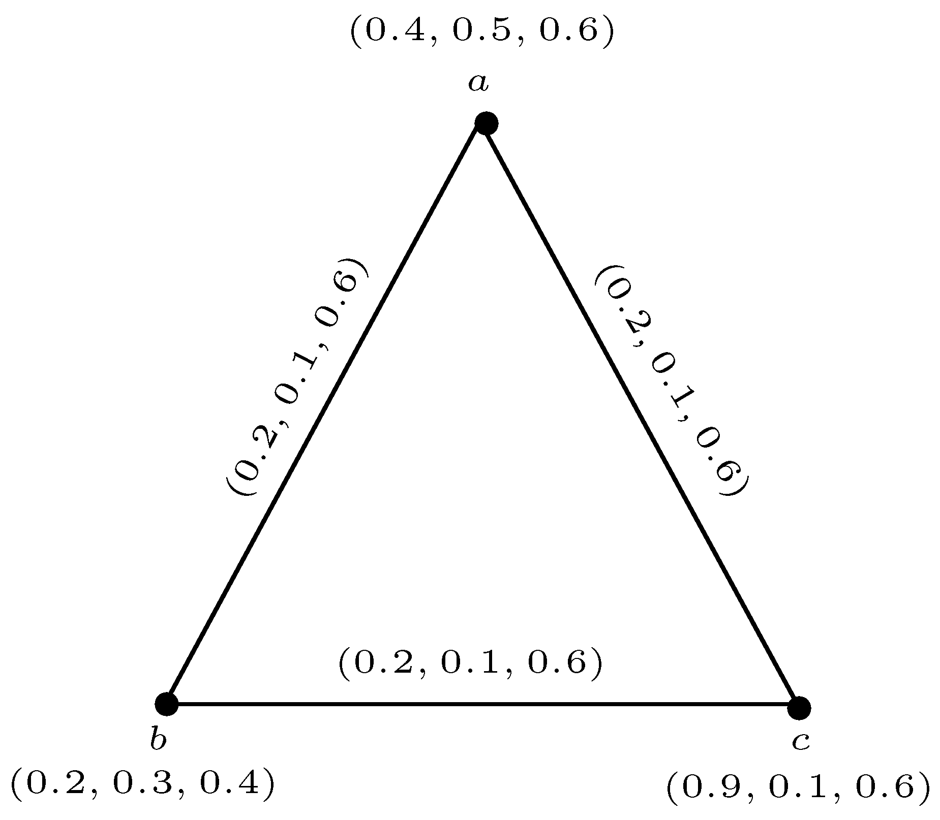
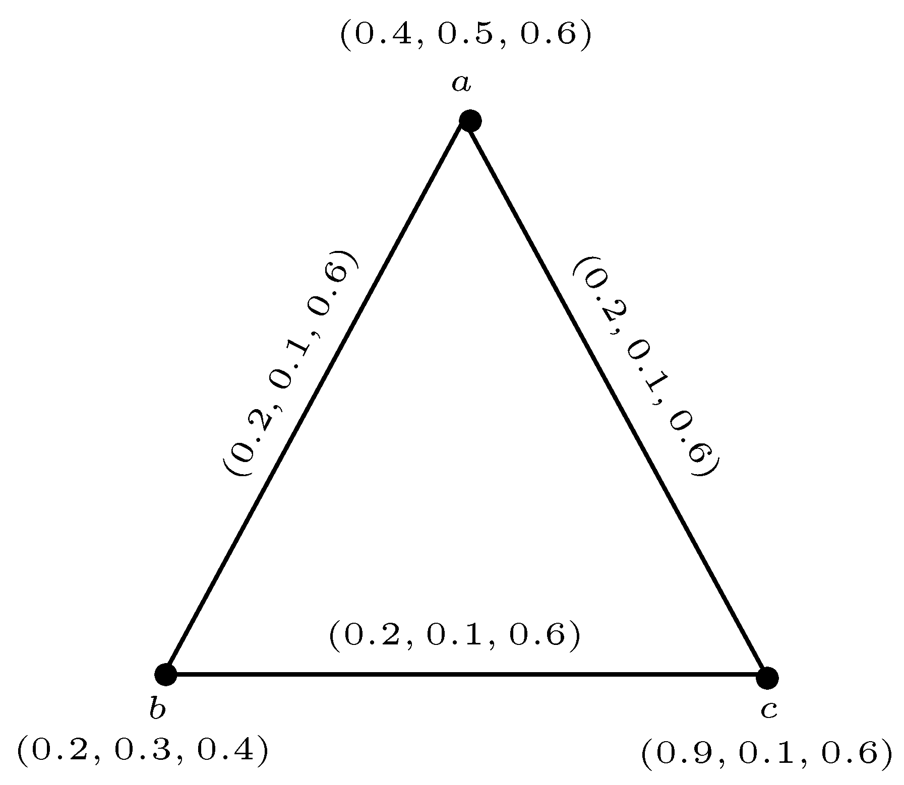
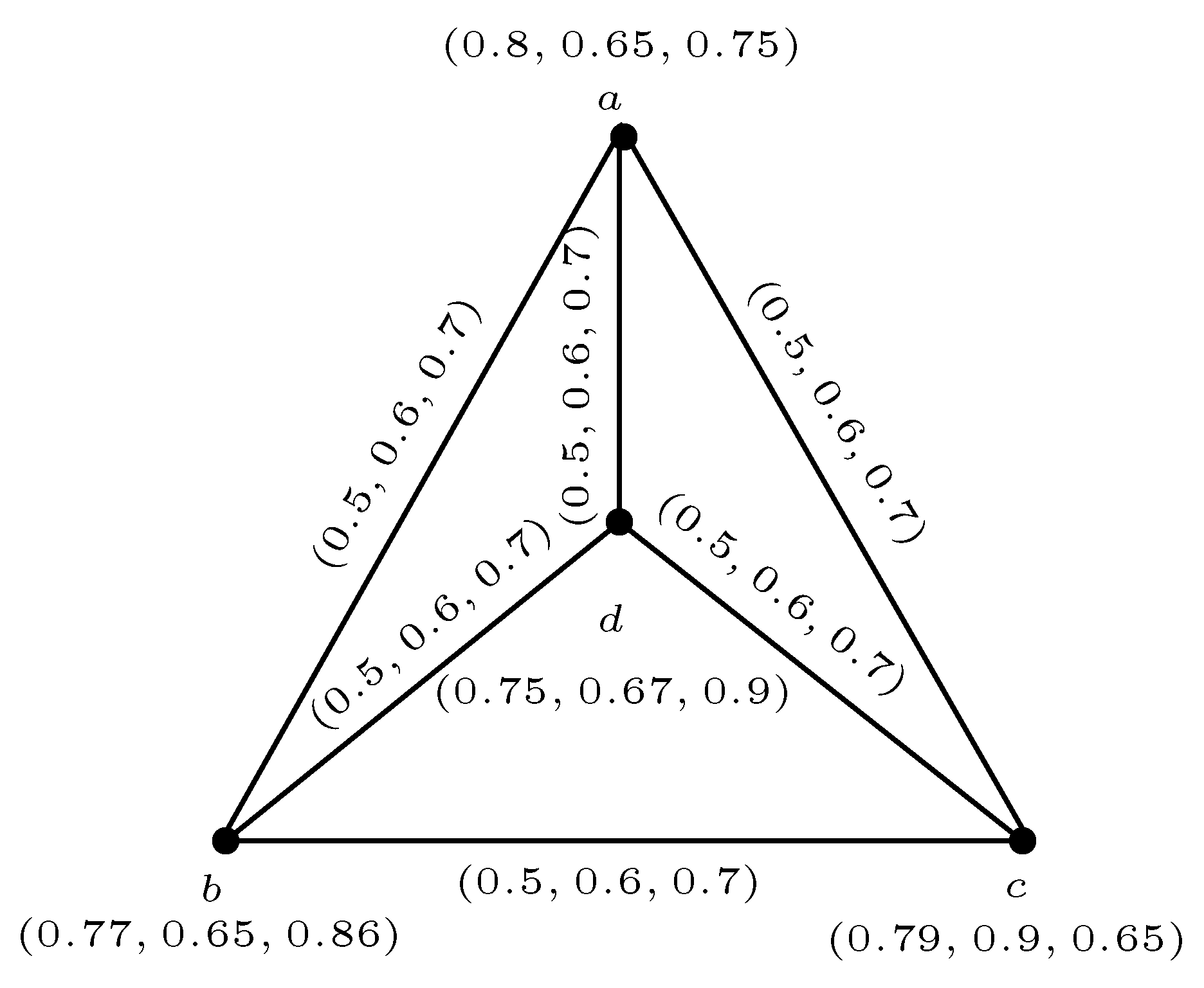
Example 4. 

Consider a 3-RPFG $\mathcal{G}=(\mathcal{P},\mathcal{Q})$ as displayed in Figure 3.

We see that the degree of each vertex in $\mathcal{G}$ is $d_{\mathcal{G}}(a)=d_{\mathcal{G}}(b)=d_{\mathcal{G}}(c)=(0.4,0.2,1.2).$ Hence, $\mathcal{G}$ is $(0.2,0.1,0.6)$-regular.

Definition 10. 

Let $\mathcal{G}=(\mathcal{P},\mathcal{Q})$ be a q-RPFG defined on $G=(P,Q).$ If each vertex of $\mathcal{G}$ has same total degree, that is, $t{d}_{\mathcal{G}}(u)=(l_1,l_2,l_3)$ for all $u\in P,$ then $\mathcal{G}$ is called $(l_1,l_2,l_3)$-totally regular q-RPFG.

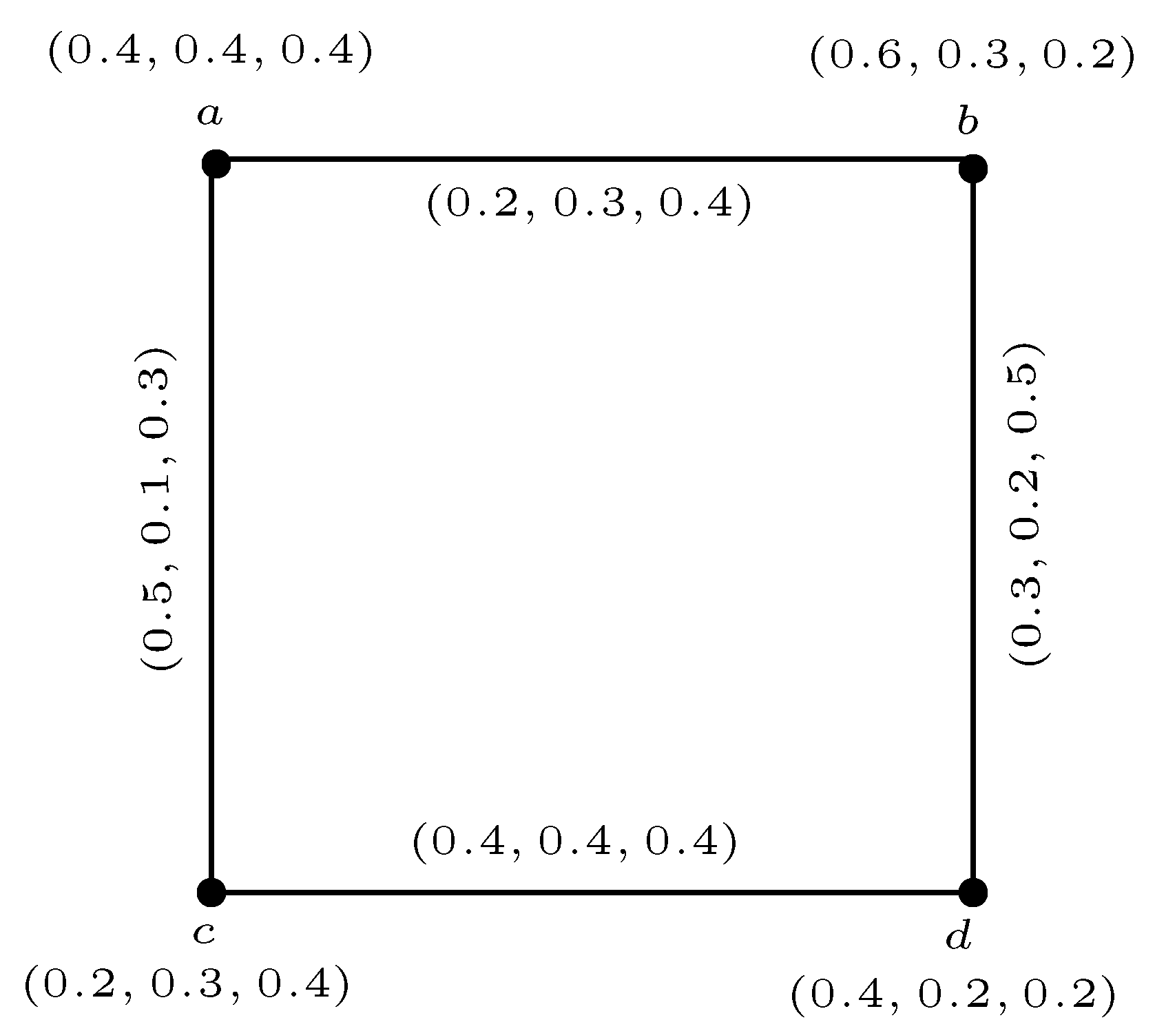
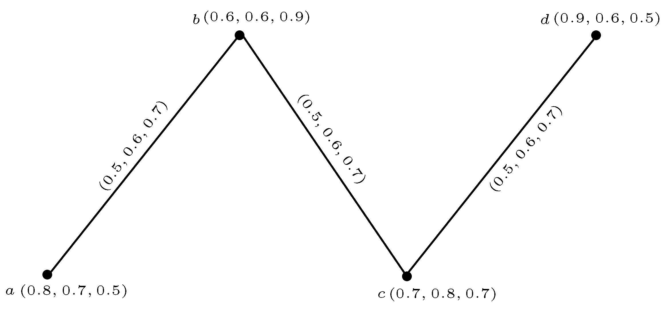
Example 5. 

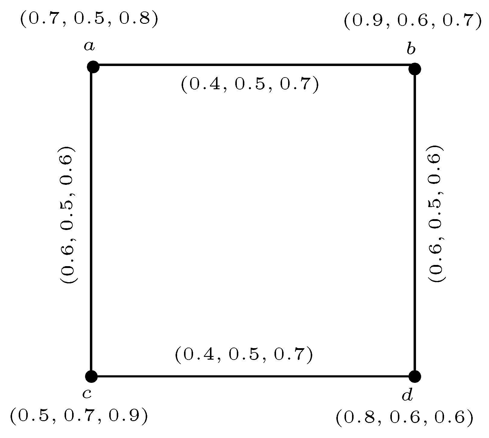
Consider a 2-RPFG $\mathcal{G}=(\mathcal{P},\mathcal{Q})$ as displayed in Figure 4.

$\mathcal{G}$ is $(1.1,0.8,1.1)$-totally regular 2-RPFG since $t{d}_{\mathcal{G}}(a)=t{d}_{\mathcal{G}}(b)=t{d}_{\mathcal{G}}(c)=t{d}_{\mathcal{G}}(d)=(1.1,0.8.1.1).$

Definition 11. 

A perfectly regular q-RPFG is a q-RPFG that is both regular and totally regular.

Example 6. 

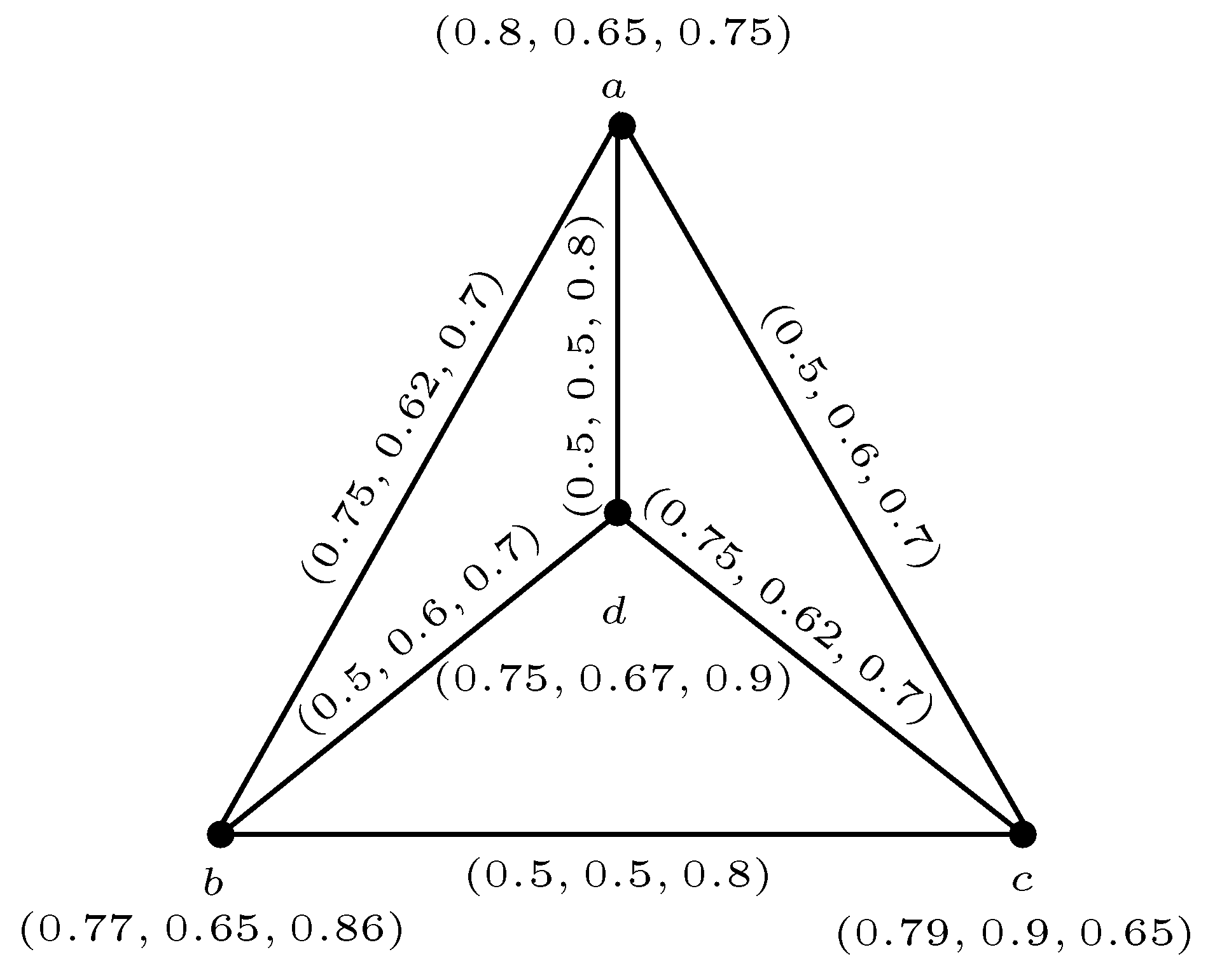
Consider a 3-rung picture fuzzy graph $\mathcal{G}=(\mathcal{P},\mathcal{Q})$ as shown in Figure 5.

Clearly, 3-RPFG $\mathcal{G}$ is regular since $d_{\mathcal{G}}(a)=d_{\mathcal{G}}(b)=d_{\mathcal{G}}(c)=d_{\mathcal{G}}(d)=(0.9,1.6,2.0),$ and is totally regular since $t{d}_{\mathcal{G}}(a)=t{d}_{\mathcal{G}}(b)=t{d}_{\mathcal{G}}(c)=t{d}_{\mathcal{G}}(d)=(1.4,2.2,2.8).$ Hence, $\mathcal{G}$ is perfectly regular 3-RPFG.

Definition 12. 

A q-RPFG $\mathcal{G}=(\mathcal{P},\mathcal{Q})$ defined on $G=(P,Q)$ is said to be partially regular if the underlying graph $G=(P,Q)$ is regular.

Definition 13. 

A q-RPFG $\mathcal{G}=(\mathcal{P},\mathcal{Q})$ defined on $G=(P,Q),$ is said to be full regular if $\mathcal{G}$ is both regular, and partially regular.

The concept of edge regularity has been explored by many researchers on fuzzy graphs, and several of its generalizations. We now give a description on edge regular q-RPFGs. First, we state some definitions in this context.

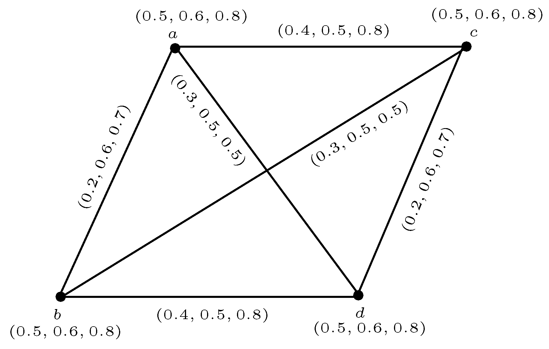
Definition 14. 

Let $\mathcal{G}=(\mathcal{P},\mathcal{Q})$ be a q-RPFG defined on $G=(P,Q).$ The edge degree of $uv$ in $\mathcal{G}$ is denoted by $d_{\mathcal{G}}(uv)=(d_{\mu }(uv),d_{\eta }(uv),d_{\nu }(uv)),$ and defined as

$$d_{\mathcal{G}}(uv)=d_{\mathcal{G}}(u)+d_{\mathcal{G}}(v)-2({\mu }_{\mathcal{Q}}(uv),{\eta }_{\mathcal{Q}}(uv),{\nu }_{\mathcal{Q}}(uv)).$$

This is equivalent to

$$\begin{array}{c}\hfill \begin{array}{cc}\hfill d_{\mathcal{G}}(uv)& =\left(\sum _{uw\in Q}{\mu }_{\mathcal{Q}}(uw),\sum _{uw\in Q}{\eta }_{\mathcal{Q}}(uw),\sum _{uw\in Q}{\nu }_{\mathcal{Q}}(uw)\right)+\left(\sum _{vw\in Q}{\mu }_{\mathcal{Q}}(vw),\sum _{vw\in Q}{\eta }_{\mathcal{Q}}(vw),\sum _{vw\in Q}{\nu }_{\mathcal{Q}}(vw)\right)\hfill \\ & -2({\mu }_{\mathcal{Q}}(uv),{\eta }_{\mathcal{Q}}(uv),{\nu }_{\mathcal{Q}}(uv))\hfill \\ & =\left(\sum _{w\ne v}{\mu }_{\mathcal{Q}}(uw),\sum _{w\ne v}{\eta }_{\mathcal{Q}}(uw),\sum _{w\ne v}{\nu }_{\mathcal{Q}}(uw)\right)+\left(\sum _{w\ne u}{\mu }_{\mathcal{Q}}(vw),\sum _{w\ne u}{\eta }_{\mathcal{Q}}(vw),\sum _{w\ne u}{\nu }_{\mathcal{Q}}(vw)\right).\hfill \end{array}\end{array}$$

Example 7. 

Consider a 4-RPFG $\mathcal{G}$ displayed in Figure 6.

The degree of edge $ad$ in $\mathcal{G}$ can be computed as

$$\begin{array}{ccc}\hfill d_{\mathcal{G}}(ad)& =& d_{\mathcal{G}}(a)+d_{\mathcal{G}}(d)-2({\mu }_{\mathcal{Q}}(ad),{\eta }_{\mathcal{Q}}(ad),{\nu }_{\mathcal{Q}}(ad))\hfill \\ & =& (1.9,1.7,1.85)+(1.26,1.1,1.12)-2(0.6,0.7,0.6)=(1.96,1.4,1.77).\hfill \end{array}$$

Theorem 1. 

[35] For any q-RPFG $\mathcal{G}=(\mathcal{P},\mathcal{Q})$ defined on $P=\{v_1,v_2,\dots ,v_n\},$ the following relation for degrees of vertices of $\mathcal{G}$ must hold:

$$\begin{array}{ccc}\hfill \sum _{j=1}^n{d}_{\mathcal{G}}(v_j)& =& 2\left(\sum _{\begin{array}{c}j=1\\ i>j\end{array}}^{n-1}{\mu }_{\mathcal{Q}}(v_j{v}_i),\sum _{\begin{array}{c}j=1\\ i>j\end{array}}^{n-1}{\eta }_{\mathcal{Q}}(v_j{v}_i),\sum _{\begin{array}{c}j=1\\ i>j\end{array}}^{n-1}{\nu }_{\mathcal{Q}}(v_j{v}_i)\right)\hfill \end{array}$$

for all $1\le i\le n.$

The following theorem is developed to define a comprehensive relationship between the degrees of edges, and the degrees of vertices of q-RPFGs.

Theorem 2. 

For any q-RPFG $\mathcal{G}=(\mathcal{P},\mathcal{Q})$ defined on $P=\{v_1,v_2,\dots ,v_n\},$ if$({\mu }_{\mathcal{Q}}(v_i{v}_j),{\eta }_{\mathcal{Q}}(v_i{v}_j),{\nu }_{\mathcal{Q}}(v_i{v}_j))\ne (0,0,0)$ for all $v_i,v_j\in P(i\ne j),$ then the following relation for degrees of edges of $\mathcal{G}$ must hold:

$$\begin{array}{ccc}\hfill \sum _{\begin{array}{c}i=1\\ j>i\end{array}}^{n-1}{d}_{\mathcal{G}}(v_i{v}_j)& =& (n-2)\sum _{i=1}^n{d}_{\mathcal{G}}(v_i)\hfill \end{array}$$

for all $1\le j\le n.$ That is, the sum of degrees of all edges is equal to $(n-2)$ times the sum of degrees of all vertices of $\mathcal{G}.$

Proof 

Let $P=\{v_1,v_2,\dots ,v_n\},$ and $\mathcal{G}=(\mathcal{P},\mathcal{Q})$ be a q-RPFG defined on $G=(P,Q).$ The degree of an edge $v_i{v}_j$ of q-RPFG $\mathcal{G}$ can be defined as

$$\begin{array}{ccc}\hfill d_{\mathcal{G}}(v_i{v}_j)& =& d_{\mathcal{G}}(v_i)+d_{\mathcal{G}}(v_j)-2({\mu }_{\mathcal{Q}}(v_i{v}_j),{\eta }_{\mathcal{Q}}(v_i{v}_j),{\nu }_{\mathcal{Q}}(v_i{v}_j)),\hfill \\ \hfill \sum _{\begin{array}{c}i,j=1\\ i\ne j\end{array}}^n{d}_{\mathcal{G}}(v_i{v}_j)& =& \sum _{\begin{array}{c}i,j=1\\ i\ne j\end{array}}^n{d}_{\mathcal{G}}(v_i)+\sum _{\begin{array}{c}i,j=1\\ i\ne j\end{array}}^n{d}_{\mathcal{G}}(v_j)-2\sum _{\begin{array}{c}i,j=1\\ i\ne j\end{array}}^n({\mu }_{\mathcal{Q}}(v_i{v}_j),{\eta }_{\mathcal{Q}}(v_i{v}_j),{\nu }_{\mathcal{Q}}(v_i{v}_j)).\hfill \end{array}$$

For all $1\le j\le n,$ we have

$$\begin{array}{ccc}\hfill 2\sum _{\begin{array}{c}i=1\\ j>i\end{array}}^{n-1}{d}_{\mathcal{G}}(v_i{v}_j)& =& (n-1)\sum _{i=1}^n{d}_{\mathcal{G}}(v_i)+(n-1)\sum _{j=1}^n{d}_{\mathcal{G}}(v_j)-2\left(2\sum _{\begin{array}{c}i=1\\ j>i\end{array}}^{n-1}({\mu }_{\mathcal{Q}}(v_i{v}_j),{\eta }_{\mathcal{Q}}(v_i{v}_j),{\nu }_{\mathcal{Q}}(v_i{v}_j))\right),\hfill \\ \hfill 2\sum _{\begin{array}{c}i=1\\ j>i\end{array}}^{n-1}{d}_{\mathcal{G}}(v_i{v}_j)& =& 2(n-1)\sum _{i=1}^n{d}_{\mathcal{G}}(v_i)-2\left[2\left(\sum _{\begin{array}{c}i=1\\ j>i\end{array}}^{n-1}{\mu }_{\mathcal{Q}}(v_i{v}_j),\sum _{\begin{array}{c}i=1\\ j>i\end{array}}^{n-1}{\eta }_{\mathcal{Q}}(v_i{v}_j),\sum _{\begin{array}{c}i=1\\ j>i\end{array}}^{n-1}{\nu }_{\mathcal{Q}}(v_i{v}_j)\right)\right],\hfill \\ \hfill 2\sum _{\begin{array}{c}i=1\\ j>i\end{array}}^{n-1}{d}_{\mathcal{G}}(v_i{v}_j)& =& 2(n-1)\sum _{i=1}^n{d}_{\mathcal{G}}(v_i)-2\sum _{i=1}^n{d}_{\mathcal{G}}(v_i),\mathrm{using}\mathrm{Theorem}1,\hfill \\ \hfill \sum _{\begin{array}{c}i=1\\ j>i\end{array}}^{n-1}{d}_{\mathcal{G}}(v_i{v}_j)& =& (n-2)\sum _{i=1}^n{d}_{\mathcal{G}}(v_i).\hfill \end{array}$$

This completes the proof. □

Next, we state some well known results regarding degrees of edges in q-RPFGs.

Theorem 3. 

Let $\mathcal{G}=(\mathcal{P},\mathcal{Q})$ be a q-RPFG on a cycle $G=(P,Q).$ Then,

$$\begin{array}{ccc}\hfill \sum _{v_i\in P}{d}_{\mathcal{G}}(v_i)& =& \sum _{v_i{v}_j\in Q}{d}_{\mathcal{G}}(v_i{v}_j).\hfill \end{array}$$

Theorem 4. 

Let $\mathcal{G}=(\mathcal{P},\mathcal{Q})$ be a q-RPFG on $G=(P,Q).$ Then,

$$\begin{array}{ccc}\hfill \sum _{v_i{v}_j\in Q}{d}_{\mathcal{G}}(v_i{v}_j)& =& \sum _{v_i{v}_j\in Q}{d}_G(v_i{v}_j)({\mu }_{\mathcal{Q}}(v_i{v}_j),{\eta }_{\mathcal{Q}}(v_i{v}_j),{\nu }_{\mathcal{Q}}(v_i{v}_j)),\hfill \end{array}$$

where $d_G(v_i{v}_j)=d_G(v_i)+d_G(v_j)-2$ for all $v_i,v_j\in P.$

Theorem 5. 

Let $\mathcal{G}=(\mathcal{P},\mathcal{Q})$ be a q-RPFG on a k-regular graph $G=(P,Q).$ Then,

$$\begin{array}{ccc}\hfill \sum _{v_i{v}_j\in Q}{d}_{\mathcal{G}}(v_i{v}_j)& =& 2(k-1)S(\mathcal{G}).\hfill \end{array}$$

For proofs of above theorems, readers are referred to [37,41,44].

Definition 15. 

The minimum edge degree of q-RPFG $\mathcal{G}$ is defined as ${\delta }_Q(\mathcal{G})=({{\delta }_Q}_{\mu }(\mathcal{G}),{{\delta }_Q}_{\eta }(\mathcal{G}),{{\delta }_Q}_{\nu }(\mathcal{G})),$ where ${{\delta }_Q}_{\mu }(\mathcal{G})=min\{d_{\mu }(uv):uv\in Q\}$ is minimum μ-edge degree of $\mathcal{G},{{\delta }_Q}_{\eta }(\mathcal{G})=min\{d_{\eta }(uv):uv\in Q\}$ is minimum η-edge degree of $\mathcal{G},$ and ${{\delta }_Q}_{\nu }(\mathcal{G})=min\{d_{\nu }(uv):uv\in Q\}$ is minimum ν-edge degree of $\mathcal{G}.$

Definition 16. 

The maximum edge degree of q-RPFG $\mathcal{G}$ is defined as ${\Delta }_Q(\mathcal{G})=({{\Delta }_Q}_{\mu }(\mathcal{G}),{{\Delta }_Q}_{\eta }(\mathcal{G}),{{\Delta }_Q}_{\nu }(\mathcal{G})),$ where ${{\Delta }_Q}_{\mu }(\mathcal{G})=max\{d_{\mu }(uv):uv\in Q\}$ is maximum μ-edge degree of $\mathcal{G},{{\Delta }_Q}_{\eta }(\mathcal{G})=max\{d_{\eta }(uv):uv\in Q\}$ is maximum η-edge degree of $\mathcal{G},$ and ${{\Delta }_Q}_{\nu }(\mathcal{G})=max\{d_{\nu }(uv):uv\in Q\}$ is maximum ν-edge degree of $\mathcal{G}.$

Example 8. 

Consider a q-rung picture fuzzy graph $\mathcal{G}=(\mathcal{P},\mathcal{Q})$ as shown in Figure 6. By routine computations, it is easy to see that the minimum, and maximum edge degree of $\mathcal{G}$ are ${\delta }_Q(\mathcal{G})=(1.55,1.25,1.87)and{\Delta }_Q(\mathcal{G})=(3.01,3.1,3.95).$

Definition 17. 

Let $\mathcal{G}=(\mathcal{P},\mathcal{Q})$ be a q-RPFG defined on $G=(P,Q).$ The total edge degree of $uv$ in $\mathcal{G}$ is denoted by $t{d}_{\mathcal{G}}(uv)=(t{d}_{\mu }(uv),t{d}_{\eta }(uv),t{d}_{\nu }(uv)),$ and defined as

$$t{d}_{\mathcal{G}}(uv)=d_{\mathcal{G}}(uv)+({\mu }_{\mathcal{Q}}(uv),{\eta }_{\mathcal{Q}}(uv),{\nu }_{\mathcal{Q}}(uv))=d_{\mathcal{G}}(u)+d_{\mathcal{G}}(v)-({\mu }_{\mathcal{Q}}(uv),{\eta }_{\mathcal{Q}}(uv),{\nu }_{\mathcal{Q}}(uv)).$$

This is equivalent to

$$\begin{array}{c}\hfill \begin{array}{cc}\hfill t{d}_{\mathcal{G}}(uv)& =\left(\sum _{w\ne v}{\mu }_{\mathcal{Q}}(uw),\sum _{w\ne v}{\eta }_{\mathcal{Q}}(uw),\sum _{w\ne v}{\nu }_{\mathcal{Q}}(uw)\right)+\left(\sum _{w\ne u}{\mu }_{\mathcal{Q}}(vw),\sum _{w\ne u}{\eta }_{\mathcal{Q}}(vw),\sum _{w\ne u}{\nu }_{\mathcal{Q}}(vw)\right)\hfill \\ & +({\mu }_{\mathcal{Q}}(uv),{\eta }_{\mathcal{Q}}(uv),{\nu }_{\mathcal{Q}}(uv)).\hfill \end{array}\end{array}$$

Example 9. 

Consider a 4-RPFG $\mathcal{G}$ displayed in Figure 6. The total degree of edge $ad$ in $\mathcal{G}$ can be computed as

$$\begin{array}{ccc}\hfill t{d}_{\mathcal{G}}(ad)& =& d_{\mathcal{G}}(ad)+({\mu }_{\mathcal{Q}}(ad),{\eta }_{\mathcal{Q}}(ad),{\nu }_{\mathcal{Q}}(ad))\hfill \\ & =& (1.96,1.4,1.77)+(0.6,0.7,0.6)=(2.56,2.1,2.37).\hfill \end{array}$$

Theorem 6. 

For any q-RPFG $\mathcal{G}=(\mathcal{P},\mathcal{Q})$ defined on $P=\{v_1,v_2,\dots ,v_n\},$ if $({\mu }_{\mathcal{Q}}(v_i{v}_j),$ ${\eta }_{\mathcal{Q}}(v_i{v}_j),$ ${\nu }_{\mathcal{Q}}(v_i{v}_j))\ne (0,0,0)$ for all $v_i,v_j\in P(i\ne j),$ then the following relation for total degrees of edges of $\mathcal{G}$ must hold:

$$\begin{array}{ccc}\hfill \sum _{\begin{array}{c}i=1\\ j>i\end{array}}^{n-1}t{d}_{\mathcal{G}}(v_i{v}_j)& =& \left(n-\frac{3}{2}\right)\sum _{i=1}^{n}t{d}_{\mathcal{G}}(v_i)\hfill \end{array}$$

for all $1\le j\le n.$

Proof. 

The proof directly follows from Theorem 2 and Definition 17. □

Theorem 7. 

Let $\mathcal{G}=(\mathcal{P},\mathcal{Q})$ be a q-RPFG on $G=(P,Q).$ Then,

$$\begin{array}{ccc}\hfill \sum _{v_i{v}_j\in Q}t{d}_{\mathcal{G}}(v_i{v}_j)& =& \sum _{v_i{v}_j\in Q}{d}_G(v_i{v}_j)({\mu }_{\mathcal{Q}}(v_i{v}_j),{\eta }_{\mathcal{Q}}(v_i{v}_j),{\nu }_{\mathcal{Q}}(v_i{v}_j))+S(\mathcal{G}),\hfill \end{array}$$

where $d_G(v_i{v}_j)=d_G(v_i)+d_G(v_j)-2$ for all $v_i,v_j\in P.$

Proof. 

The total degree of an edge $v_i{v}_j$ in a q-RPFG is

$$t{d}_{\mathcal{G}}(v_i{v}_j)=d_{\mathcal{G}}(v_i{v}_j)+({\mu }_{\mathcal{Q}}(v_i{v}_j),{\eta }_{\mathcal{Q}}(v_i{v}_j),{\nu }_{\mathcal{Q}}(v_i{v}_j)).$$

Therefore,

$$\begin{array}{ccc}\hfill \sum _{v_i{v}_j\in Q}t{d}_{\mathcal{G}}(v_i{v}_j)& =& \sum _{v_i{v}_j\in Q}(d_{\mathcal{G}}(v_i{v}_j)+({\mu }_{\mathcal{Q}}(v_i{v}_j),{\eta }_{\mathcal{Q}}(v_i{v}_j),{\nu }_{\mathcal{Q}}(v_i{v}_j)))\hfill \\ & =& \sum _{v_i{v}_j\in Q}{d}_{\mathcal{G}}(v_i{v}_j)+\sum _{v_i{v}_j\in Q}({\mu }_{\mathcal{Q}}(v_i{v}_j),{\eta }_{\mathcal{Q}}(v_i{v}_j),{\nu }_{\mathcal{Q}}(v_i{v}_j))\hfill \\ & =& \sum _{v_i{v}_j\in Q}{d}_G(v_i{v}_j)({\mu }_{\mathcal{Q}}(v_i{v}_j),{\eta }_{\mathcal{Q}}(v_i{v}_j),{\nu }_{\mathcal{Q}}(v_i{v}_j))+S(\mathcal{G}),\hfill \end{array}$$

where $d_G(v_i{v}_j)=d_G(v_i)+d_G(v_j)-2$ for all $v_i,v_j\in P.$ This completes the proof. □

The concept of edge degree leads to defining edge regularity of q-RPFGs. Formally, we have the following definition:

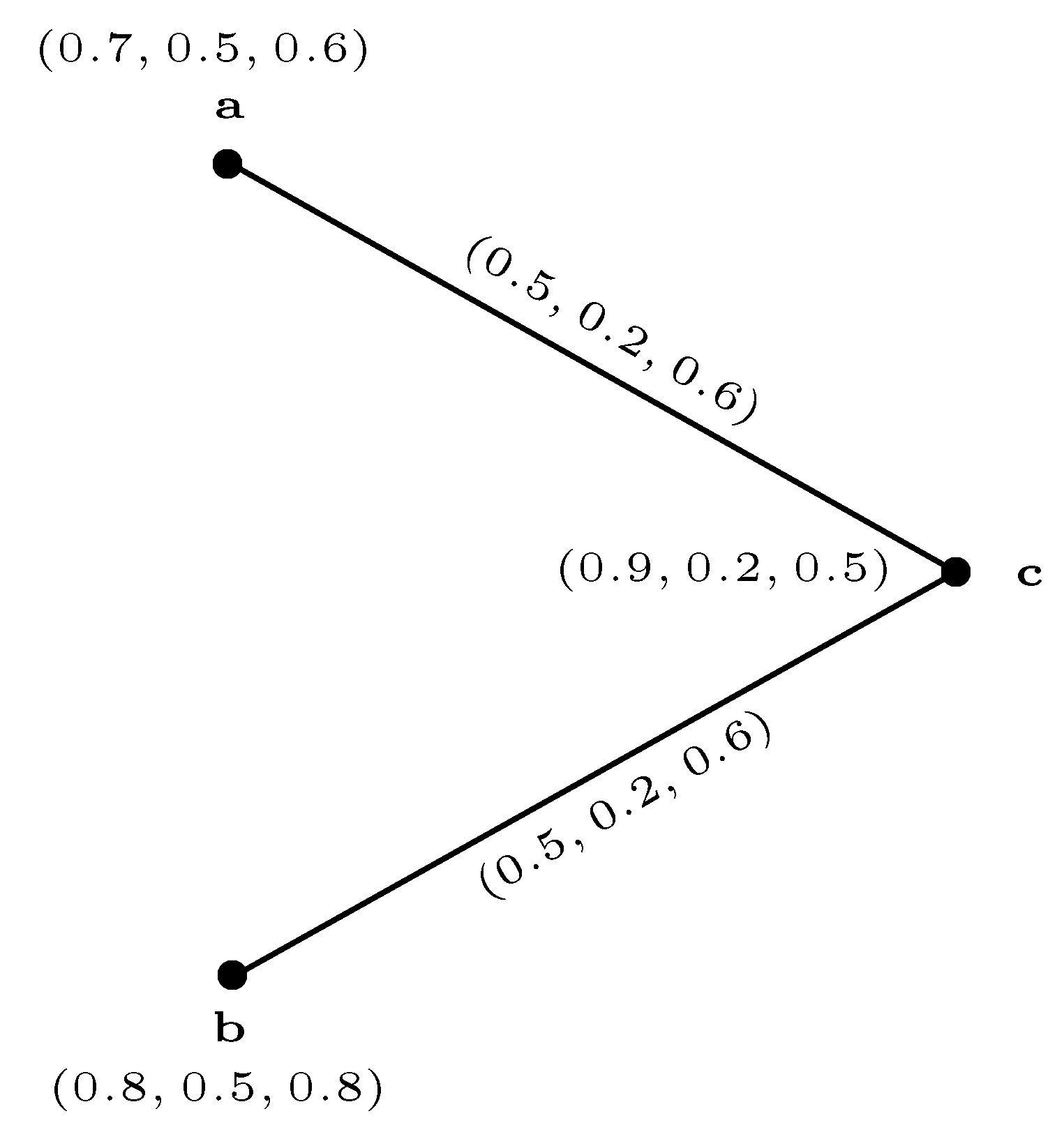
Definition 18. 

Let $\mathcal{G}=(\mathcal{P},\mathcal{Q})$ be a q-RPFG defined on $G=(P,Q).$ If each edge of $\mathcal{G}$ has same degree, which is

$$d_{\mathcal{G}}(uv)=(p_1,p_2,p_3)\mathrm{for}\mathrm{all}uv\in Q,$$

then $\mathcal{G}$ is called $(p_1,p_2,p_3)$-edge regular q-RPFG.

Example 10. 

Consider a 3-RPFG $\mathcal{G}=(\mathcal{P},\mathcal{Q})$ defined on $G=(P,Q),$ where $\mathcal{P}$ be a 3-rung picture fuzzy set on $P,$ and $\mathcal{Q}$ be a 3-rung picture fuzzy relation on $P,$ defined by

$\mathcal{P}$	a	b	c		$\mathcal{Q}$	$ab$	$bc$	$ac$
${\mu }_{\mathcal{P}}$	0.4	0.2	0.9		${\mu }_{\mathcal{Q}}$	0.2	0.2	0.2
${\eta }_{\mathcal{P}}$	0.5	0.3	0.1		${\eta }_{\mathcal{Q}}$	0.1	0.1	0.1
${\nu }_{\mathcal{P}}$	0.6	0.4	0.6		${\nu }_{\mathcal{Q}}$	0.6	0.6	0.6

We see that $d_{\mathcal{G}}(ab)=d_{\mathcal{G}}(bc)=d_{\mathcal{G}}(ac)=(0.4,0.2,1.2).$ Hence, the 3-RPFG $\mathcal{G},$ displayed in Figure 7, is $(0.4,0.2,1.2)$-edge regular.

Definition 19. 

Let $\mathcal{G}=(\mathcal{P},\mathcal{Q})$ be a q-RPFG defined on $G=(P,Q).$ If each edge of $\mathcal{G}$ has same total edge degree, that is

$$t{d}_{\mathcal{G}}(uv)=(q_1,q_2,q_3)\mathrm{for}\mathrm{all}uv\in Q,$$

then $\mathcal{G}$ is called $(q_1,q_2,q_3)$-total edge regular q-RPFG.

Example 11. 

Consider a 3-RPFG $\mathcal{G}=(\mathcal{P},\mathcal{Q})$ as displayed in Figure 8.

We see that $\mathcal{G}$ is $(1.3,1.2,0.9)$-total edge regular 3-RPFG since $t{d}_{\mathcal{G}}(ab)=t{d}_{\mathcal{G}}(bc)=t{d}_{\mathcal{G}}(ac)=(1.3,1.2.0.9).$

Remark 1. 

1. 

Any connected q-RPFG with two vertices is edge regular.

2. 

A q-RPFG is edge regular if and only if ${\delta }_Q(\mathcal{G})={\Delta }_Q(\mathcal{G}).$

Remark 2. 

A complete q-rung picture fuzzy graph need not be edge regular.

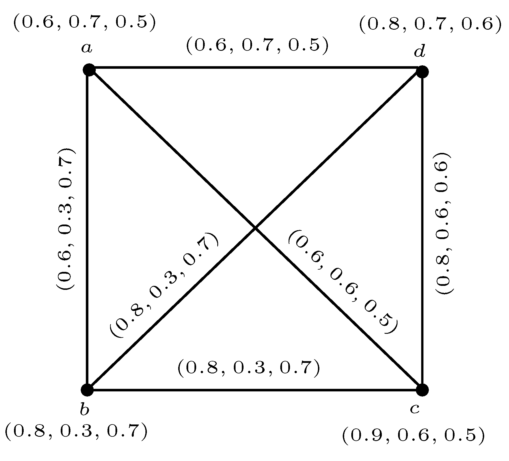
For example, consider a 4-RPFG $\mathcal{G}$ as displayed in Figure 9.

It is clear that $\mathcal{G}$ is a complete 4-RPFG. However, $\mathcal{G}$ is not edge regular since $d_{\mathcal{G}}(ab)=(2.8,1.9,2.4)\ne (2.8,1.8,2.5)=d_{\mathcal{G}}(ad).$

Next, we present a necessary condition for a complete q-RPFG to be edge regular.

Theorem 8. 

Let $\mathcal{G}=(\mathcal{P},\mathcal{Q})$ be a complete q-rung picture fuzzy graph on $G=(P,Q),$ and ${\mu }_{\mathcal{Q}},{\eta }_{\mathcal{Q}},$ and ${\nu }_{\mathcal{Q}}$ are constant functions; then, $\mathcal{G}$ is an edge regular q-RPFG.

Proof. 

Let $\mathcal{G}=(\mathcal{P},\mathcal{Q})$ be a complete q-rung picture fuzzy graph defined on $G=(P,Q),$ where $P=\{u_1,u_2,\dots ,u_n\}.$ Then, for all $u,v\in P,{\mu }_{\mathcal{Q}}(uv)={\mu }_{\mathcal{P}}(u)\wedge {\mu }_{\mathcal{P}}(v),{\eta }_{\mathcal{Q}}(uv)={\eta }_{\mathcal{P}}(u)\wedge {\eta }_{\mathcal{P}}(v),$ and ${\nu }_{\mathcal{Q}}(uv)={\nu }_{\mathcal{P}}(u)\vee {\nu }_{\mathcal{P}}(v).$ Let ${\mu }_{\mathcal{Q}}(uv)=c_1,{\eta }_{\mathcal{Q}}(uv)=c_{2}and{\nu }_{\mathcal{Q}}(uv)=c_3,$ for all $uv\in Q.$ The completeness of $\mathcal{G}$ implies that each vertex u of $\mathcal{G}$ is connected with $n-1$ vertices by edges, with membership values $({\mu }_{\mathcal{Q}}(uv),{\eta }_{\mathcal{Q}}(uv),{\nu }_{\mathcal{Q}}(uv))=(c_1,c_2,c_3).$ Thus, degree of each vertex $u\in P$ can be written as $d_{\mathcal{G}}(u)=(n-1)(c_1,c_2,c_3).$ By definition of edge degree, we have

$$\begin{array}{ccc}\hfill d_{\mathcal{G}}(uv)& =& d_{\mathcal{G}}(u)+d_{\mathcal{G}}(v)-2({\mu }_{\mathcal{Q}}(uv),{\eta }_{\mathcal{Q}}(uv),{\nu }_{\mathcal{Q}}(uv))\hfill \\ & =& (n-1)(c_1,c_2,c_3)+(n-1)(c_1,c_2,c_3)-2(c_1,c_2,c_3)\hfill \\ & =& 2(n-1)(c_1,c_2,c_3)-2(c_1,c_2,c_3)\hfill \\ & =& 2((n-2)c_1,(n-2)c_2,(n-2)c_3)\hfill \end{array}$$

for all $uv\in Q.$ Hence, $\mathcal{G}$ is an edge regular q-RPFG. This completes the proof. □

Remark 3. 

An edge regular q-rung picture fuzzy graph may not be total edge regular.

For example, consider a 6-RPFG $\mathcal{G}=(\mathcal{P},\mathcal{Q})$ as displayed in Figure 10.

We see that $\mathcal{G}$ is edge regular as $d_{\mathcal{G}}(ab)=d_{\mathcal{G}}(ac)=d_{\mathcal{G}}(bc)=d_{\mathcal{G}}(bd)=d_{\mathcal{G}}(cd)=(1.4,1.8,1.6).$ However, $\mathcal{G}$ is not total edge regular 6-RPFG since $t{d}_{\mathcal{G}}(ab)=(1.8,2.3,1.9)\ne (1.7,2.2,2.1)=t{d}_{\mathcal{G}}(cd).$

Remark 4. 

A total edge regular q-rung picture fuzzy graph may not be edge regular.

For example, consider a 3-rung picture fuzzy graph $\mathcal{G}=(\mathcal{P},\mathcal{Q})$ as displayed in Figure 8. We see that $\mathcal{G}$ is $(1.3,1.2,0.9)$-total edge regular. However, $\mathcal{G}$ is not an edge regular 3-RPFG since $d_{\mathcal{G}}(ab)=(0.9,0.8,0.4)\ne (0.9,0.8,0.7)=d_{\mathcal{G}}(ac).$

Moreover, it is easy to observe that there may exist such q-RPFGs which are both edge regular, and total edge regular—neither edge regular nor total edge regular. Thus, there does not exist any relationship between edge regular q-RPFGs, and total edge regular q-RPFGs. Next, we illustrate a theorem providing characterization for edge regularity of q-rung picture fuzzy graphs.

Theorem 9. 

Let $\mathcal{G}=(\mathcal{P},\mathcal{Q})$ be a q-rung picture fuzzy graph on $G=(P,Q),$ and ${\mu }_{\mathcal{Q}},{\eta }_{\mathcal{Q}},$ and ${\nu }_{\mathcal{Q}}$ are constant functions; then, the following are equivalent:

(a) 

$\mathcal{G}$ is an edge regular q-RPFG.

(b) 

$\mathcal{G}$ is a total edge regular q-RPFG.

Proof. 

Let $\mathcal{G}=(\mathcal{P},\mathcal{Q})$ be a q-RPFG on $G=(P,Q).$ Suppose that, for all $uv\in Q,{\mu }_{\mathcal{Q}}(uv)=c_1,{\eta }_{\mathcal{Q}}(uv)=c_2$ $\mathrm{and}{\nu }_{\mathcal{Q}}(uv)=c_3.$ Assume that $\mathcal{G}$ is a $(p_1,p_2,p_3)$-edge regular q-RPFG. Then, for all $uv\in Q,d_{\mathcal{G}}(uv)=(p_1,p_2,p_3).$ By definition of total edge degree,

$$\begin{array}{ccc}\hfill t{d}_{\mathcal{G}}(uv)& =& d_{\mathcal{G}}(uv)+({\mu }_{\mathcal{Q}}(uv),{\eta }_{\mathcal{Q}}(uv),{\nu }_{\mathcal{Q}}(uv))\hfill \\ & =& (p_1,p_2,p_3)+(c_1,c_2,c_3)\hfill \\ & =& (p_1+c_1,p_2+c_2,p_3+c_3)\hfill \end{array}$$

for all $uv\in Q.$ Hence, $\mathcal{G}$ is total edge regular q-RPFG.

Conversely, suppose that $\mathcal{G}$ is a $(q_1,q_2,q_3)$-total edge regular q-RPFG. Then, by definition of total edge regular

$$\begin{array}{ccc}\hfill t{d}_{\mathcal{G}}(uv)& =& d_{\mathcal{G}}(uv)+({\mu }_{\mathcal{Q}}(uv),{\eta }_{\mathcal{Q}}(uv),{\nu }_{\mathcal{Q}}(uv))\hfill \\ \hfill (q_1,q_2,q_3)& =& d_{\mathcal{G}}(uv)+(c_1,c_2,c_3)\hfill \\ \hfill d_{\mathcal{G}}(uv)& =& (q_1,q_2,q_3)-(c_1,c_2,c_3)\hfill \\ & =& (q_1-c_1,q_2-c_2,q_3-c_3)\hfill \end{array}$$

for all $uv\in Q.$ Hence, $\mathcal{G}$ is edge regular q-RPFG. This proves that $(a)$ and $(b)$ are equivalent.

On the other hand, assume that $(a),$ and $(b)$ are equivalent. Suppose, on the contrary, that ${\mu }_{\mathcal{Q}},{\eta }_{\mathcal{Q}},$ and ${\nu }_{\mathcal{Q}}$ are not constant functions. Then, there exist at least one edge $xy$ in Q such that $({\mu }_{\mathcal{Q}}(uv),{\eta }_{\mathcal{Q}}(uv),{\nu }_{\mathcal{Q}}(uv))\ne ({\mu }_{\mathcal{Q}}(xy),{\eta }_{\mathcal{Q}}(xy),and{\nu }_{\mathcal{Q}}(xy)).$ Let $\mathcal{G}$ be a $(p_1,p_2,p_3)$-edge regular q-RPFG. Then, $d_{\mathcal{G}}(uv)=d_{\mathcal{G}}(xy)=(p_1,p_2,p_3).$ Therefore,

$$\begin{array}{ccc}\hfill t{d}_{\mathcal{G}}(uv)& =& d_{\mathcal{G}}(uv)+({\mu }_{\mathcal{Q}}(uv),{\eta }_{\mathcal{Q}}(uv),{\nu }_{\mathcal{Q}}(uv))\hfill \\ & =& (p_1,p_2,p_3)+({\mu }_{\mathcal{Q}}(uv),{\eta }_{\mathcal{Q}}(uv),{\nu }_{\mathcal{Q}}(uv)),\hfill \end{array}$$

$$\begin{array}{ccc}\hfill t{d}_{\mathcal{G}}(xy)& =& d_{\mathcal{G}}(xy)+({\mu }_{\mathcal{Q}}(xy),{\eta }_{\mathcal{Q}}(xy),{\nu }_{\mathcal{Q}}(xy))\hfill \\ & =& (p_1,p_2,p_3)+({\mu }_{\mathcal{Q}}(xy),{\eta }_{\mathcal{Q}}(xy),{\nu }_{\mathcal{Q}}(xy)).\hfill \end{array}$$

Since $({\mu }_{\mathcal{Q}}(uv),{\eta }_{\mathcal{Q}}(uv),{\nu }_{\mathcal{Q}}(uv))\ne ({\mu }_{\mathcal{Q}}(xy),{\eta }_{\mathcal{Q}}(xy),{\nu }_{\mathcal{Q}}(xy)),$ therefore, $t{d}_{\mathcal{G}}(uv)\ne t{d}_{\mathcal{G}}(xy).$ Hence, $\mathcal{G}$ is not total edge regular, which gives a contradiction to our assumption.

Now, let $\mathcal{G}$ be a total edge regular q-RPFG. Then, by definition of total edge regular,

$$\begin{array}{ccc}\hfill t{d}_{\mathcal{G}}(uv)& =& t{d}_{\mathcal{G}}(xy),\hfill \\ \hfill d_{\mathcal{G}}(uv)+({\mu }_{\mathcal{Q}}(uv),{\eta }_{\mathcal{Q}}(uv),{\nu }_{\mathcal{Q}}(uv))& =& d_{\mathcal{G}}(xy)+({\mu }_{\mathcal{Q}}(xy),{\eta }_{\mathcal{Q}}(xy),{\nu }_{\mathcal{Q}}(xy)),\hfill \\ \hfill d_{\mathcal{G}}(uv)-d_{\mathcal{G}}(xy)& =& ({\mu }_{\mathcal{Q}}(xy),{\eta }_{\mathcal{Q}}(xy),{\nu }_{\mathcal{Q}}(xy))-({\mu }_{\mathcal{Q}}(uv),{\eta }_{\mathcal{Q}}(uv),{\nu }_{\mathcal{Q}}(uv))\ne 0,\hfill \\ \hfill d_{\mathcal{G}}(uv)& \ne & d_{\mathcal{G}}(xy).\hfill \end{array}$$

The fact that $\mathcal{G}$ is not edge regular leads a contradiction to our assumption. Hence, ${\mu }_{\mathcal{Q}},{\eta }_{\mathcal{Q}},$ and ${\nu }_{\mathcal{Q}}$ are constant functions. This completes the proof. □

Definition 20. 

A q-RPFG $\mathcal{G}=(\mathcal{P},\mathcal{Q})$ defined on $G=(P,Q)$ is said to be partially edge regular if the underlying graph $G=(P,Q)$ is edge regular.

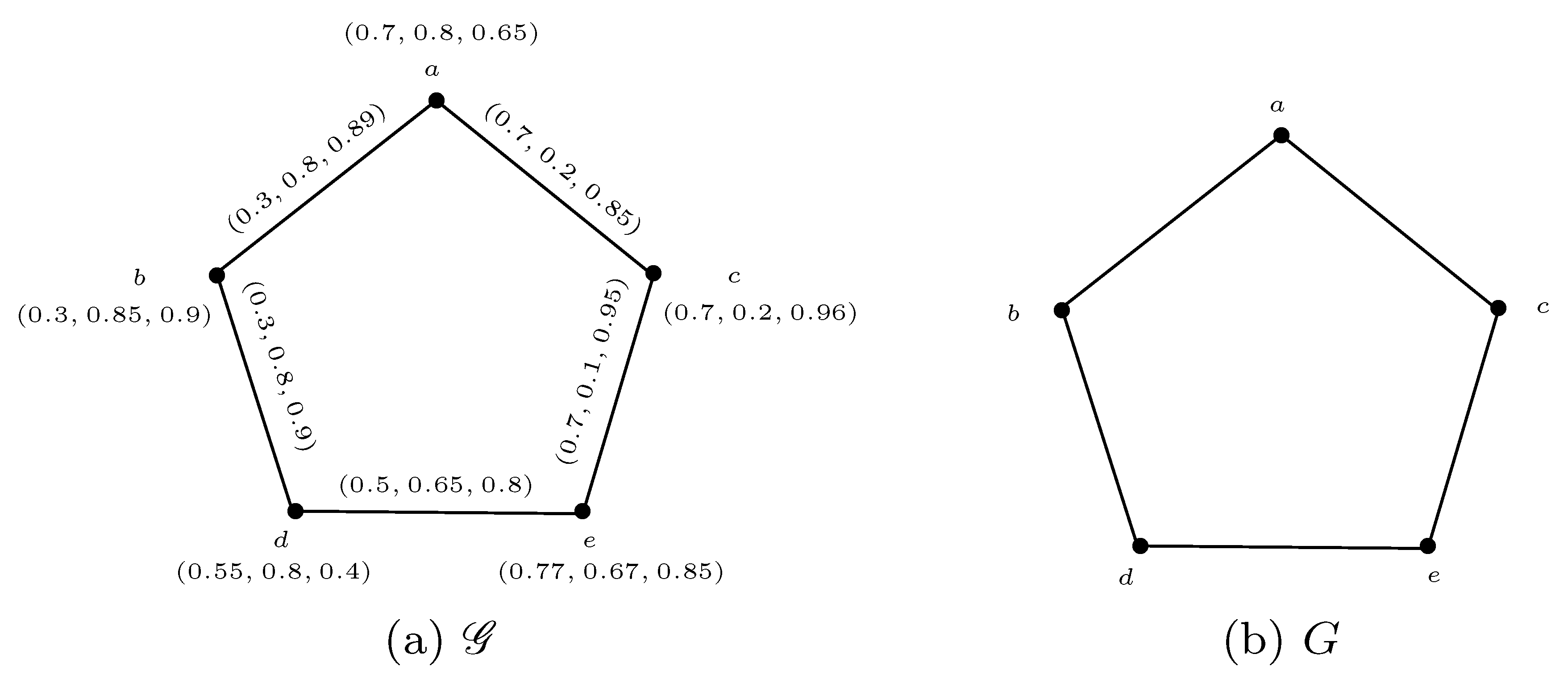
Example 12. 

Consider a 5-RPFG $\mathcal{G}=(\mathcal{P},\mathcal{Q})$ displayed in Figure 11a, and its underlying crisp graph $G=(P,Q)$ displayed in Figure 11b.

We see that G is 2-edge regular graph. Thus, $\mathcal{G}$ is partially edge regular 5-RPFG.

Definition 21. 

A q-RPFG $\mathcal{G}=(\mathcal{P},\mathcal{Q})$ defined on $G=(P,Q)$ is said to be full edge regular if $\mathcal{G}$ is both edge regular, and partially edge regular.

Example 13. 

Figure 7 can be considered as an example of full edge regular 3-RPFG. Since $\mathcal{G}$ as well as its underlying crisp graph G are edge regular.

Remark 5. 

An edge regular q-rung picture fuzzy graph may not be partially edge regular (or full edge regular).

For example, consider the 6-RPFG $\mathcal{G}=(\mathcal{P},\mathcal{Q}),$ displayed in Figure 12$a,$ and its underlying crisp graph $G=(P,Q)$ displayed in Figure 12$b.$

We see that $\mathcal{G}$ is edge regular as $d_{\mathcal{G}}(a)=d_{\mathcal{G}}(b)=d_{\mathcal{G}}(c)=d_{\mathcal{G}}(d)=d_{\mathcal{G}}(e)=(1.2,1.2,1.6).$ However, $\mathcal{G}$ is not partially edge regular 6-RPFG since its underlying graph $G=(P,Q)$ is not edge regular.

Remark 6. 

A partially edge regular q-rung picture fuzzy graph may not be edge regular (or full edge regular).

For example, consider a 5-RPFG $\mathcal{G}=(\mathcal{P},\mathcal{Q})$ displayed in Figure 11. We see that $\mathcal{G}$ is partially edge regular as its underlying graph G is edge regular. However, $\mathcal{G}$ is not edge regular 5-RPFG since $d_{\mathcal{G}}(ab)=(1.0,1.0,1.75)\ne (1.0,0.9,1.84)=d_{\mathcal{G}}(ac).$

The above remarks show that there does not exist any relationship between edge regular, and partially edge regular (or full edge regular) q-RPFGs. In the following theorem, we develop a relationship between edge regular, and partially edge regular q-RPFGs.

Theorem 10. 

Let $\mathcal{G}=(\mathcal{P},\mathcal{Q})$ be a q-rung picture fuzzy graph on $G=(P,Q).$ If ${\mu }_{\mathcal{Q}},{\eta }_{\mathcal{Q}},$ and ${\nu }_{\mathcal{Q}}$ are constant functions, then $\mathcal{G}$ is edge regular if and only if $\mathcal{G}$ is partially edge regular.

Proof. 

Let $\mathcal{G}=(\mathcal{P},\mathcal{Q})$ be a q-RPFG such that for all $uv\in Q,{\mu }_{\mathcal{Q}}(uv)=c_1,{\eta }_{\mathcal{Q}}(uv)=c_2\mathrm{and}{\nu }_{\mathcal{Q}}(uv)=c_3.$ Then, by definition of edge degree

$$\begin{array}{c}\hfill \begin{array}{cc}\hfill d_{\mathcal{G}}(uv)& =\left(\sum _{\begin{array}{c}uw\in Q\\ w\ne v\end{array}}{\mu }_{\mathcal{Q}}(uw),\sum _{\begin{array}{c}uw\in Q\\ w\ne v\end{array}}{\eta }_{\mathcal{Q}}(uw),\sum _{\begin{array}{c}uw\in Q\\ w\ne v\end{array}}{\nu }_{\mathcal{Q}}(uw)\right)+\left(\sum _{\begin{array}{c}vw\in Q\\ w\ne u\end{array}}{\mu }_{\mathcal{Q}}(vw),\sum _{\begin{array}{c}vw\in Q\\ w\ne u\end{array}}{\eta }_{\mathcal{Q}}(vw),\sum _{\begin{array}{c}vw\in Q\\ w\ne u\end{array}}{\nu }_{\mathcal{Q}}(vw)\right)\hfill \\ & =\sum _{\begin{array}{c}uw\in Q\\ w\ne v\end{array}}(c_1,c_2,c_3)+\sum _{\begin{array}{c}vw\in Q\\ w\ne u\end{array}}(c_1,c_2,c_3)\hfill \\ & =(c_1,c_2,c_3)(d_G(u)-1)+(c_1,c_2,c_3)(d_G(u)-1)\hfill \\ & =(c_1,c_2,c_3)(d_G(u)+d_G(v)-2)\hfill \\ & =(c_1,c_2,c_3)d_G(uv)\hfill \end{array}\end{array}$$

for all $uv\in Q.$ Hence, $\mathcal{G}$ is edge regular. Assume that $\mathcal{G}=(\mathcal{P},\mathcal{Q})$ is a $(p_1,p_2,p_3)$-edge regular q-RPFG. Then, for all $uv\in Q$,

$$\begin{array}{ccc}\hfill (p_1,p_2,p_3)& =& (c_1,c_2,c_3)d_G(uv),\hfill \\ \hfill d_G(uv)& =& \frac{(p_1,p_2,p_3)}{(c_1,c_2,c_3)}.\hfill \end{array}$$

This shows that G is an edge regular q-RPFG. Hence, $\mathcal{G}$ is partially edge regular q-RPFG.

Conversely, assume that $\mathcal{G}$ is partially edge regular q-RPFG. Let G be a p-edge regular graph. Then, for all $uv\in Q,$ $d_{\mathcal{G}}(uv)=p(c_1,c_2,c_3).$ Consequently, $\mathcal{G}$ is edge regular q-RPFG. This completes the proof. □

Corollary 1. 

Let $\mathcal{G}=(\mathcal{P},\mathcal{Q})$ be a q-RPFG such that ${\mu }_{\mathcal{Q}},{\eta }_{\mathcal{Q}},$ and ${\nu }_{\mathcal{Q}}$ are constant functions. If $\mathcal{G}$ is an edge regular q-RPFG or a partially edge regular q-RPFG, then $\mathcal{G}$ is a full edge regular q-RPFG.

Theorem 11. 

Let $\mathcal{G}=(\mathcal{P},\mathcal{Q})$ be a strong q-RPFG such that ${\mu }_{\mathcal{P}},{\eta }_{\mathcal{P}},$ and ${\nu }_{\mathcal{P}}$ are constant functions. Then, $\mathcal{G}$ is an edge regular q-RPFG if and only if $\mathcal{G}$ is partially edge regular q-RPFG.

Proof. 

Let $\mathcal{G}=(\mathcal{P},\mathcal{Q})$ be a strong q-RPFG defined on $G=(P,Q)$. Then, for all $uv\in Q,$ ${\mu }_{\mathcal{Q}}(uv)={\mu }_{\mathcal{P}}(u)\wedge {\mu }_{\mathcal{P}}(v),{\eta }_{\mathcal{Q}}(uv)={\eta }_{\mathcal{P}}(u)\wedge {\eta }_{\mathcal{P}}(v),$ and ${\nu }_{\mathcal{Q}}(uv)={\nu }_{\mathcal{P}}(u)\vee {\nu }_{\mathcal{P}}(v).$ Let ${\mu }_{\mathcal{P}},{\eta }_{\mathcal{P}},$ and ${\nu }_{\mathcal{P}}$ be constant functions. Then, for all $u\in P,{\mu }_{\mathcal{P}}(u)=c_1,{\eta }_{\mathcal{P}}(u)=c_2,$ and ${\nu }_{\mathcal{P}}(u)=c_3.$ Combining both facts, we have

$$\begin{array}{ccc}\hfill {\mu }_{\mathcal{Q}}(uv)& =& {\mu }_{\mathcal{P}}(u)\wedge {\mu }_{\mathcal{P}}(v)=c_1\wedge c_1=c_1,\hfill \\ \hfill {\eta }_{\mathcal{Q}}(uv)& =& {\eta }_{\mathcal{P}}(u)\wedge {\eta }_{\mathcal{P}}(v)=c_2\wedge c_2=c_2,\hfill \\ \hfill {\nu }_{\mathcal{Q}}(uv)& =& {\nu }_{\mathcal{P}}(u)\vee {\nu }_{\mathcal{P}}(v)=c_3\vee c_3=c_3.\hfill \end{array}$$

Thus, ${\mu }_{\mathcal{Q}},{\eta }_{\mathcal{Q}},$ and ${\nu }_{\mathcal{Q}}$ are constant functions. Consequently, the result follows from Theorem 10. □

Corollary 2. 

Let $\mathcal{G}=(\mathcal{P},\mathcal{Q})$ be a strong q-RPFG such that ${\mu }_{\mathcal{P}},{\eta }_{\mathcal{P}},$ and ${\nu }_{\mathcal{P}}$ are constant functions. If $\mathcal{G}$ is an edge regular q-RPFG or a partially edge regular q-RPFG, then $\mathcal{G}$ is a full edge regular q-RPFG.

Next, we state some results regarding order, and size of edge regular q-RPFG.

Theorem 12. 

The size of $(p_1,p_2,p_3)$-edge regular q-RPFG $\mathcal{G}=(\mathcal{P},\mathcal{Q})$ on a p-edge regular graph $G=(P,Q)$ is $\frac{q(p_1,p_2,p_3)}{p},$ where $q=\left|Q\right|.$

Theorem 13. 

If $\mathcal{G}=(\mathcal{P},\mathcal{Q})$ is $(q_1,q_2,q_3)$-total edge regular, and $(r_1,r_2,r_3)$-partially edge regular q-RPFG, then $S(\mathcal{G})=\frac{q(q_1,q_2,q_3)}{(r_1,r_2,r_3)+1},$ where $q=\left|Q\right|.$

Theorem 14. 

If $\mathcal{G}=(\mathcal{P},\mathcal{Q})$ is $(p_1,p_2,p_3)$-edge regular, and $(q_1,q_2,q_3)$-total edge regular q-RPFG, then $S(\mathcal{G})=q(q_1-p_1,q_2-p_2,q_3-p_3),$ where $q=\left|Q\right|.$

For proofs of above results, readers are referred to [37,41].

2.1. Perfectly Edge Regular q-RPFGs

In this section, we introduce perfect edge regular q-RPFGs taking as a point of departure the respective definition of perfect edge regular fuzzy graphs by Cary [38].

Definition 22. 

A perfect edge regular q-RPFG is a q-RPFG that is both edge regular, and total edge regular.

Example 14. 

Consider a 5-rung picture fuzzy graph $\mathcal{G}=(\mathcal{P},\mathcal{Q})$ as shown in Figure 13.

Clearly, $\mathcal{G}$ is $(2.0,2.4,2.8)$-edge regular, and $(2.5,3.0,3.5)$-total edge regular. Hence, $\mathcal{G}$ is perfect edge regular 5-RPFG.

Theorem 15. 

If $\mathcal{G}=(\mathcal{P},\mathcal{Q})$ is perfect edge regular q-RPFG, then ${\mu }_{\mathcal{Q}},{\eta }_{\mathcal{Q}},$ and ${\nu }_{\mathcal{Q}}$ are constant functions.

Proof. 

Let $\mathcal{G}=(\mathcal{P},\mathcal{Q})$ be a perfect edge regular q-RPFG defined on $G=(P,Q).$ Then, $\mathcal{G}$ must be edge regular and total edge regular, i.e., for all $uv\in Q,d_{\mathcal{G}}(uv)=(p_1,p_2,p_3),$ and $t{d}_{\mathcal{G}}(uv)=(q_1,q_2,q_3).$ By definition of total edge degree,

$$\begin{array}{ccc}\hfill d_{\mathcal{G}}(uv)+({\mu }_{\mathcal{Q}}(uv),{\eta }_{\mathcal{Q}}(uv),{\nu }_{\mathcal{Q}}(uv))& =& (q_1,q_2,q_3),\hfill \\ \hfill (p_1,p_2,p_3)+({\mu }_{\mathcal{Q}}(uv),{\eta }_{\mathcal{Q}}(uv),{\nu }_{\mathcal{Q}}(uv))& =& (q_1,q_2,q_3),\hfill \\ \hfill ({\mu }_{\mathcal{Q}}(uv),{\eta }_{\mathcal{Q}}(uv),{\nu }_{\mathcal{Q}}(uv))& =& (q_1-p_1,q_2-p_2,q_3-p_3).\hfill \end{array}$$

Since ${\mu }_{\mathcal{Q}}(uv)=q_1-p_1,{\eta }_{\mathcal{Q}}(uv)=q_2-p_2,$ and ${\nu }_{\mathcal{Q}}(uv)=q_3-p_3,$ for all $uv\in Q,$ therefore, ${\mu }_{\mathcal{Q}},{\eta }_{\mathcal{Q}},$ and ${\nu }_{\mathcal{Q}}$ are constant functions. This completes the proof. □

Perfectly edge regular q-RPFGs can be classified by the following theorem.

Theorem 16. 

A q-RPFG $\mathcal{G}=(\mathcal{P},\mathcal{Q})$ is perfect edge regular if and only if it satisfies the following conditions:

1. 

${\sum }_{uw\in Q}\left({\mu }_{\mathcal{Q}}(uw),{\eta }_{\mathcal{Q}}(uw),{\nu }_{\mathcal{Q}}(uw)\right)+{\sum }_{vw\in Q}\left({\mu }_{\mathcal{Q}}(vw),{\eta }_{\mathcal{Q}}(vw),{\nu }_{\mathcal{Q}}(vw)\right)-2({\mu }_{\mathcal{Q}}(uv),{\eta }_{\mathcal{Q}}(uv),{\nu }_{\mathcal{Q}}(uv))={\sum }_{xz\in Q}\left({\mu }_{\mathcal{Q}}(xz),{\eta }_{\mathcal{Q}}(xz),{\nu }_{\mathcal{Q}}(xz)\right)+{\sum }_{yz\in Q}\left({\mu }_{\mathcal{Q}}(yz),{\eta }_{\mathcal{Q}}(yz),{\nu }_{\mathcal{Q}}(yz)\right)-2({\mu }_{\mathcal{Q}}(xy),{\eta }_{\mathcal{Q}}(xy),{\nu }_{\mathcal{Q}}(xy)),$

2. 

$({\mu }_{\mathcal{Q}}(uv),{\eta }_{\mathcal{Q}}(uv),{\nu }_{\mathcal{Q}}(uv))=({\mu }_{\mathcal{Q}}(xy),{\eta }_{\mathcal{Q}}(xy),{\nu }_{\mathcal{Q}}(xy)),$

for all $uv,xy\in Q.$

Proof. 

Suppose that $\mathcal{G}=(\mathcal{P},\mathcal{Q})$ is perfect edge regular q-RPFG. Then, it must be regular as well as total edge regular. The fact that $\mathcal{G}$ is edge regular implies Condition 1 so that each edge has the same degree. Condition 2 is followed directly by Theorem 15.

Conversely, suppose that Condition 1 and 2 hold. It is straightforward to see that Condition 1 guarantees the edge regularity of $\mathcal{G}.$ Let for any two edges $uv$ and $xy,$ $d_{\mathcal{G}}(uv)=d_{\mathcal{G}}(xy).$ By definition of total edge degree,

$$\begin{array}{ccc}\hfill t{d}_{\mathcal{G}}(uv)& =& d_{\mathcal{G}}(uv)+({\mu }_{\mathcal{Q}}(uv),{\eta }_{\mathcal{Q}}(uv),{\nu }_{\mathcal{Q}}(uv))\hfill \\ & =& d_{\mathcal{G}}(xy)+({\mu }_{\mathcal{Q}}(xy),{\eta }_{\mathcal{Q}}(xy),{\nu }_{\mathcal{Q}}(xy))=t{d}_{\mathcal{G}}(xy).\hfill \end{array}$$

Thus, $\mathcal{G}$ is total edge regular, as $uv$ and $xy$ are arbitrary edges. Consequently, $\mathcal{G}$ is perfect edge regular. This completes the proof. □

Remark 7. 

The above theorem does not constitute a sufficient condition for a q-RPFG to be perfect edge regular.

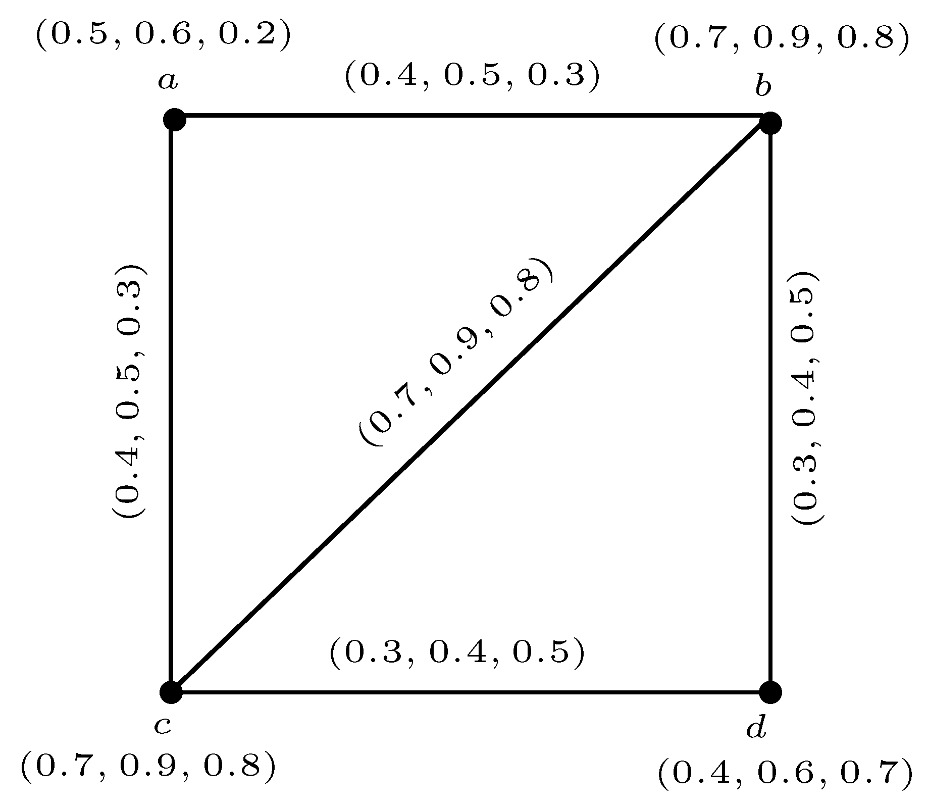
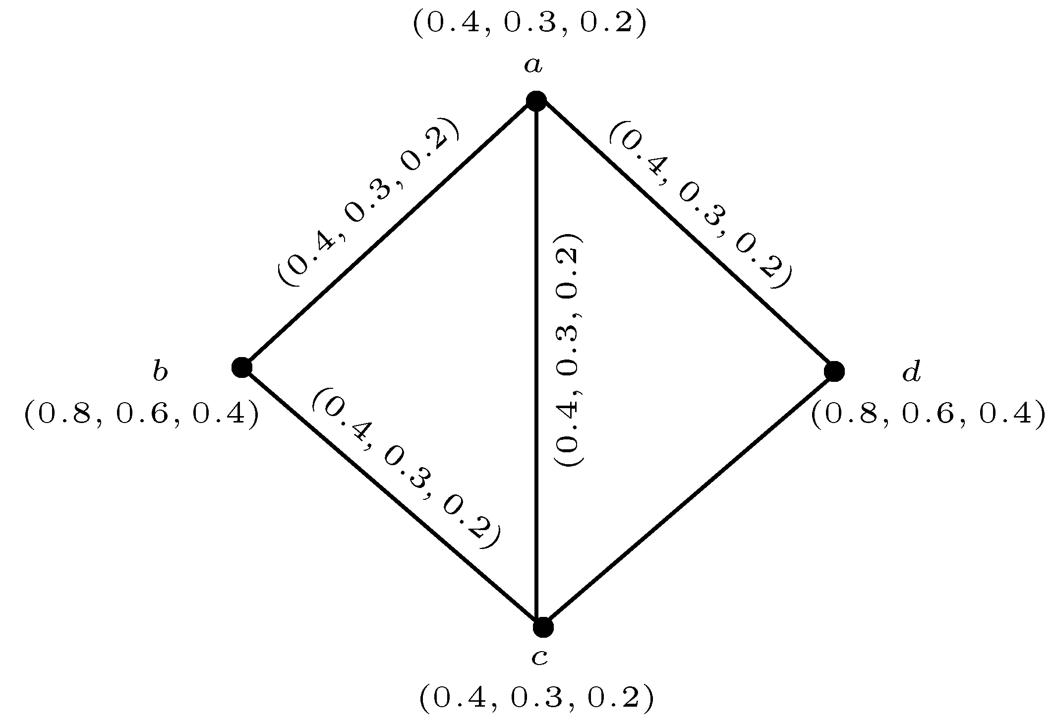
For example, consider a 4-RPFG $\mathcal{G}$ as displayed in Figure 14.

We see that $({\mu }_{\mathcal{Q}}(uv),{\eta }_{\mathcal{Q}}(uv),{\nu }_{\mathcal{Q}}(uv))=(0.5,0.6,0.7),$ for all $uv\in Q.$ However, since $d_{\mathcal{G}}(ab)=(0.5,0.6,0.7)\ne (1.0,1.2,1.4)=d_{\mathcal{G}}(bc),$ and $t{d}_{\mathcal{G}}(ab)=(1.0,1.2,1.4)\ne (1.5,1.8,2.1)=t{d}_{\mathcal{G}}(bc),$ therefore, $\mathcal{G}$ is neither edge regular nor totally egde regular. Hence, $\mathcal{G}$ is not a perfect edge regular 4-RPFG.

The following theorem provides a necessary condition for the converse of the above theorem to hold.

Theorem 17. 

If $\mathcal{G}=(\mathcal{P},\mathcal{Q})$ is edge regular q-RPFG, and ${\mu }_{\mathcal{Q}},{\eta }_{\mathcal{Q}},$ and ${\nu }_{\mathcal{Q}}$ are constant functions, then $\mathcal{G}$ is perfect edge regular q-RPFG.

Proof. 

The proof is directly followed from Theorem 9, which proves that $\mathcal{G}$ is total edge regular q-RPFG. Moreover, by our assumption, $\mathcal{G}$ is edge regular. Hence, $\mathcal{G}$ is perfect edge regular. This completes the proof. □

We next illustrate some results relating order and size of perfect edge regular q-RPFG.

Theorem 18. 

If $\mathcal{G}=(\mathcal{P},\mathcal{Q})$ is perfect edge regular q-RPFG, and ${\mu }_{\mathcal{Q}},{\eta }_{\mathcal{Q}},$ and ${\nu }_{\mathcal{Q}}$ are constant functions, then the size of $\mathcal{G}$ is $S(\mathcal{G})=(c_1,c_2,c_3)\left|Q\right|.$

Proof. 

Obvious. □

Unlike the order of perfectly regular q-RPFG, we can no longer give an explicit formula for the order of perfect edge regular q-RPFG. However, we can bound its order.

Theorem 19. 

If $\mathcal{G}=(\mathcal{P},\mathcal{Q})$ is perfect edge regular q-RPFG, then the order of $\mathcal{G}$ is bounded as:

$$\sum _{u\in P}\underset{u\ne v}{max}\{{\mu }_{\mathcal{Q}}(uv),{\eta }_{\mathcal{Q}}(uv),{\nu }_{\mathcal{Q}}(uv)\}\le O(\mathcal{G})\le \left|P\right|.$$

Proof. 

Upper bound of $O(\mathcal{G})$ is obvious. We now prove its lower bound. By definition of q-RPFG, ${\mu }_{\mathcal{Q}}(uv)\le {\mu }_{\mathcal{P}}(u)\wedge {\mu }_{\mathcal{P}}(v),{\eta }_{\mathcal{Q}}(uv)\le {\eta }_{\mathcal{P}}(u)\wedge {\eta }_{\mathcal{P}}(v),$ and ${\nu }_{\mathcal{Q}}(uv)\le {\nu }_{\mathcal{P}}(u)\vee {\nu }_{\mathcal{P}}(v).$ Thus, we have ${\mu }_{\mathcal{P}}(u)\ge {max}_{u\ne v}{\mu }_{\mathcal{Q}}(uv),$ ${\eta }_{\mathcal{P}}(u)\ge {max}_{u\ne v}{\eta }_{\mathcal{Q}}(uv),$ and ${\nu }_{\mathcal{P}}(u)\ge {max}_{u\ne v}{\nu }_{\mathcal{Q}}(uv).$ For each $u\in P,$ we obtain

$$\begin{array}{ccc}\hfill \sum _{u\in P}\underset{u\ne v}{max}\{{\mu }_{\mathcal{Q}}(uv),{\eta }_{\mathcal{Q}}(uv),{\nu }_{\mathcal{Q}}(uv)\}& \le & \sum _{u\in P}({\mu }_{\mathcal{P}}(u),{\eta }_{\mathcal{P}}(u),{\mu }_{\mathcal{P}}(u))=O(\mathcal{G}).\hfill \end{array}$$

This completes the proof. □

2.2. Edge Regular Square q-RPFGs

Following [47], we define square q-RPFGs. In this section, we concentrate on edge regularity of square q-RPFGs.

Definition 23. 

Let $\mathcal{G}=(\mathcal{P},\mathcal{Q})$ be a q-RPFG defined on $G=(P,Q).$ The square q-RPFG of $\mathcal{G}$ is denoted by $S^2(\mathcal{G})=(\mathcal{P},{\mathcal{Q}}_{sq}),$ and defined as:

1. 

If $uv\in Q,$ then ${\mu }_{{\mathcal{Q}}_{sq}}(uv)={\mu }_{\mathcal{Q}}(uv),{\eta }_{{\mathcal{Q}}_{sq}}(uv)={\eta }_{\mathcal{Q}}(uv),$ and ${\nu }_{{\mathcal{Q}}_{sq}}(uv)={\nu }_{\mathcal{Q}}(uv).$

2. 

If $uv\in Q,$ and $u,v$ are joined by a path of length less than or equal to 2 in $G,$ then

$$\begin{array}{ccc}\hfill {\mu }_{{\mathcal{Q}}_{sq}}(uv)& \le & {\mu }_{\mathcal{P}}(u)\wedge {\mu }_{\mathcal{P}}(v),\hfill \\ \hfill {\eta }_{{\mathcal{Q}}_{sq}}(uv)& \le & {\eta }_{\mathcal{P}}(u)\wedge {\eta }_{\mathcal{P}}(v),\hfill \\ \hfill {\nu }_{{\mathcal{Q}}_{sq}}(uv)& \le & {\nu }_{\mathcal{P}}(u)\vee {\nu }_{\mathcal{P}}(v).\hfill \end{array}$$

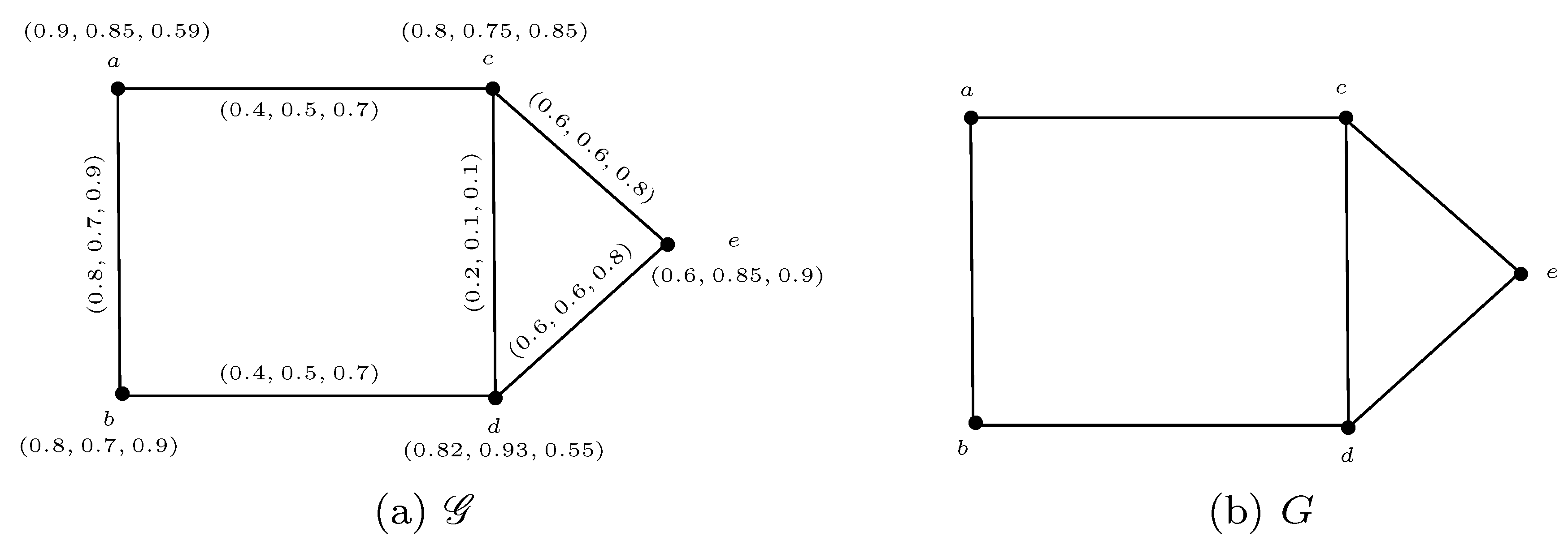
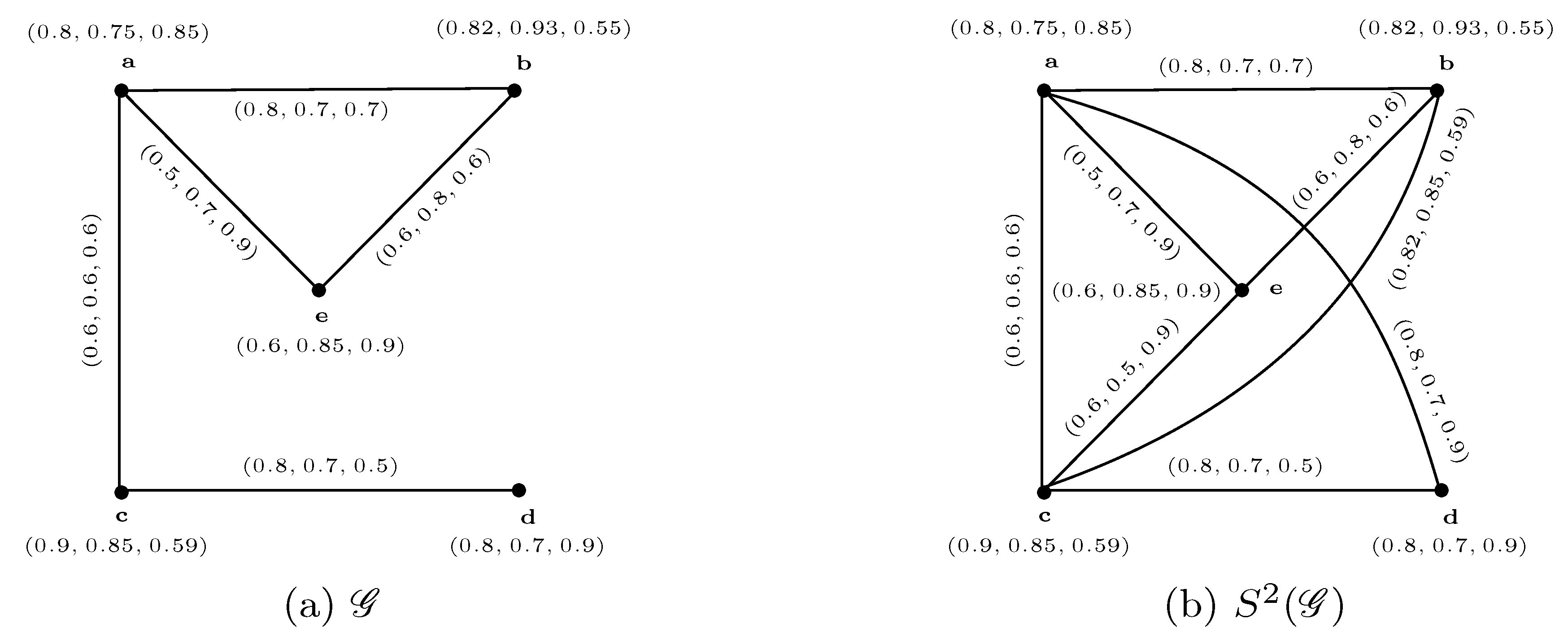
Example 15. 

Consider a 6-RPFG $\mathcal{G}=(\mathcal{P},\mathcal{Q})$ defined on $G=(P,Q),$ where $\mathcal{P}$ is a 6-rung picture fuzzy set on $P,$ and $\mathcal{Q}$ is a 6-rung picture fuzzy relation on $P,$ defined by

$\mathcal{P}$	a	b	c	d	e		$\mathcal{Q}$	$ab$	$ac$	$ae$	$cd$	$be$
${\mu }_{\mathcal{P}}$	0.8	0.82	0.9	0.8	0.6		${\mu }_{\mathcal{Q}}$	0.8	0.6	0.5	0.8	0.6
${\eta }_{\mathcal{P}}$	0.75	0.93	0.85	0.7	0.85		${\eta }_{\mathcal{Q}}$	0.7	0.6	0.7	0.7	0.8
${\nu }_{\mathcal{P}}$	0.85	0.55	0.59	0.9	0.9		${\nu }_{\mathcal{Q}}$	0.7	0.6	0.9	0.5	0.6

By routine computations, it is easy to see that $S^2(\mathcal{G})=(\mathcal{P},{\mathcal{Q}}_{sq})$ in Figure 15b is a square 6-rung picture fuzzy graph of $\mathcal{G},$ where the 6-rung picture fuzzy relation ${\mathcal{Q}}_{sq}$ can be defined as follows:

${\mathcal{Q}}_{sq}$	$ab$	$ac$	$ae$	$cd$	$be$	$ce$	$ad$	$bc$
${\mu }_{\mathcal{Q}}$	0.8	0.6	0.5	0.8	0.6	0.6	0.8	0.82
${\eta }_{\mathcal{Q}}$	0.7	0.6	0.7	0.7	0.8	0.5	0.7	0.85
${\nu }_{\mathcal{Q}}$	0.7	0.6	0.9	0.5	0.6	0.9	0.9	0.59

The following theorem defines the degree of an edge in square q-RPFG.

Theorem 20. 

For any q-RPFG $\mathcal{G}=(\mathcal{P},\mathcal{Q}),$ the degree of an edge in its square q-RPFG $S^2(\mathcal{G})=(\mathcal{P},{\mathcal{Q}}_{sq})$ is given by

1. 

For $uv\in Q,$

$$\begin{array}{cc}\hfill d_{S^2(\mathcal{G})}(uv)& =d_{\mathcal{G}}(uv)+\sum _{\begin{array}{c}ux\notin Q\\ ux\in Q_{sq}\end{array}}({\mu }_{\mathcal{P}}(u)\wedge {\mu }_{\mathcal{P}}(x),{\eta }_{\mathcal{P}}(u)\wedge {\eta }_{\mathcal{P}}(x),{\nu }_{\mathcal{P}}(u)\vee {\nu }_{\mathcal{P}}(x))+\hfill \\ & \sum _{\begin{array}{c}vy\notin Q\\ vy\in Q_{sq}\end{array}}({\mu }_{\mathcal{P}}(v)\wedge {\mu }_{\mathcal{P}}(y),{\eta }_{\mathcal{P}}(v)\wedge {\eta }_{\mathcal{P}}(y),{\nu }_{\mathcal{P}}(v)\vee {\nu }_{\mathcal{P}}(y)).\hfill \end{array}$$

2. 

For $uv\in Q_{sq}$ such that $uv\notin Q$,

$$\begin{array}{cc}\hfill d_{S^2(\mathcal{G})}(uv)& =d_{\mathcal{G}}(u)+d_{\mathcal{G}}(v)+\sum _{\begin{array}{c}ux\notin Q\\ ux\in Q_{sq}\end{array}}({\mu }_{\mathcal{P}}(u)\wedge {\mu }_{\mathcal{P}}(x),{\eta }_{\mathcal{P}}(u)\wedge {\eta }_{\mathcal{P}}(x),{\nu }_{\mathcal{P}}(u)\vee {\nu }_{\mathcal{P}}(x))+\hfill \\ & \sum _{\begin{array}{c}vy\notin Q\\ vy\in Q_{sq}\end{array}}({\mu }_{\mathcal{P}}(v)\wedge {\mu }_{\mathcal{P}}(y),{\eta }_{\mathcal{P}}(v)\wedge {\eta }_{\mathcal{P}}(y),{\nu }_{\mathcal{P}}(v)\vee {\nu }_{\mathcal{P}}(y))-2({\mu }_{{\mathcal{Q}}_{sq}}(uv),{\eta }_{{\mathcal{Q}}_{sq}}(uv),{\nu }_{{\mathcal{Q}}_{sq}}(uv)).\hfill \end{array}$$

Proof. 

Assume that $S^2(\mathcal{G})=(\mathcal{P},{\mathcal{Q}}_{sq})$ is a square q-RPFG of $\mathcal{G}=(\mathcal{P},\mathcal{Q}).$

1.

If $uv\in Q,$ then by definition of square q-RPFG $uv\in Q_{sq}.$ The degree of edge $uv$ in $S^2(\mathcal{G})$ is

$$\begin{array}{c}\hfill \begin{array}{cc}\hfill d_{S^2(\mathcal{G})}(uv)& =d_{S^2(\mathcal{G})}(u)+d_{S^2(\mathcal{G})}(v)-2({\mu }_{{\mathcal{Q}}_{sq}}(uv),{\eta }_{{\mathcal{Q}}_{sq}}(uv),{\nu }_{{\mathcal{Q}}_{sq}}(uv))\hfill \\ & =d_{\mathcal{G}}(u)+\sum _{\begin{array}{c}ux\notin Q\\ ux\in Q_{sq}\end{array}}({\mu }_{{\mathcal{Q}}_{sq}}(ux),{\eta }_{{\mathcal{Q}}_{sq}}(ux),{\nu }_{{\mathcal{Q}}_{sq}}(ux))+d_{\mathcal{G}}(v)+\sum _{\begin{array}{c}vy\notin Q\\ vy\in Q_{sq}\end{array}}({\mu }_{{\mathcal{Q}}_{sq}}(vy),{\eta }_{{\mathcal{Q}}_{sq}}(vy),\hfill \\ & {\nu }_{{\mathcal{Q}}_{sq}}(vy))-2({\mu }_{{\mathcal{Q}}_{sq}}(uv),{\eta }_{{\mathcal{Q}}_{sq}}(uv),{\nu }_{{\mathcal{Q}}_{sq}}(uv))\hfill \\ & =d_{\mathcal{G}}(u)+d_{\mathcal{G}}(v)-2({\mu }_{\mathcal{Q}}(uv),{\eta }_{\mathcal{Q}}(uv),{\nu }_{\mathcal{Q}}(uv)))+\sum _{\begin{array}{c}ux\notin Q\\ ux\in Q_{sq}\end{array}}({\mu }_{\mathcal{P}}(u)\wedge {\mu }_{\mathcal{P}}(x),{\eta }_{\mathcal{P}}(u)\wedge {\eta }_{\mathcal{P}}(x),\hfill \\ & {\nu }_{\mathcal{P}}(u)\vee {\nu }_{\mathcal{P}}(x))+\sum _{\begin{array}{c}vy\notin Q\\ vy\in Q_{sq}\end{array}}({\mu }_{\mathcal{P}}(v)\wedge {\mu }_{\mathcal{P}}(y),{\eta }_{\mathcal{P}}(v)\wedge {\eta }_{\mathcal{P}}(y),{\nu }_{\mathcal{P}}(v)\vee {\nu }_{\mathcal{P}}(y))\hfill \\ & =d_{\mathcal{G}}(uv)+\sum _{\begin{array}{c}ux\notin Q\\ ux\in Q_{sq}\end{array}}({\mu }_{\mathcal{P}}(u)\wedge {\mu }_{\mathcal{P}}(x),{\eta }_{\mathcal{P}}(u)\wedge {\eta }_{\mathcal{P}}(x),{\nu }_{\mathcal{P}}(u)\vee {\nu }_{\mathcal{P}}(x))+\hfill \\ & \sum _{\begin{array}{c}vy\notin Q\\ vy\in Q_{sq}\end{array}}({\mu }_{\mathcal{P}}(v)\wedge {\mu }_{\mathcal{P}}(y),{\eta }_{\mathcal{P}}(v)\wedge {\eta }_{\mathcal{P}}(y),{\nu }_{\mathcal{P}}(v)\vee {\nu }_{\mathcal{P}}(y)).\hfill \end{array}\end{array}$$

2.

If $uv\in Q_{sq}$ such that $uv\notin Q,$ then degree of edge $uv$ in $S^2(\mathcal{G})$ is

$$\begin{array}{c}\hfill \begin{array}{cc}\hfill d_{S^2(\mathcal{G})}(uv)& =d_{S^2(\mathcal{G})}(u)+d_{S^2(\mathcal{G})}(v)-2({\mu }_{{\mathcal{Q}}_{sq}}(uv),{\eta }_{{\mathcal{Q}}_{sq}}(uv),{\nu }_{{\mathcal{Q}}_{sq}}(uv))\hfill \\ & =d_{\mathcal{G}}(u)+\sum _{\begin{array}{c}ux\notin Q\\ ux\in Q_{sq}\end{array}}({\mu }_{{\mathcal{Q}}_{sq}}(ux),{\eta }_{{\mathcal{Q}}_{sq}}(ux),{\nu }_{{\mathcal{Q}}_{sq}}(ux))+d_{\mathcal{G}}(v)+\sum _{\begin{array}{c}vy\notin Q\\ vy\in Q_{sq}\end{array}}({\mu }_{{\mathcal{Q}}_{sq}}(vy),{\eta }_{{\mathcal{Q}}_{sq}}(vy),\hfill \\ & {\nu }_{{\mathcal{Q}}_{sq}}(vy))-2({\mu }_{{\mathcal{Q}}_{sq}}(uv),{\eta }_{{\mathcal{Q}}_{sq}}(uv),{\nu }_{{\mathcal{Q}}_{sq}}(uv))\hfill \\ & =d_{\mathcal{G}}(u)+d_{\mathcal{G}}(v)+\sum _{\begin{array}{c}ux\notin Q\\ ux\in Q_{sq}\end{array}}({\mu }_{\mathcal{P}}(u)\wedge {\mu }_{\mathcal{P}}(x),{\eta }_{\mathcal{P}}(u)\wedge {\eta }_{\mathcal{P}}(x),{\nu }_{\mathcal{P}}(u)\vee {\nu }_{\mathcal{P}}(x))+\hfill \\ & \sum _{\begin{array}{c}vy\notin Q\\ vy\in Q_{sq}\end{array}}({\mu }_{\mathcal{P}}(v)\wedge {\mu }_{\mathcal{P}}(y),{\eta }_{\mathcal{P}}(v)\wedge {\eta }_{\mathcal{P}}(y),{\nu }_{\mathcal{P}}(v)\vee {\nu }_{\mathcal{P}}(y))-2({\mu }_{{\mathcal{Q}}_{sq}}(uv),{\eta }_{{\mathcal{Q}}_{sq}}(uv),{\nu }_{{\mathcal{Q}}_{sq}}(uv)).\hfill \end{array}\end{array}$$

This completes the proof. □

Remark 8. 

If $\mathcal{G}=(\mathcal{P},\mathcal{Q})$ is edge regular q-RPFG, then $S^2(\mathcal{G})=(\mathcal{P},{\mathcal{Q}}_{sq})$ may not be edge regular.

For example, consider a 3-RPFG $\mathcal{G},$ and its square graph $S^2(\mathcal{G})$ as shown in Figure 16.

We see that $\mathcal{G}$ is $(1.0,0.6,1.2)$-edge regular 3-RPFG. However, since $d_{S^2(\mathcal{G})}(ab)=(2.3,1.4,2.7)\ne (2.0,1.2,2.4)=d_{S^2(\mathcal{G})}(ad).$ Hence, $S^2(\mathcal{G})$ is not edge regular.

Remark 9. 

If $S^2(\mathcal{G})=(\mathcal{P},{\mathcal{Q}}_{sq})$ is edge regular q-RPFG, then $\mathcal{G}=(\mathcal{P},\mathcal{Q})$ may not be edge regular.

For example, consider a 5-RPFG $\mathcal{G},$ and its square graph $S^2(\mathcal{G})$ as shown in Figure 17.

We see that $S^2(\mathcal{G})$ is $(2.0,2.4,2.8)$-edge regular 5-RPFG. However, since $d_{\mathcal{G}}(ab)=(1.5,1.8,2.1)\ne (2.0,2.4,2.8)=d_{\mathcal{G}}(ad).$ Hence, $\mathcal{G}$ is not edge regular.

Lemma 1. 

The square q-RPFG $S^2(\mathcal{G})$ of a complete q-RPFG $\mathcal{G}$ is the q-RPFG $\mathcal{G}$ itself.

Proof. 

The proof is obvious. □

Theorem 21. 

If $\mathcal{G}=(\mathcal{P},\mathcal{Q})$ be complete q-RPFG. Then, $\mathcal{G}$ is an edge regular q-RPFG if and only if $S^2(\mathcal{G})=(\mathcal{P},{\mathcal{Q}}_{sq})$ is an edge regular q-RPFG.

Proof. 

Let $\mathcal{G}=(\mathcal{P},\mathcal{Q})$ be complete q-RPFG. By Lemma 1, $\mathcal{G},$ and $S^2(\mathcal{G})$ are same. It follows that $\mathcal{G}$ is an edge regular q-RPFG if and only if $S^2(\mathcal{G})=(\mathcal{P},{\mathcal{Q}}_{sq})$ is an edge regular q-RPFG. □

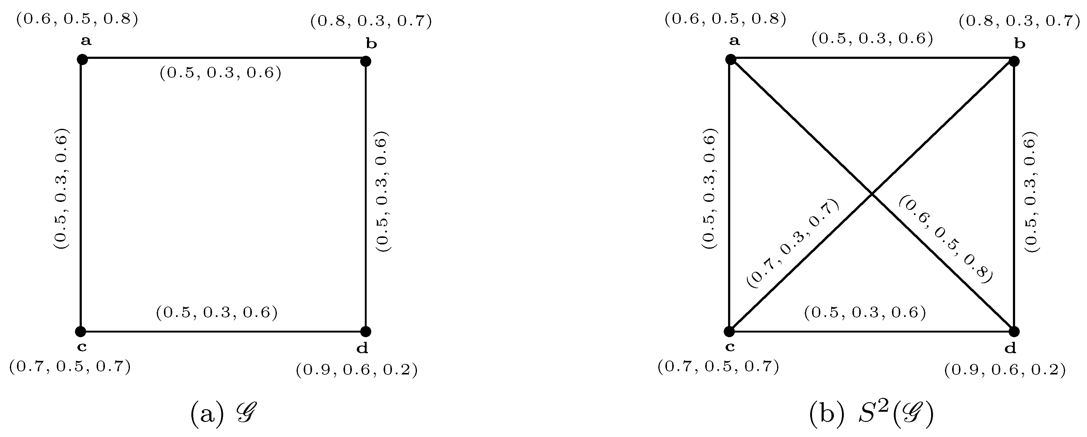
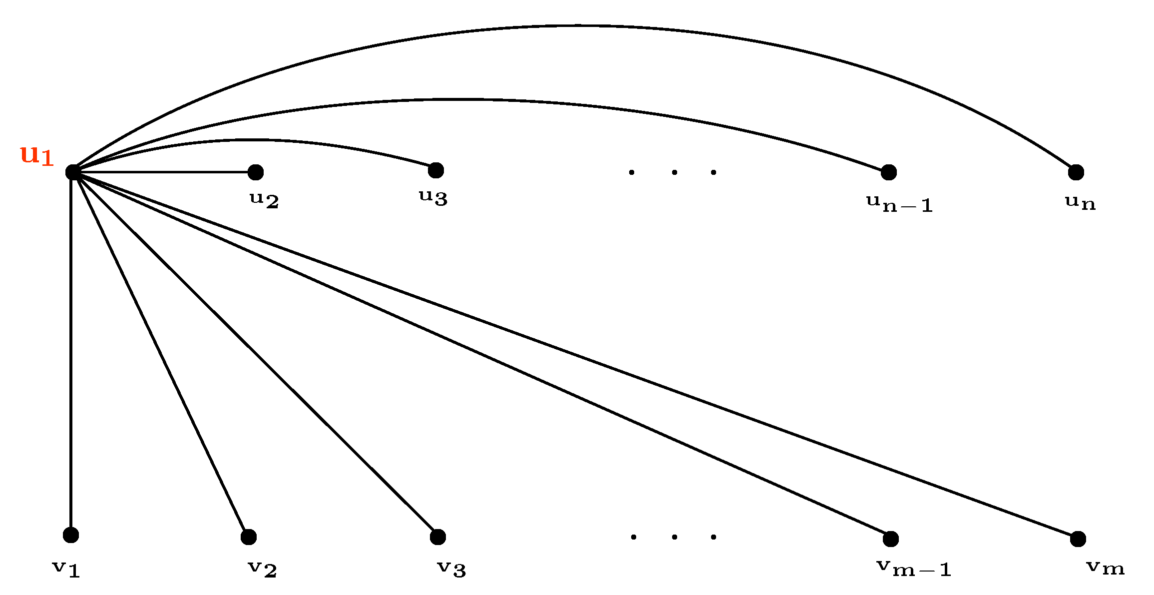
Lemma 2. 

The square q-RPFG $S^2(\mathcal{G})$ of a complete bipartite q-RPFG $\mathcal{G}$ is complete.

Proof. 

Let $\mathcal{G}=(\mathcal{P},\mathcal{Q})$ be a q-RPFG defined on a complete bipartite graph $G=(P,Q).$ Then, ${\mu }_{\mathcal{Q}}(u_i{v}_j)={\mu }_{\mathcal{P}}(u_i)\wedge {\mu }_{\mathcal{P}}(v_j),{\eta }_{\mathcal{Q}}(u_i{v}_j)={\eta }_{\mathcal{P}}(u_i)\wedge {\eta }_{\mathcal{P}}(v_j),$ and ${\nu }_{\mathcal{Q}}(u_i{v}_j)={\nu }_{\mathcal{P}}(u_i)\wedge {\nu }_{\mathcal{P}}(v_j)$ for all $u_i\in P_1,$ and $v_j\in P_2,$ where $P=P_1\cup P_2.$ Let $S^2(\mathcal{G})=(\mathcal{P},{\mathcal{Q}}_{sq})$ be the square q-RPFG of $\mathcal{G}.$ Then, we have the following:

• If $u_i{v}_j\in Q,$ then ${\mu }_{{\mathcal{Q}}_{sq}}(u_i{v}_j)={\mu }_{\mathcal{Q}}(u_i{v}_j),{\eta }_{{\mathcal{Q}}_{sq}}(u_i{v}_j)={\eta }_{\mathcal{Q}}(u_i{v}_j),$ and ${\nu }_{{\mathcal{Q}}_{sq}}(u_i{v}_j)={\nu }_{\mathcal{Q}}(u_i{v}_j).$
• If $u_i{v}_j\notin Q,$ and $u,v$ are joined by a path of length less then or equal to 2 in $G,$ then ${\mu }_{{\mathcal{Q}}_{sq}}(u_i{v}_j)\le {\mu }_{\mathcal{P}}(u_i)\wedge {\mu }_{\mathcal{P}}(v_j),{\eta }_{{\mathcal{Q}}_{sq}}(u_i{v}_j)\le {\eta }_{\mathcal{P}}(u_i)\wedge {\eta }_{\mathcal{P}}(v_j),$ and ${\nu }_{{\mathcal{Q}}_{sq}}(u_i{v}_j)\le {\nu }_{\mathcal{P}}(u_i)\vee {\nu }_{\mathcal{P}}(v_j).$

Since each pair of vertices in a complete bipartite graph must connected by a path of length less then or equal to 2 (see Figure 18), therefore, above axioms imply that for all $u_i,v_j\in P$

$$\begin{array}{ccc}\hfill {\mu }_{{\mathcal{Q}}_{sq}}(u_i{v}_j)& \le & {\mu }_{\mathcal{P}}(u_i)\wedge {\mu }_{\mathcal{P}}(v_j),\hfill \\ \hfill {\eta }_{{\mathcal{Q}}_{sq}}(u_i{v}_j)& \le & {\eta }_{\mathcal{P}}(u_i)\wedge {\eta }_{\mathcal{P}}(v_j),\hfill \\ \hfill {\nu }_{{\mathcal{Q}}_{sq}}(u_i{v}_j)& \le & {\nu }_{\mathcal{P}}(u_i)\vee {\nu }_{\mathcal{P}}(v_j).\hfill \end{array}$$

Hence, the square q-RPFG $S^2(\mathcal{G})$ is complete. This completes the proof. □

Theorem 22. 

If $\mathcal{G}=(\mathcal{P},\mathcal{Q})$ is a complete bipartite q-RPFG such that ${\mu }_{\mathcal{P}},{\eta }_{\mathcal{P}},$ and ${\nu }_{\mathcal{P}}$ are constant functions, then its square graph $S^2(\mathcal{G})$ is edge regular.

Proof. 

Let $\mathcal{G}=(\mathcal{P},\mathcal{Q})$ be a complete bipartite q-RPFG such that ${\mu }_{\mathcal{P}},{\eta }_{\mathcal{P}},$ and ${\nu }_{\mathcal{P}}$ are constant functions. Assume that $S^2(\mathcal{G})=(\mathcal{P},{\mathcal{Q}}_{sq})$ is the square q-RPFG of $\mathcal{G}.$ Then, by Lemma 2, $S^2(\mathcal{G})$ is a complete q-RPFG.

Let ${\mu }_{\mathcal{P}}(u)=c_1,{\eta }_{\mathcal{P}}(u)=c_2,$ and ${\nu }_{\mathcal{P}}(u)=c_3$ for all $u\in P.$ By definition of square q-RPFG, we have

$$\begin{array}{ccc}\hfill {\mu }_{{\mathcal{Q}}_{sq}}(uv)& \le & {\mu }_{\mathcal{P}}(u)\wedge {\mu }_{\mathcal{P}}(v)=c_1\wedge c_1=c_1,\hfill \\ \hfill {\eta }_{{\mathcal{Q}}_{sq}}(uv)& \le & {\eta }_{\mathcal{P}}(u)\wedge {\eta }_{\mathcal{P}}(v)=c_2\wedge c_2=c_2,\hfill \\ \hfill {\nu }_{{\mathcal{Q}}_{sq}}(uv)& \le & {\nu }_{\mathcal{P}}(u)\vee {\nu }_{\mathcal{P}}(v)=c_3\vee c_3=c_3.\hfill \end{array}$$

Hence, ${\mu }_{{\mathcal{Q}}_{sq}},{\eta }_{{\mathcal{Q}}_{sq}},$ and ${\nu }_{{\mathcal{Q}}_{sq}}$ are constant functions. Thus, by Theorem 8, $S^2(\mathcal{G})$ is edge regular. This completes the proof. □

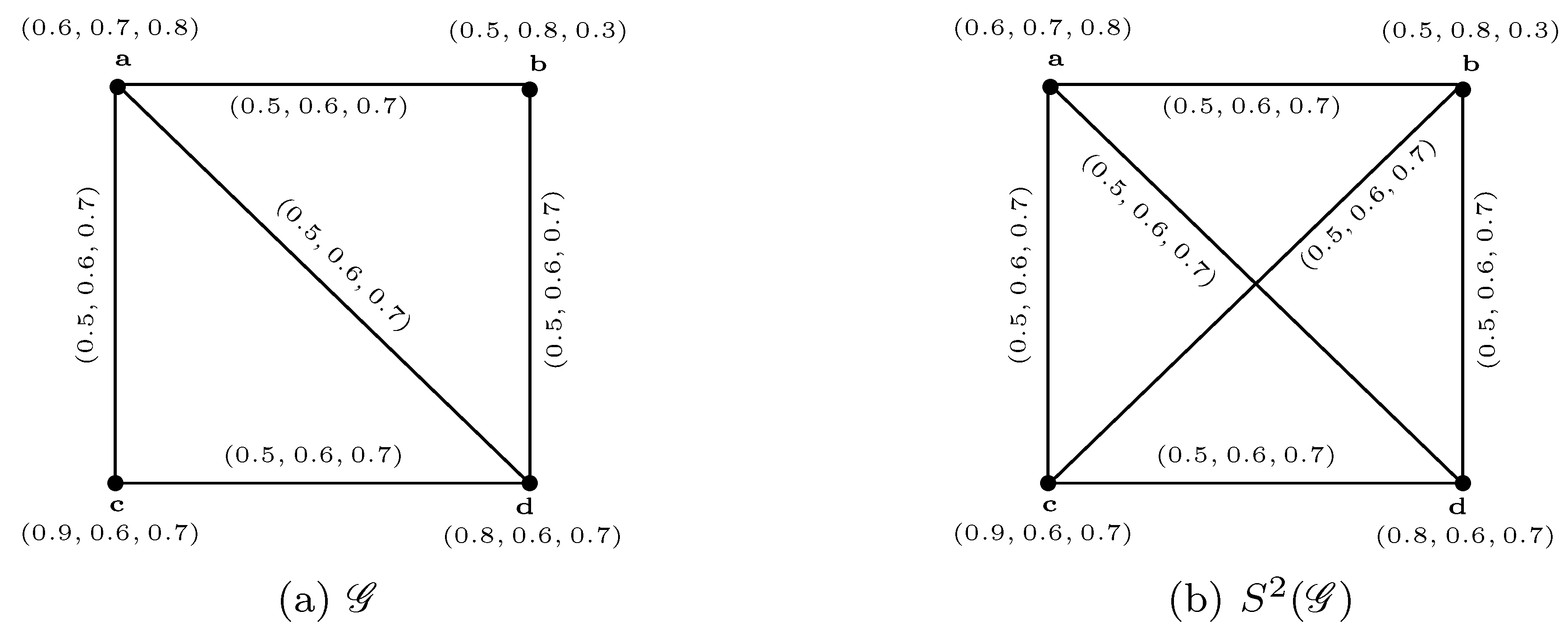
Theorem 23. 

If $\mathcal{G}$ is a q-RPFG on a cycle of length n such that ${\mu }_{\mathcal{Q}},{\eta }_{\mathcal{Q}},$ and ${\nu }_{\mathcal{Q}}$ are constant functions, then its square q-RPFG $S^2(\mathcal{G})$ is edge regular.

Proof. 

Let $\mathcal{G}=(\mathcal{P},\mathcal{Q})$ be a q-RPFG defined on a cycle $u_1{u}_2{u}_3\dots u_{n-1}{u}_n{u}_1$ (see Figure 19). Assume that ${\mu }_{\mathcal{Q}},{\eta }_{\mathcal{Q}},$ and ${\nu }_{\mathcal{Q}}$ are constant functions, and ${\mu }_{\mathcal{Q}}(u_i{u}_{i+1})=c_1,{\eta }_{\mathcal{Q}}(u_i{u}_{i+1})=c_2,$ and ${\nu }_{\mathcal{Q}}(u_i{u}_{i+1})=c_3$ for all $i=1,2,\dots ,n,$ where $n+1=1.$ The degree of edge $u_i{u}_{i+1}$ can be computed as:

$$\begin{array}{c}\hfill \begin{array}{cc}\hfill d_{\mathcal{G}}(u_i{u}_{i+1})& =d_{\mathcal{G}}(u_i)+d_{\mathcal{G}}(u_{i+1})-2({\mu }_{\mathcal{Q}}(u_i{u}_{i+1}),{\eta }_{\mathcal{Q}}(u_i{u}_{i+1}),{\nu }_{\mathcal{Q}}(u_i{u}_{i+1}))\hfill \\ & =({\mu }_{\mathcal{Q}}(u_{i-1}{u}_i),{\eta }_{\mathcal{Q}}(u_{i-1}{u}_i),{\nu }_{\mathcal{Q}}(u_{i-1}{u}_i))+2({\mu }_{\mathcal{Q}}(u_i{u}_{i+1}),{\eta }_{\mathcal{Q}}(u_i{u}_{i+1}),{\nu }_{\mathcal{Q}}(u_i{u}_{i+1}))+\hfill \\ & ({\mu }_{\mathcal{Q}}(u_{i+1}{u}_{i+2}),{\eta }_{\mathcal{Q}}(u_{i+1}{u}_{i+2}),{\nu }_{\mathcal{Q}}(u_{i+1}{u}_{i+2}))-2({\mu }_{\mathcal{Q}}(u_i{u}_{i+1}),{\eta }_{\mathcal{Q}}(u_i{u}_{i+1}),{\nu }_{\mathcal{Q}}(u_i{u}_{i+1}))\hfill \\ & =({\mu }_{\mathcal{Q}}(u_{i-1}{u}_i),{\eta }_{\mathcal{Q}}(u_{i-1}{u}_i),{\nu }_{\mathcal{Q}}(u_{i-1}{u}_i))+({\mu }_{\mathcal{Q}}(u_{i+1}{u}_{i+2}),{\eta }_{\mathcal{Q}}(u_{i+1}{u}_{i+2}),{\nu }_{\mathcal{Q}}(u_{i+1}{u}_{i+2}))\hfill \\ & =(c_1,c_2,c_3)+(c_1,c_2,c_3)=2(c_1,c_2,c_3).\hfill \end{array}\end{array}$$

Hence, $\mathcal{G}$ is edge regular. Let $S^2(\mathcal{G})$ be the square q-RPFG of $\mathcal{G}.$ To prove that $S^2(\mathcal{G})$ is edge regular, there arise three cases:

Case-I When $n=3,$ we have a complete q-RPFG $\mathcal{G}.$ By Lemma 1, $S^2(\mathcal{G})$ is $\mathcal{G}$ itself.

Case-II When $n=4,$ each pair of non-adjacent vertices is connected by two distinct paths of length 2. Thus, its square graph $S^2(\mathcal{G})$ will be a complete q-RPFG with ${\mu }_{\mathcal{Q}},{\eta }_{\mathcal{Q}},$ and ${\nu }_{\mathcal{Q}}$ are constant functions. In this case, $S^2(\mathcal{G})$ is edge regular by Theorem 8.

Case-III Let $n\ge 5.$ Consider a vertex u in $S^2(\mathcal{G}).$ There are exactly two vertices which are at distance 2 from $u.$ Therefore, u is adjacent to exactly two more vertices in $S^2(\mathcal{G}).$ Hence, $S^2(\mathcal{G})$ is 4-regular. Then, for each $uv$ in $S^2(\mathcal{G}),$ we have

$$\begin{array}{ccc}\hfill d_{S^2(\mathcal{G})}(uv)& =& d_{S^2(\mathcal{G})}(u)+d_{S^2(\mathcal{G})}(v)-2({\mu }_{{\mathcal{Q}}_{sq}}(uv),{\eta }_{{\mathcal{Q}}_{sq}}(uv),{\nu }_{{\mathcal{Q}}_{sq}}(uv))\hfill \\ & =& 4(c_1,c_2,c_3)+4(c_1,c_2,c_3)-2(c_1,c_2,c_3)=6(c_1,c_2,c_3).\hfill \end{array}$$

Hence, $S^2(\mathcal{G})$ is $6(c_1,c_2,c_3)$-edge regular. This completes the proof. □

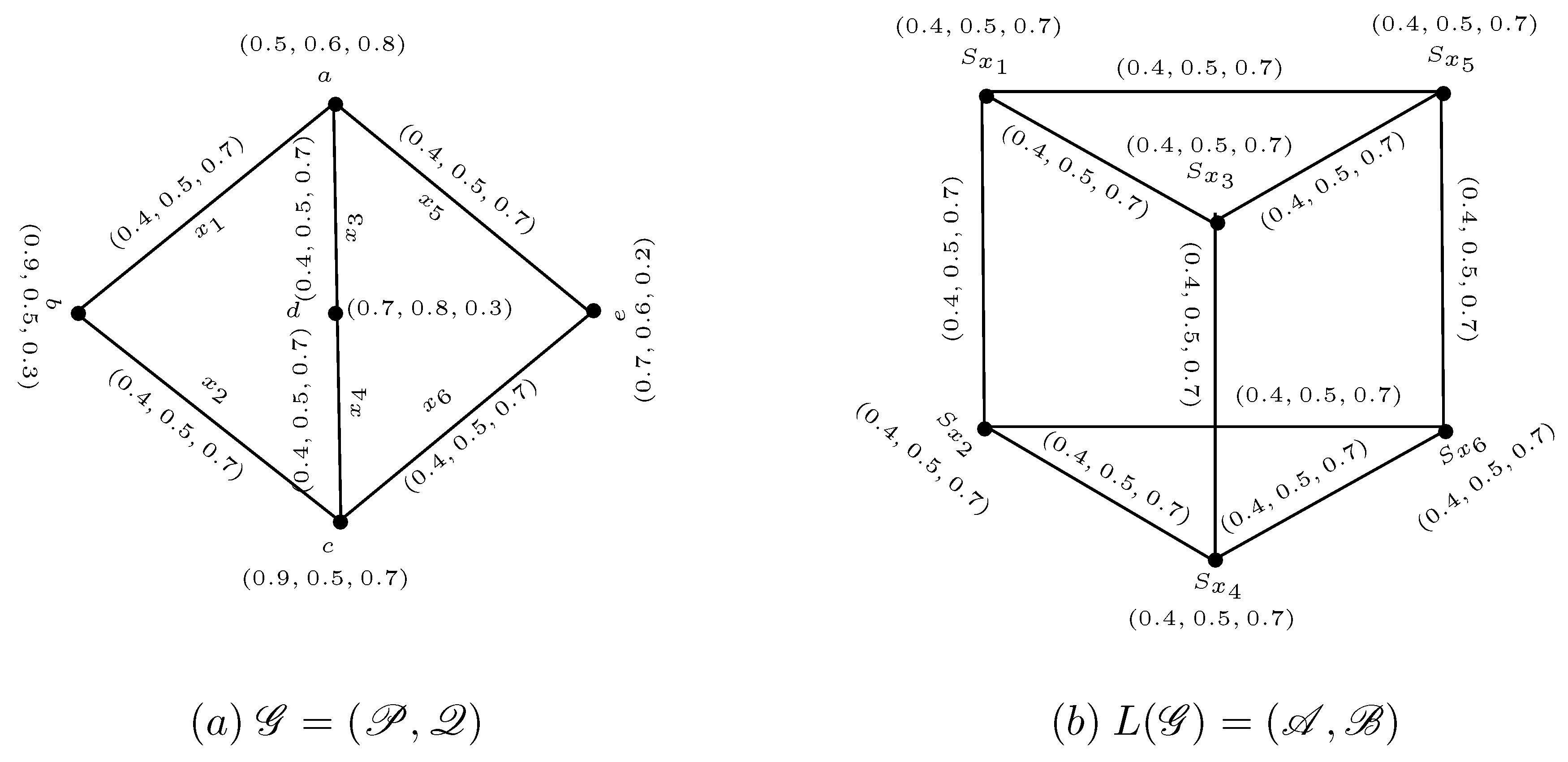
2.3. Edge Regular q-RPF Line Graphs

Following [45], this section gives a brief discussion on edge regular q-rung picture fuzzy line graphs (q-RPFLGs). Akram and Habib [35] defined the q-RPFLGs as follows:

Definition 24. 

Let $\mathcal{G}=(\mathcal{P},\mathcal{Q})$ be a q-RPFG defined on $G=(P,Q).$ The q-rung picture fuzzy line graph $L(\mathcal{G})=(\mathcal{A},\mathcal{B})$ with underlying graph $L(G)=(A,B)$ where $A=\{S_x=\left\{x\right\}\cup \left\{u_x{v}_x\right\}|x\in Q,x=u_x{v}_x,u_x,v_x\in P\}$ and $B=\left\{S_x{S}_y\right|S_x\cap S_y\ne \varphi ,x,y\in Q,x\ne y\}$ can be defined as

(i)

For each vertex $S_x$ in $A,$

$${\mu }_{\mathcal{A}}(S_x)={\mu }_{\mathcal{Q}}(x),{\eta }_{\mathcal{A}}(S_x)={\eta }_{\mathcal{Q}}(x),{\nu }_{\mathcal{A}}(S_x)={\nu }_{\mathcal{Q}}(x).$$

(ii)

For each edge $S_x{S}_y$ in $B,$

$$\begin{array}{ccc}\hfill {\mu }_{\mathcal{B}}(S_x{S}_y)& =& min\{{\mu }_{\mathcal{A}}(S_x),{\mu }_{\mathcal{A}}(S_y)\},\hfill \\ \hfill {\eta }_{\mathcal{B}}(S_x{S}_y)& =& min\{{\eta }_{\mathcal{A}}(S_x),{\eta }_{\mathcal{A}}(S_y)\},\hfill \\ \hfill {\nu }_{\mathcal{B}}(S_x{S}_y)& =& max\{{\nu }_{\mathcal{A}}(S_x),{\nu }_{\mathcal{A}}(S_y)\}.\hfill \end{array}$$

Theorem 24. 

Let $\mathcal{G}=(\mathcal{P},\mathcal{Q})$ be a q-RPFG such that ${\mu }_{\mathcal{Q}},{\eta }_{\mathcal{Q}},$ and ${\nu }_{\mathcal{Q}}$ are constant functions. Then, $d_{L(\mathcal{G})}(S_x{S}_y)=(c_1,c_2,c_3)[d_{L(G)}(S_x)+d_{L(G)}(S_y)-2]$ for all $S_x{S}_y\in B.$

Proof. 

Let $L(\mathcal{G})=(\mathcal{A},\mathcal{B})$ be a q-rung picture fuzzy line graph of a q-RPFG $\mathcal{G}=(\mathcal{P},\mathcal{Q}).$ For any $S_x{S}_y\in B,$

$$\begin{array}{c}\hfill \begin{array}{cc}\hfill d_{L(\mathcal{G})}(S_x{S}_y)& =d_{L(\mathcal{G})}(S_x)+d_{L(\mathcal{G})}(S_y)-2({\mu }_{\mathcal{B}}(S_x{S}_y),{\eta }_{\mathcal{B}}(S_x{S}_y),{\nu }_{\mathcal{B}}(S_x{S}_y))\hfill \\ & =\sum _{S_x{S}_z\in B}({\mu }_{\mathcal{Q}}(S_x{S}_z),{\eta }_{\mathcal{Q}}(S_x{S}_z),{\nu }_{\mathcal{Q}}(S_x{S}_z))+\sum _{S_y{S}_z\in B}({\mu }_{\mathcal{Q}}(S_y{S}_z),{\eta }_{\mathcal{Q}}(S_y{S}_z),{\nu }_{\mathcal{Q}}(S_y{S}_z))\hfill \\ & -2({\mu }_{\mathcal{Q}}(S_x{S}_y),{\eta }_{\mathcal{Q}}(S_x{S}_y),{\nu }_{\mathcal{Q}}(S_x{S}_y))\hfill \\ & =(c_1,c_2,c_3)d_{L(G)}(S_x)+(c_1,c_2,c_3)d_{L(G)}(S_y)-2(c_1,c_2,c_3)\hfill \\ & =(c_1,c_2,c_3)[d_{L(G)}(S_x)+d_{L(G)}(S_y)-2].\hfill \end{array}\end{array}$$

This completes the proof. □

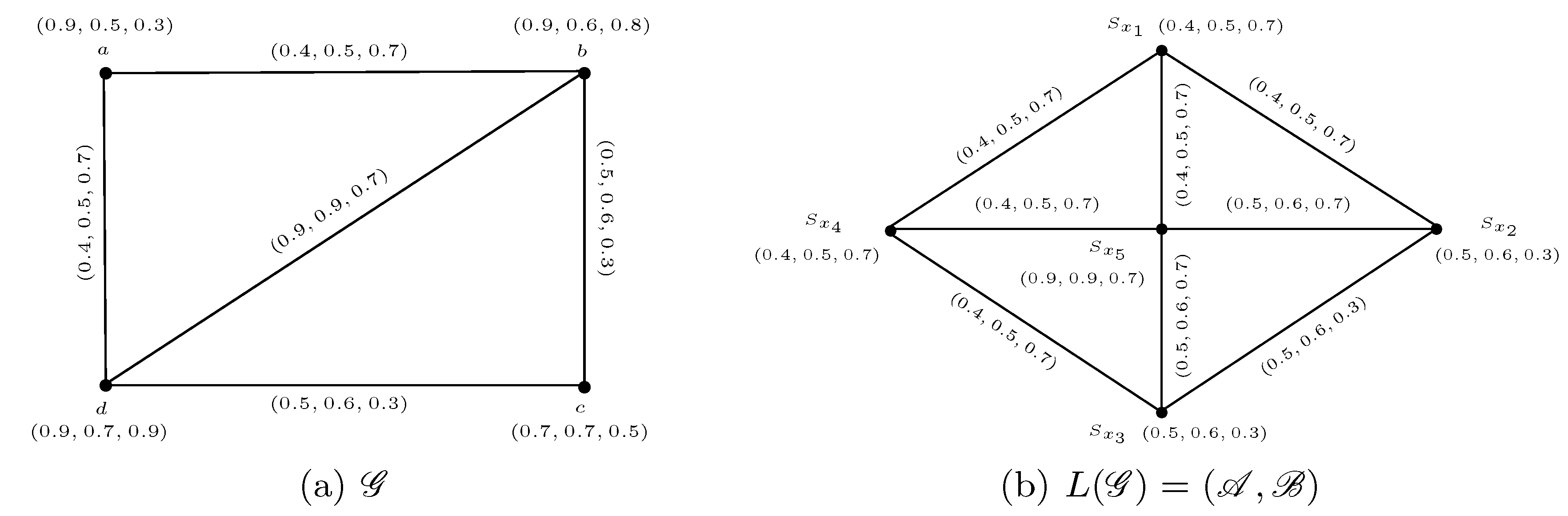
Remark 10. 

Consider a 6-RPFG $\mathcal{G}=(\mathcal{P},\mathcal{Q})$ as displayed in Figure 20a. Its corresponding line graph $L(\mathcal{G})=(\mathcal{A},\mathcal{B})$ is displayed in Figure 20b.

We see that $\mathcal{G}$ is $(1.8,1.8,1.4)$-edge regular 6-RPFG. However, since $d_{L(\mathcal{G})}(S_{x_1}{S}_{x_5})=(2.2,2.7,3.5)\ne (1.8,2.2,2.4)=d_{L(\mathcal{G})}(S_{x_1}{S}_{x_2});$ therefore, $L(\mathcal{G})$ is not an edge regular 6-RPFG.

We now develop a necessary condition for q-RPFLG to be perfect edge regular.

Theorem 25. 

Every q-rung picture fuzzy line graph $L(\mathcal{G})=(\mathcal{A},\mathcal{B})$ of an edge regular q-RPFG $\mathcal{G}=(\mathcal{P},\mathcal{Q})$ is perfect edge regular only if ${\mu }_{\mathcal{Q}},{\eta }_{\mathcal{Q}},$ and ${\nu }_{\mathcal{Q}}$ are constant functions in $\mathcal{G}.$

Proof. 

Let $\mathcal{G}=(\mathcal{P},\mathcal{Q})$ be an edge regular q-RPFG defined on $G=(P,Q).$ Then, for each edge $uv$ in $\mathcal{Q},d(uv)=(p_1,p_2,p_3).$ Let ${\mu }_{\mathcal{Q}},{\eta }_{\mathcal{Q}},$ and ${\nu }_{\mathcal{Q}}$ be constant functions. Then, for each edge $uv$ in $\mathcal{Q},{\mu }_{\mathcal{Q}}(uv)=c_1,{\eta }_{\mathcal{Q}}(uv)=c_2\mathrm{and}{\nu }_{\mathcal{Q}}(uv)=c_3.$ Consider $L(\mathcal{G})=(\mathcal{A},\mathcal{B})$ as a q-RPFG as a q-rung picture fuzzy line graph of $\mathcal{G}.$ Then, by definition of q-rung picture fuzzy line graph, each vertex $S_x$ of $L(\mathcal{G})$ corresponding to an edge $uv=x$ of $\mathcal{G}$ has membership value $({\mu }_{\mathcal{A}}(S_x),{\eta }_{\mathcal{A}}(S_x),{\nu }_{\mathcal{A}}(S_x))=({\mu }_{\mathcal{Q}}(uv),{\eta }_{\mathcal{Q}}(uv),{\nu }_{\mathcal{Q}}(uv))=(c_1,c_2,c_3),$ and each edge of $L(\mathcal{G})$ has membership value

$$\begin{array}{ccc}\hfill ({\mu }_{\mathcal{B}}(S_x{S}_y),{\eta }_{\mathcal{B}}(S_x{S}_y),{\nu }_{\mathcal{B}}(S_x{S}_y))& =& ({\mu }_{\mathcal{A}}(S_x)\wedge {\mu }_{\mathcal{A}}(S_y),{\eta }_{\mathcal{A}}(S_x)\wedge {\eta }_{\mathcal{A}}(S_y),{\eta }_{\mathcal{A}}(S_x)\vee {\eta }_{\mathcal{A}}(S_y))\hfill \\ & =& (c_1\wedge c_1,c_2\wedge c_2,c_3\vee c_3)\hfill \\ & =& (c_1,c_2,c_3).\hfill \end{array}$$

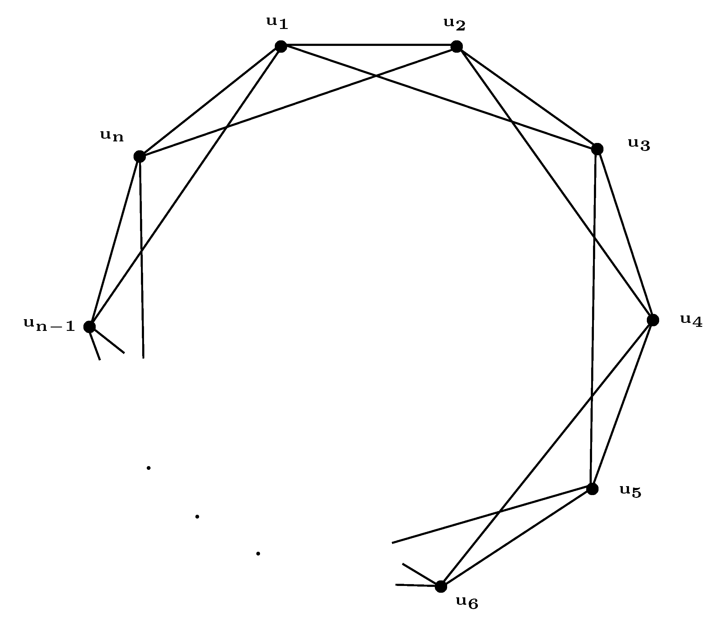
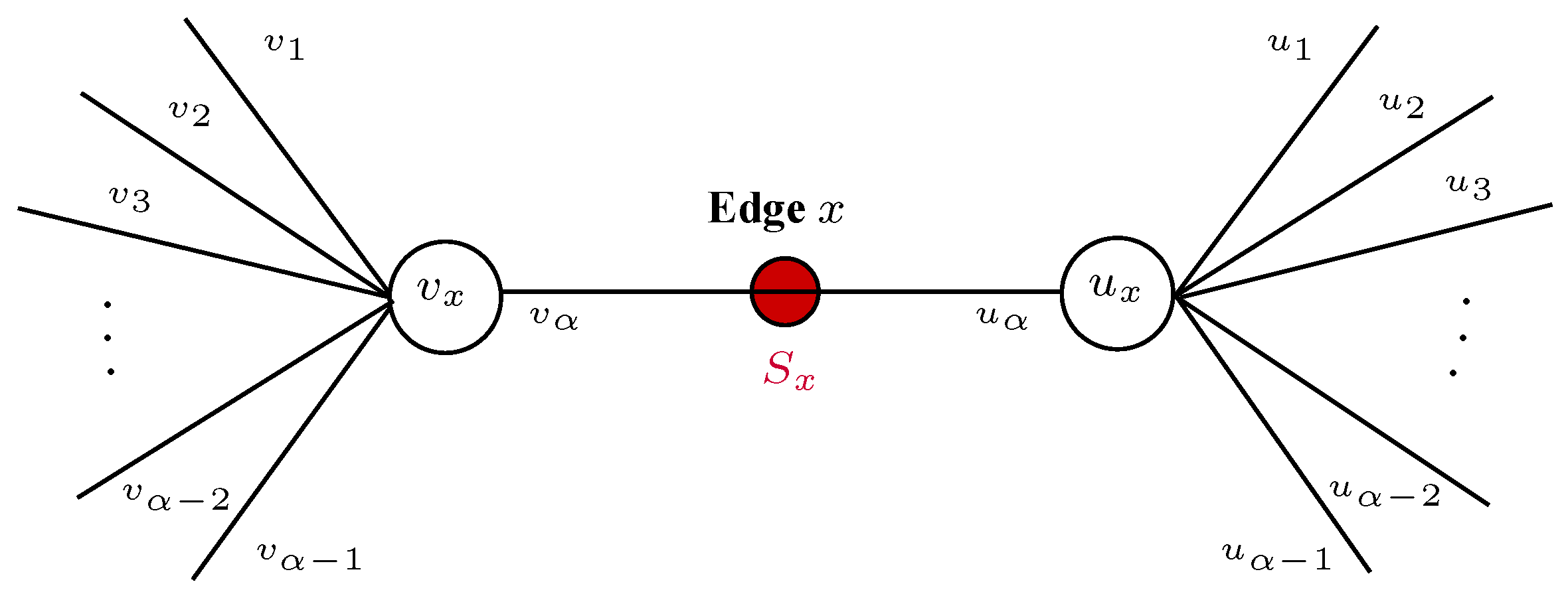
Let $u(x)$ and $v(x)$ be the end points of an edge $uv=x$ in $\mathcal{G}.$ Since $\mathcal{G}$ is edge regular with constant functions ${\mu }_{\mathcal{Q}},{\eta }_{\mathcal{Q}},$ and ${\nu }_{\mathcal{Q}},$ therefore, each vertex u of $\mathcal{G}$ is common vertex of α (say) edges in $\mathcal{G}$ (see Figure 21).

Let $S_x$ be the vertex of $L(\mathcal{G})$ corresponding to an edge x in $\mathcal{G}.$ The edge x has a vertex $v_x$ in common with $\alpha -1$ edges $v_1,v_2,\dots ,v_{\alpha -1}.$ Similarly, $u_x$ is common with $\alpha -1$ edges $u_1,u_2,\dots ,u_{\alpha -1}$ in $\mathcal{G}.$ Thus, each vertex $S_x$ in $L(\mathcal{G})$ is common vertex of $\alpha -1+\alpha -1=2\alpha -2$ edges. Hence, for all $S_x$ in $L(G)$

$$d_{L(G)}(S_x)=2\alpha -2.$$

(1)

By Theorem 24, we have $d_{L(\mathcal{G})}(S_x{S}_y)=(c_1,c_2,c_3)[d_{L(G)}(S_x)+d_{L(G)}(S_y)-2].$ Then, by Equation (1), $d_{L(\mathcal{G})}(S_x{S}_y)=(c_1,c_2,c_3)[2\alpha -2+2\alpha -2-2]=2(2\alpha -3)(c_1,c_2,c_3),$ which implies that $L(\mathcal{G})$ is an edge regular q-RPFG. Moreover, $t{d}_{L(\mathcal{G})}(S_x{S}_y)=d_{L(\mathcal{G})}(S_x{S}_y)+({\mu }_{\mathcal{B}}(S_x{S}_y),{\eta }_{\mathcal{B}}(S_x{S}_y),{\nu }_{\mathcal{B}}(S_x{S}_y))=2(2\alpha -3)(c_1,c_2,c_3)+(c_1,c_2,c_3)=(4\alpha -5)(c_1,c_2,c_3),$ which shows that $L(\mathcal{G})$ is total edge regular q-RPFG. Consequently, $L(\mathcal{G})$ is perfect edge regular q-RPFG. This completes the proof. □

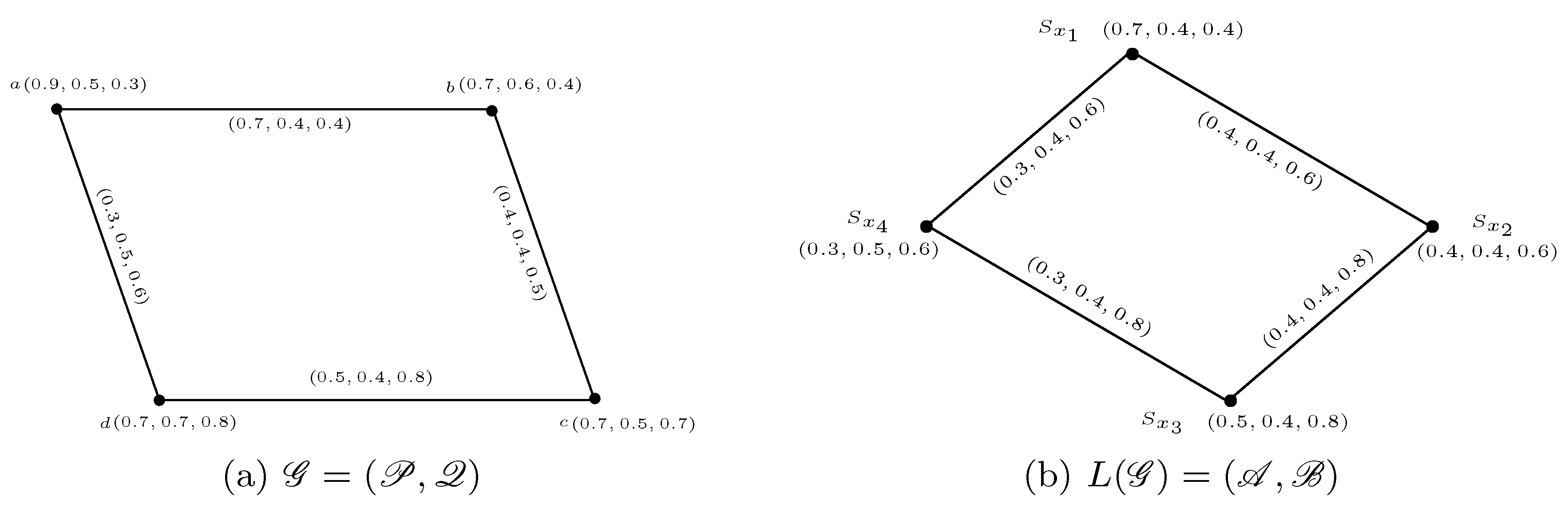
Remark 11. 

Consider a 4-RPFG $\mathcal{G}=(\mathcal{P},\mathcal{Q})$ as displayed in Figure 22a, and its line graph $L(\mathcal{G})=(\mathcal{A},\mathcal{B})$ Figure 22b.

We see that $L(\mathcal{G})$ is $(0.7,0.8,1.4)$-edge regular 4-RPFLG. However, since $d_{\mathcal{G}}(ab)=(0.7,0.7,1.1)\ne (1.2,0.8,1.2)=d_{\mathcal{G}}(bc);$ therefore, $\mathcal{G}$ is not an edge regular 4-RPFG.

Theorem 26. 

If $L(\mathcal{G})=(\mathcal{A},\mathcal{B})$ is an edge regular q-rung picture fuzzy line graph of $\mathcal{G}=(\mathcal{P},\mathcal{Q}),$ and ${\mu }_{\mathcal{Q}},{\eta }_{\mathcal{Q}},$ and ${\nu }_{\mathcal{Q}}$ are constant functions, then $\mathcal{G}$ is edge regular q-RPFG.

Proof. 

The proof is similar to the proof of Theorem 25. □

Theorem 27. 

Let $\mathcal{G}=(\mathcal{P},\mathcal{Q})$ be a strong q-rung picture fuzzy graph such that ${\mu }_{\mathcal{P}},{\eta }_{\mathcal{P}},$ and ${\nu }_{\mathcal{P}}$ are constant functions. If $\mathcal{G}$ is an edge regular q-RPFG, then its line graph $L(\mathcal{G})=(\mathcal{A},\mathcal{B})$ is an edge regular q-rung picture fuzzy graph.

Proof. 

Let $\mathcal{G}=(\mathcal{P},\mathcal{Q})$ be a strong edge regular q-rung picture fuzzy graph such that ${\mu }_{\mathcal{P}},{\eta }_{\mathcal{P}},$ and ${\nu }_{\mathcal{P}}$ are constant functions. Then, the functions ${\mu }_{\mathcal{Q}},{\eta }_{\mathcal{Q}},$ and ${\nu }_{\mathcal{Q}}$ must be constants. Consequently, the result follows from Theorem 25. □

3. Relations between Regular and Edge-Regular q-RPFGs

The fact that edge regularity property is a strong analog of regularity in fuzzy graphs is shown by many researchers. This section provides some additional properties relating regularity and edge regularity of q-RPFGs.

Remark 12. 

Every regular q-RPFG need not be edge regular.

For example, consider a 5-RPFG $\mathcal{G}=(\mathcal{P},\mathcal{Q})$ displayed in Figure 23.

It is clear that $\mathcal{G}$ is $(1.75,1.72,2.2)$-regular 5-RPFG, but $\mathcal{G}$ is not edge regular as $d_{\mathcal{G}}(ab)=(2.0,2.2,3.0)\ne (2.5,2.44,2.8)=d_{\mathcal{G}}(bc).$

Remark 13. 

Every edge regular q-RPFG need not be regular.

For example, consider a 6-RPFG $\mathcal{G}$ as shown in Figure 10. It is clear that $\mathcal{G}$ is $(1.4,1.8,1.6)$-edge regular 6-RPFG but $\mathcal{G}$ is not regular as $d_{\mathcal{G}}(u)=(0.8,1.0,0.6)\ne (1.4,1.8,1.6)=d_{\mathcal{G}}(v).$

The above remarks show that one form of regularity can not imply another form. We now develop some results between regularity and edge regularity.

Theorem 28. 

Let $\mathcal{G}=(\mathcal{P},\mathcal{Q})$ be a regular q-RPFG on $G=(P,Q).$ Then, $\mathcal{G}$ is edge regular if and only if ${\mu }_{\mathcal{Q}},{\eta }_{\mathcal{Q}},$ and ${\nu }_{\mathcal{Q}}$ are constant functions.

Proof. 

Let $\mathcal{G}=(\mathcal{P},\mathcal{Q})$ be a $(k_1,k_2,k_3)$-regular q-RPFG. Then, $d_{\mathcal{G}}(u)=(k_1,k_2,k_3)$ for all $u\in P.$ Assume that ${\mu }_{\mathcal{Q}},{\eta }_{\mathcal{Q}},$ and ${\nu }_{\mathcal{Q}}$ are constant functions, that is, ${\mu }_{\mathcal{Q}}(uv)=c_1,{\eta }_{\mathcal{Q}}(uv)=c_2,$ and ${\nu }_{\mathcal{Q}}(uv)=c_3.$ By definition of edge degree $d_{\mathcal{G}}(uv)=d_{\mathcal{G}}(u)+d_{\mathcal{G}}(v)-2({\mu }_{\mathcal{Q}}(uv),{\eta }_{\mathcal{Q}}(uv),{\nu }_{\mathcal{Q}}(uv))=2(k_1,k_2,k_3)-2(c_1,c_2,c_3)=2(p_1-c_1,p_2-c_2,p_3-c_3)$ for all $uv\in Q.$ Hence, $\mathcal{G}$ is edge regular.

Conversely, assume that $\mathcal{G}$ is $(p_1,p_2,p_3)$-edge regular. Then, $d_{\mathcal{G}}(uv)=(p_1,p_2,p_3),$ for all $uv\in Q.$ By definition of edge degree $(p_1,p_2,p_3)=2(k_1,k_2,k_3)-2({\mu }_{\mathcal{Q}}(uv),{\eta }_{\mathcal{Q}}(uv),{\nu }_{\mathcal{Q}}(uv)).$ Thus, $({\mu }_{\mathcal{Q}}(uv),{\eta }_{\mathcal{Q}}(uv),{\nu }_{\mathcal{Q}}(uv))=\frac{(2k_1-p_1,2k_2-p_2,2k_3-p_3)}{2},$ for all $uv\in Q.$ Hence, ${\mu }_{\mathcal{Q}},{\eta }_{\mathcal{Q}},$ and ${\nu }_{\mathcal{Q}}$ are constant functions. This completes the proof. □

Theorem 29. 

Let $\mathcal{G}=(\mathcal{P},\mathcal{Q})$ be a q-RPFG on $G=(P,Q)$ such that ${\mu }_{\mathcal{Q}},{\eta }_{\mathcal{Q}},$ and ${\nu }_{\mathcal{Q}}$ are constant functions. If $\mathcal{G}$ is full regular q-RPFG, then $\mathcal{G}$ is full edge regular q-RPFG.

Proof. 

Let $\mathcal{G}=(\mathcal{P},\mathcal{Q})$ be a q-RPFG on $G=(P,Q),$ and ${\mu }_{\mathcal{Q}}(uv)=c_1,{\eta }_{\mathcal{Q}}(uv)=c_2,$ and ${\nu }_{\mathcal{Q}}(uv)=c_3,$ for all $uv\in Q.$ Assume that $\mathcal{G}$ is full regular q-RPFG, that is, $d_{\mathcal{G}}(u)=(k_1,k_2,k_3),$ and $d_G(u)=k$ for all $u\in P.$ Then, $d_G(uv)=d_G(u)+d_G(v)-2=2r-2.$ Hence, G is edge regular graph. Now, $d_{\mathcal{G}}(uv)=d_{\mathcal{G}}(u)+d_{\mathcal{G}}(v)-2({\mu }_{\mathcal{Q}}(uv),{\eta }_{\mathcal{Q}}(uv),{\nu }_{\mathcal{Q}}(uv))=2(k_1,k_2,k_3)-2(c_1,c_2,c_3)=2(k_1-c_1,k_2-c_2,k_3-c_3).$ Hence, $\mathcal{G}$ is edge regular q-RPFG. Consequently, $\mathcal{G}$ is full edge regular q-RPFG. □

Remark 14. 

The converse of the above theorem need not be true.

For example, consider a 4-RPFG $\mathcal{G}$ as displayed in Figure 24.

We see that $\mathcal{G}$ is $(0.5,0.2,0.6)$-edge regular q-RPFG, and G is 1-edge regular graph. Thus, $\mathcal{G}$ is full edge regular q-RPFG. However, since $d_{\mathcal{G}}(a)=(0.5,0.2,0.6)\ne (1.0,0.4,1.2)=d_{\mathcal{G}}(c),$ therefore, $\mathcal{G}$ is not regular. Moreover, G is not regular. Thus, $\mathcal{G}$ is not full regular.

Theorem 30. 

Let ${\mu }_{\mathcal{Q}},{\eta }_{\mathcal{Q}},$ and ${\nu }_{\mathcal{Q}}$ are constant functions in a q-RPFG $\mathcal{G}=(\mathcal{P},\mathcal{Q}).$ If $\mathcal{G}$ is regular, then $\mathcal{G}$ is perfect edge regular.

Proof. 

Let $\mathcal{G}=(\mathcal{P},\mathcal{Q})$ be a q-RPFG on $G=(P,Q)$ with ${\mu }_{\mathcal{Q}}(uv)=c_1,{\eta }_{\mathcal{Q}}(uv)=c_2,$ and ${\nu }_{\mathcal{Q}}(uv)=c_3,$ for all $uv\in Q.$ Assume that $\mathcal{G}$ is $(k_1,k_2,k_3)$-regular. Then, $d_{\mathcal{G}}(u)=(k_1,k_2,k_3),$ for all $u\in P.$ By definition of edge degree, $d_{\mathcal{G}}(uv)=d_{\mathcal{G}}(u)+d_{\mathcal{G}}(u)-2({\mu }_{\mathcal{Q}}(uv),{\eta }_{\mathcal{Q}}(uv),{\nu }_{\mathcal{Q}}(uv))=2(k_1-c_1,k_2-c_2,k_3-c_3),$ for all $uv\in Q.$ Moreover, by definition of total edge degree, $t{d}_{\mathcal{G}}(uv)=d_{\mathcal{G}}(u)+d_{\mathcal{G}}(u)-({\mu }_{\mathcal{Q}}(uv),{\eta }_{\mathcal{Q}}(uv),{\nu }_{\mathcal{Q}}(uv))=(2k_1-c_1,2k_2-c_2,2k_3-c_3),$ for all $uv\in Q.$ Hence, $\mathcal{G}$ is perfect edge regular. □

Remark 15. 

The converse of above theorem need not be true.

For example, consider 11-RPFG $\mathcal{G}$ as shown in Figure 25.

We see that $\mathcal{G}$ is $(0.9,0.9,0.9)$-edge regular, and $(1.2,1.2,1.2)$-total edge regular 11-RPFG, but $\mathcal{G}$ is not regular 11-RPFG as $d_{\mathcal{G}}(a)=(0.6,0.6,0.6)\ne (0.9,0.9,0.9)=d_{\mathcal{G}}(b).$

Theorem 31. 

[35] Let $\mathcal{G}=(\mathcal{P},\mathcal{Q})$ be a q-RPFG such that ${\mu }_{\mathcal{Q}},{\eta }_{\mathcal{Q}},$ and ${\nu }_{\mathcal{Q}}$ are constant functions. Then, $\mathcal{G}$ is regular q-RPFG if and only if $\mathcal{G}$ is partially regular q-RPFG.

Theorem 32. 

If a q-RPFG $\mathcal{G}=(\mathcal{P},\mathcal{Q})$ is perfect edge regular, then $\mathcal{G}$ is regular if and only if $\mathcal{G}$ is partially regular.

Proof. 

Let $\mathcal{G}=(\mathcal{P},\mathcal{Q})$ be perfect edge regular. Then, by Theorem 15, ${\mu }_{\mathcal{Q}},{\eta }_{\mathcal{Q}},$ and ${\nu }_{\mathcal{Q}}$ are constant functions. Thus, Theorem 31 implies that $\mathcal{G}$ is regular if and only if $\mathcal{G}$ is partially regular. □

Remark 16. 

The converse of above theorem need not be true.

For example, consider a 5-RPFG $\mathcal{G}$ as shown in Figure 26.

We see that $\mathcal{G}$ is $(1.0,1.0,1.3)$-regular 5-RPFG. Moreover, $\mathcal{G}$ is partially regular. However, it is easy to observe that $\mathcal{G}$ is neither edge regular nor total edge regular.

Theorem 33. 

Let $\mathcal{G}=(\mathcal{P},\mathcal{Q})$ be the k-partially regular q-RPFG. Then, ${\mu }_{\mathcal{Q}},{\eta }_{\mathcal{Q}},$ and ${\nu }_{\mathcal{Q}}$ are constant functions if and only if $\mathcal{G}$ both regular, and perfect edge regular.

Proof. 

Consider a q-RPFG $\mathcal{G}=(\mathcal{P},\mathcal{Q})$ defined on $G=(P,Q)$ such that G is k-regular. Assume that ${\mu }_{\mathcal{Q}}(uv)=c_1,{\eta }_{\mathcal{Q}}(uv)=c_2,$ and ${\nu }_{\mathcal{Q}}(uv)=c_3,$ for all $uv\in Q.$ Then, $d_{\mathcal{G}}(u)={\sum }_{uv\in Q}({\mu }_{\mathcal{Q}}(uv),{\eta }_{\mathcal{Q}}(uv),{\nu }_{\mathcal{Q}}(uv))={\sum }_{uv\in Q}(c_1,c_2,c_3)=(c_1,c_2,c_3)d_G(u)=k(c_1,c_2,c_3)$ for all $u\in P.$ Hence, $\mathcal{G}$ is regular q-RPFG. Thus, by Theorem 30, $\mathcal{G}$ is perfect edge regular.

Conversely, let $\mathcal{G}$ be both regular, and perfect edge regular. Then, suppose that $d_{\mathcal{G}}(u)=(k_1,k_2,k_3)$ for all $u\in P,$ $d_{\mathcal{G}}(uv)=(p_1,p_2,p_3),$ and $t{d}_{\mathcal{G}}(uv)=(q_1,q_2,q_3)$ for all $uv\in Q.$ By definition of edge degree,

$$\begin{array}{ccc}\hfill d_{\mathcal{G}}(uv)& =& d_{\mathcal{G}}(u)+d_{\mathcal{G}}(u)-2({\mu }_{\mathcal{Q}}(uv),{\eta }_{\mathcal{Q}}(uv),{\nu }_{\mathcal{Q}}(uv)),\hfill \\ \hfill (p_1,p_2,p_3)& =& 2(k_1,k_2,k_3)-2({\mu }_{\mathcal{Q}}(uv),{\eta }_{\mathcal{Q}}(uv),{\nu }_{\mathcal{Q}}(uv)),\hfill \\ \hfill ({\mu }_{\mathcal{Q}}(uv),{\eta }_{\mathcal{Q}}(uv),{\nu }_{\mathcal{Q}}(uv))& =& \frac{(2k_1-p_1,2k_2-p_2,2k_3-p_3)}{2}.\hfill \end{array}$$

Hence, ${\mu }_{\mathcal{Q}},{\eta }_{\mathcal{Q}},$ and ${\nu }_{\mathcal{Q}}$ are constant functions. This completes the proof. □

Lemma 3. 

If $\mathcal{G}=(\mathcal{P},\mathcal{Q})$ is perfectly regular (or regular) q-RPFG, and ${\mu }_{\mathcal{Q}},{\eta }_{\mathcal{Q}},$ and ${\nu }_{\mathcal{Q}}$ are constant functions, then $\mathcal{G}$ is perfect edge-regular.

Proof. 

Let $\mathcal{G}=(\mathcal{P},\mathcal{Q})$ be a perfectly regular q-RPFG defined on $G=(V,E),$ and ${\mu }_{\mathcal{Q}},{\eta }_{\mathcal{Q}},$ and ${\nu }_{\mathcal{Q}}$ be constant functions. Then, $({\mu }_{\mathcal{Q}}(uv),{\eta }_{\mathcal{Q}}(uv),{\nu }_{\mathcal{Q}}(uv))=(c_1,c_2,c_3)$ for all $uv\in Q.$ Since $\mathcal{G}$ is regular q-RPFG, therefore, $d_{\mathcal{G}}(u)=(k_1,k_2,k_3)$ for all $u\in V.$ Then, for any edge $uv$ in $\mathcal{G},d_{\mathcal{G}}(uv)=d_{\mathcal{G}}(u)+d_{\mathcal{G}}(v)-2({\mu }_{\mathcal{Q}}(uv),{\eta }_{\mathcal{Q}}(uv),{\nu }_{\mathcal{Q}}(uv))=2(k_1,k_2,k_3)-2(c_1,c_2,c_3)=2(k_1-c_1,k_2-c_2,k_3-c_3).$ Hence, $\mathcal{G}$ is edge regular q-RPFG. Now, the total degree of an edge in q-RPFG is ${td}_{\mathcal{G}}(uv)=d_{\mathcal{G}}(uv)+({\mu }_{\mathcal{Q}}(uv),{\eta }_{\mathcal{Q}}(uv),{\nu }_{\mathcal{Q}}(uv))=2(k_1-c_1,k_2-c_2,k_3-c_3)+(c_1,c_2,c_3)=(2k_1-c_1,2k_2-c_2,2k_3-c_3)$ for all $uv\in Q.$ Thus, $\mathcal{G}$ is total edge-regular q-RPFG. Consequently, $\mathcal{G}$ is perfect edge-regular q-RPFG. This completes the proof. □

Remark 17. 

If $\mathcal{G}=(\mathcal{P},\mathcal{Q})$ is totally regular q-RPFG, and ${\mu }_{\mathcal{Q}},{\eta }_{\mathcal{Q}},$ and ${\nu }_{\mathcal{Q}}$ are constant functions, then $\mathcal{G}$ may not perfect edge-regular.

For example, consider a 3-RPFG $\mathcal{G}$ as shown in Figure 27.

We see that $\mathcal{G}$ is totally regular since $t{d}_{\mathcal{G}}(a)=t{d}_{\mathcal{G}}(b)=t{d}_{\mathcal{G}}(c)=t{d}_{\mathcal{G}}(d)=(1.6,1.2,0.8),$ and ${\mu }_{\mathcal{Q}}(uv),{\eta }_{\mathcal{Q}}(uv),$ and ${\nu }_{\mathcal{Q}}(uv)$ are constant functions as ${\mu }_{\mathcal{Q}}(uv)=0.4,{\eta }_{\mathcal{Q}}(uv)=0.3,$ and ${\nu }_{\mathcal{Q}}(uv)=0.2$ for all $uv\in Q.$ However, $d_{\mathcal{G}}(ab)=(1.2,0.9,0.6)\ne (1.6,1.2,0.8)=d_{\mathcal{G}}(ac)$ leads $\mathcal{G}$ to be not edge-regular 3-RPFG. Thus, $\mathcal{G}$ is not perfect edge-regular.

Theorem 34. 

If $\mathcal{G}=(\mathcal{P},\mathcal{Q})$ is complete perfectly regular q-RPFG, then $\mathcal{G}$ is perfect edge-regular.

Proof. 

Let $\mathcal{G}=(\mathcal{P},\mathcal{Q})$ be a complete perfectly regular q-RPFG defined on $G=(P,Q).$ Then, for each vertex u of $\mathcal{G},({\mu }_{\mathcal{P}}(u),{\eta }_{\mathcal{P}}(u),{\nu }_{\mathcal{P}}(u))=(k_1,k_2,k_3).$ In addition, completeness of $\mathcal{G}$ implies that, for every edge $uv$ of $\mathcal{G},({\mu }_{\mathcal{Q}}(uv),{\eta }_{\mathcal{Q}}(uv),{\nu }_{\mathcal{Q}}(uv))=({\mu }_{\mathcal{P}}(u)\wedge {\mu }_{\mathcal{P}}(v),{\eta }_{\mathcal{P}}(u)\wedge {\eta }_{\mathcal{P}}(v),{\nu }_{\mathcal{P}}(u)\wedge {\nu }_{\mathcal{P}}(v)).$ Combining the two facts above, we obtain $({\mu }_{\mathcal{Q}}(uv),{\eta }_{\mathcal{Q}}(uv),{\nu }_{\mathcal{Q}}(uv))=(k_1,k_2,k_3)$ for all $uv\in Q.$ It shows that ${\mu }_{\mathcal{Q}},{\eta }_{\mathcal{Q}},$ and ${\nu }_{\mathcal{Q}}$ are constant functions. Hence, by Lemma 3, $\mathcal{G}$ is perfect edge-regular q-RPFG. This completes the proof. □

Next, we relate the concepts of regularity and edge regularity in q-RPF line graphs.

Observation 1. 

The total degree of an edge x in $\mathcal{G}$ is equal to the sum of the membership values of corresponding vertex $S_x,$ and its adjacent vertices in $L(\mathcal{G}).$

Theorem 35. 

Let $\mathcal{G}=(\mathcal{P},\mathcal{Q})$ be a q-RPFG such that ${\mu }_{\mathcal{Q}},{\eta }_{\mathcal{Q}},$ and ${\nu }_{\mathcal{Q}}$ are constant functions. If $\mathcal{G}$ is a regular q-RPFG, then its line graph $L(\mathcal{G})=(\mathcal{A},\mathcal{B})$ is an edge regular q-RPFG.

Proof. 

Let $\mathcal{G}=(\mathcal{P},\mathcal{Q})$ be a regular q-RPFG such that ${\mu }_{\mathcal{Q}},{\eta }_{\mathcal{Q}},$ and ${\nu }_{\mathcal{Q}}$ are constant functions. Then, by Theorem 28, $\mathcal{G}$ is an edge regular q-RPFG. Consequently, by Theorem 25, the q-RPF line graph $L(\mathcal{G})=(\mathcal{A},\mathcal{B})$ is edge regular. □

Remark 18. 

The converse of the above theorem need not be true.

Consider a 4-rung picture fuzzy graph $\mathcal{G}=(\mathcal{P},\mathcal{Q}),$ and its line graph $L(\mathcal{G})=(\mathcal{A},\mathcal{B})$ as shown in Figure 28.

We see that ${\mu }_{\mathcal{Q}},{\eta }_{\mathcal{Q}},$ and ${\nu }_{\mathcal{Q}}$ are constant functions, that is, for each $uv$ in $Q,({\mu }_{\mathcal{Q}}(uv),{\eta }_{\mathcal{Q}}(uv),{\nu }_{\mathcal{Q}}(uv))=(0.4,0.5,0.7).$ Since each edge of $L(\mathcal{G})$ has degree $(1.6,2.0,2.8),$ therefore, $L(\mathcal{G})$ is $(1.6,2.0,2.8)$-edge regular 4-rung picture fuzzy line graph of $\mathcal{G}.$ However, $d_{\mathcal{G}}(b)=(0.8,1.0,1.4)\ne (1.2,1.5,2.1)=d_{\mathcal{G}}(a)$ leads to the fact that the 4-RPFG $\mathcal{G}$ is not regular.

4. Applications

Graph theory, graph-partitioning, and graph-based computing are characterized by detecting different network structures. The unstoppable growth of social networks, and the huge number of connected users, has made these networks some of the most popular, and successful domains for a large number of research areas. The different possibilities, volume, and variety that these social networks offer has made them essential tools for everyday working, and social relationships. The number of users registered in different social networks, and the volume of information generated by them in a more explanatory manner are increasing day by day. The analysis over the whole network becomes extremely difficult due to this fact. For instance, if every people has 5 close friends, then in a town of 10,000 people, there will be 50,000 close friendship ties to study. In order to extract the knowledge from such a large network, some relevant works have focused the attention on ‘ego-networks’. On the other hand, if someone does not want to understand a whole community, but just what individual people do, that is, one only finds some people in a community interesting (leaders, teenagers, artists, etc.), also lead to study ego-networks, which tells us about social structure of entire population, and its sub-populations.

An Ego-network is a social network composed of one user centering the graph (called ego), all the users connected to this ego (called alters), and all the relations between these alters (called ties). Ego can be considered as an individual ‘focal’ node. It can be a person, a group, an organization, or a whole society. A network has as many egos as it has nodes.

q-Rung Picture Fuzzy Social Network

An ordinary social network cannot represent the power of employees, and the degree of relations among employees within an organization. As the powers, and relationships have no defined boundaries, it is desired to represent them in the form of fuzzy set. The fuzzy social networks are used to express interactions between different nodes. It is obvious that the fuzzy graph model is not enough to fully illustrate any phenomenon represented by networks/graphs. Several extensions of fuzzy set have been introduced in this context. Thus, to deal with the situations where opinions are not only yes or no, but there are some abstinence, and refusal too; recently, the q-rung picture fuzzy graph model was introduced, providing a vast depiction space of triplets. We now discuss the concept of ego-networks under q-rung picture fuzzy environment.

Algorithm 1 illustrates the extraction of q-rung picture fuzzy ego-networks from a q-rung picture fuzzy social network $\mathcal{G}=(\mathcal{P},\mathcal{Q}).$ The complexity of algorithm is $O(n^2),$ where $n=\left|P\right|.$

Algorithm 1 Extraction of q-rung picture fuzzy ego-networks

INPUT: A q-RPF social network $\mathcal{G}=(\mathcal{P},\mathcal{Q}).$ OUTPUT: A q-RPF ego-network ${\mathcal{G}}_i=({\mathcal{P}}_i,{\mathcal{Q}}_i).$

function${\mathcal{G}}_i=({\mathcal{P}}_i,{\mathcal{Q}}_i)$ for$i=1ton$do     for $j=1ton$ do         if ${\mathbf{u}}_{\mathbf{i}}({\mu }_{\mathcal{P}}(u_i),{\eta }_{\mathcal{P}}(u_i),{\nu }_{\mathcal{P}}(u_i))$ is q-RPF ego then            choose all $u_j({\mu }_{\mathcal{P}}(u_j),{\eta }_{\mathcal{P}}(u_j),{\nu }_{\mathcal{P}}(u_j))$ such that $i\ne j$ and $({\mu }_{\mathcal{Q}}(u_i{u}_j),{\eta }_{\mathcal{Q}}(u_i{u}_j),{\nu }_{\mathcal{Q}}(u_i{u}_j))\ne (0,0,0)$ Define a q-RPF vertex set ${\mathcal{P}}_i=\{{\mathbf{u}}_{\mathbf{i}}({\mu }_{\mathcal{P}}(u_i),{\eta }_{\mathcal{P}}(u_i),{\nu }_{\mathcal{P}}(u_i)),{\mathbf{u}}_{\mathbf{j}}({\mu }_{\mathcal{P}}(u_j),{\eta }_{\mathcal{P}}(u_j),{\nu }_{\mathcal{P}}(u_j))|forallj\}$ and a q-RPF edge set ${\mathcal{Q}}_i=\{{\mathbf{u}}_{\mathbf{i}}{\mathbf{u}}_{\mathbf{j}}({\mu }_{\mathcal{Q}}(u_i{u}_j),{\eta }_{\mathcal{Q}}(u_i{u}_j),{\nu }_{\mathcal{Q}}(u_i{u}_j)),{\mathbf{u}}_{\mathbf{j}}{\mathbf{u}}_{{\mathbf{j}}^{\prime }}({\mu }_{\mathcal{Q}}(u_j{u}_{j^{\prime }}),{\eta }_{\mathcal{Q}}(u_j{u}_{j^{\prime }}),{\nu }_{\mathcal{Q}}(u_j{u}_{j^{\prime }}))|j<j^{\prime },forallj\}$         end if     end for end for end function

We can use q-RPFG to examine the social relationships among different groups of people. By the concept of q-RPF ego-networks, we can focus on a single entity to investigate its potential with other members of a social group. We can also examine the percentage of relationships under a q-rung picture fuzzy environment.

Consider a large company in Japan. The typical structure of executive titles is illustrated as a set of employees P = {Chairman (C), CEO, President (C), Deputy president (DP)/Senior executive (SE), Executive vice president (EVP), Senior vice president (SVP), Vice president (VP)/general manager (GM)/Department head (DH), Deputy general manager (DGM), Manager (M)/Section head (SH), Assistant manager (AM)/Team leader (TL), Staff (S)} for that company. Let $\mathcal{P}$ be the 4-RPFS on P given by

Table 1. A 4-RPFS of employees.

	C	CEO	P	DP/SE	EVP	SVP	VP/GM/DH	DGM	M/SH	AM/TL	S
${\mu }_{\mathcal{P}}$	0.9	0.8	0.7	0.6	0.6	0.45	0.55	0.65	0.5	0.4	0.3
${\eta }_{\mathcal{P}}$	0.6	0.5	0.6	0.55	0.56	0.8	0.5	0.6	0.8	0.7	0.7
${\nu }_{\mathcal{P}}$	0.5	0.7	0.7	0.85	0.88	0.6	0.8	0.9	0.7	0.9	0.6

.

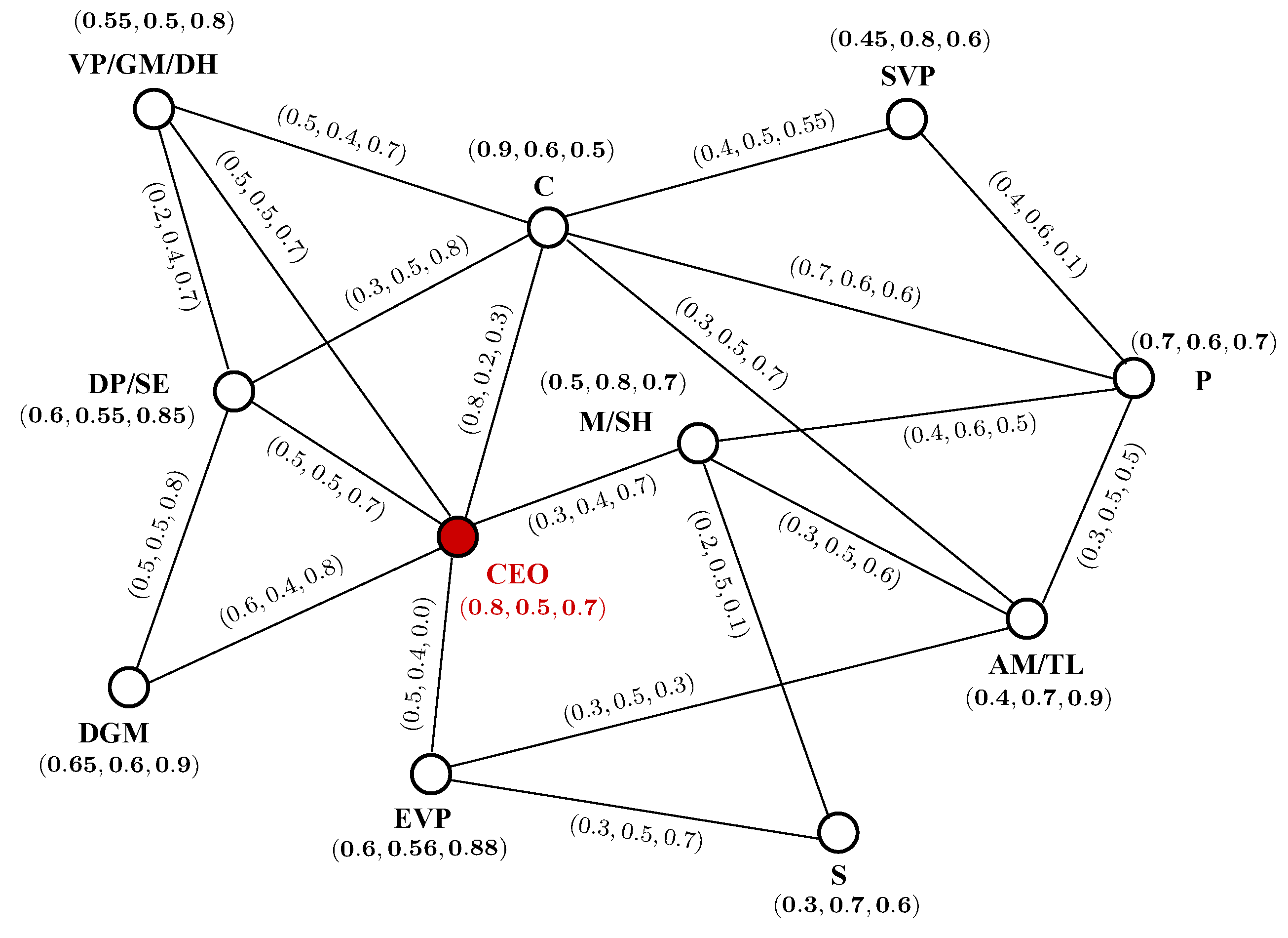
Figure 29 displays a 4-RPFG representing the social network composed of 11 different employees.

There are 11 different q-RPF ego networks/graphs associated with the given q-RPF network/graph, where the vertices/nodes represent the powers of employees in the company, and edges/links represent their relationships. The membership functions ${\mu }_{\mathcal{P}},{\eta }_{\mathcal{P}},$ and ${\nu }_{\mathcal{P}}$ in triplet $({\mu }_{\mathcal{P}},{\eta }_{\mathcal{P}},{\nu }_{\mathcal{P}})$, assigned to each node, indicate their positive impact, their neutral behavior, and their negative impact within the company, respectively. For example, $(0.8,0.5,0.7)$ tells the status level of the CEO as: the CEO possesses $40.96\%$ positive impact, and $24.01\%$ negative impact within the company. A total of $6.25\%$ of his behavior is neutral. While the refusal degree $\pi =\sqrt[4]{1-{0.8}^4-{0.5}^4-{0.7}^4}$ of CEO indicates that only $28.78000001\%$, he has the ability to refuse to participate in the company’s matters. However, the positive, neutral, and negative membership degrees ${\mu }_{\mathcal{Q}},{\eta }_{\mathcal{Q}},$ and ${\nu }_{\mathcal{Q}}$ of edges depict the positive associations, abstinence to associate, and negative associations among employees. For example, the edge between president and assistant manager is assigned by triplet $(0.3,0.5,0.3).$ The relationships between them can be translated by a means of q-rung picture fuzzy analysis as follows: they have only $0.81\%$ positive attitude. The neutral and negative behavior have same the weight, i.e., $6.25\%$ and $86.69\%$ of interactions translate the extent of the clash between them. Similar considerations can be extracted from other edges. The corresponding adjacency matrix is shown in

Table 2. Adjacency matrix corresponding to Figure 29.

	C	CEO	P	DP/SE	EVP	SVP	VP/GM/DH	DGM	M/SH	AM/TL	S
C	$(0.0,0.0,0.0)$	$(0.8,0.2,0.3)$	$(0.7,0.6,0.6)$	$(0.3,0.5,0.8)$	$(0.0,0.0,0.0)$	$(0.4,0.5,0.55)$	$(0.5,0.4,0.7)$	$(0.0,0.0,0.0)$	$(0.0,0.0,0.0)$	$(0.3,0.5,0.7)$	$(0.0,0.0,0.0)$
CEO	$(0.8,0.2,0.3)$	$(0.0,0.0,0.0)$	$(0.0,0.0,0.0)$	$(0.5,0.5,0.7)$	$(0.5,0.4,0.0)$	$(0.0,0.0,0.0)$	$(0.5,0.5,0.7)$	$(0.6,0.4,0.8)$	$(0.3,0.4,0.7)$	$(0.0,0.0,0.0)$	$(0.0,0.0,0.0)$
P	$(0.7,0.6,0.6)$	$(0.0,0.0,0.0)$	$(0.0,0.0,0.0)$	$(0.0,0.0,0.0)$	$(0.0,0.0,0.0)$	$(0.4,0.6,0.1)$	$(0.0,0.0,0.0)$	$(0.0,0.0,0.0)$	$(0.4,0.6,0.5)$	$(0.3,0.5,0.5)$	$(0.0,0.0,0.0)$
DP/SE	$(0.3,0.5,0.8)$	$(0.5,0.5,0.7)$	$(0.0,0.0,0.0)$	$(0.0,0.0,0.0)$	$(0.0,0.0,0.0)$	$(0.0,0.0,0.0)$	$(0.2,0.4,0.7)$	$(0.5,0.5,0.8)$	$(0.0,0.0,0.0)$	$(0.0,0.0,0.0)$	$(0.0,0.0,0.0)$
EVP	$(0.0,0.0,0.0)$	$(0.5,0.4,0.0)$	$(0.0,0.0,0.0)$	$(0.0,0.0,0.0)$	$(0.0,0.0,0.0)$	$(0.0,0.0,0.0)$	$(0.0,0.0,0.0)$	$(0.0,0.0,0.0)$	$(0.0,0.0,0.0)$	$(0.3,0.5,0.3)$	$(0.3,0.5,0.7)$
SVP	$(0.4,0.5,0.55)$	$(0.0,0.0,0.0)$	$(0.4,0.6,0.1)$	$(0.0,0.0,0.0)$	$(0.0,0.0,0.0)$	$(0.0,0.0,0.0)$	$(0.0,0.0,0.0)$	$(0.0,0.0,0.0)$	$(0.0,0.0,0.0)$	$(0.0,0.0,0.0)$	$(0.0,0.0,0.0)$
VP/GM/DH	$(0.5,0.4,0.7)$	$(0.5,0.5,0.7)$	$(0.0,0.0,0.0)$	$(0.2,0.4,0.7)$	$(0.0,0.0,0.0)$	$(0.0,0.0,0.0)$	$(0.0,0.0,0.0)$	$(0.0,0.0,0.0)$	$(0.0,0.0,0.0)$	$(0.0,0.0,0.0)$	$(0.0,0.0,0.0)$
DGM	$(0.0,0.0,0.0)$	$(0.6,0.4,0.8)$	$(0.0,0.0,0.0)$	$(0.5,0.5,0.8)$	$(0.0,0.0,0.0)$	$(0.0,0.0,0.0)$	$(0.0,0.0,0.0)$	$(0.0,0.0,0.0)$	$(0.0,0.0,0.0)$	$(0.0,0.0,0.0)$	$(0.0,0.0,0.0)$
M/SH	$(0.0,0.0,0.0)$	$(0.3,0.4,0.7)$	$(0.4,0.6,0.5)$	$(0.0,0.0,0.0)$	$(0.0,0.0,0.0)$	$(0.0,0.0,0.0)$	$(0.0,0.0,0.0)$	$(0.0,0.0,0.0)$	$(0.0,0.0,0.0)$	$(0.3,0.5,0.6)$	$(0.2,0.5,0.1)$
AM/TL	$(0.3,0.5,0.7)$	$(0.0,0.0,0.0)$	$(0.3,0.5,0.5)$	$(0.0,0.0,0.0)$	$(0.3,0.5,0.3)$	$(0.0,0.0,0.0)$	$(0.0,0.0,0.0)$	$(0.0,0.0,0.0)$	$(0.3,0.5,0.6)$	$(0.0,0.0,0.0)$	$(0.0,0.0,0.0)$
S	$(0.0,0.0,0.0)$	$(0.0,0.0,0.0)$	$(0.0,0.0,0.0)$	$(0.0,0.0,0.0)$	$(0.3,0.5,0.7)$	$(0.0,0.0,0.0)$	$(0.0,0.0,0.0)$	$(0.0,0.0,0.0)$	$(0.2,0.5,0.1)$	$(0.0,0.0,0.0)$	$(0.0,0.0,0.0)$

, where the degrees for each edge $uv$ in $\mathcal{G}=(\mathcal{P},\mathcal{Q})$ are evaluated using the following relations:

$$\begin{array}{ccc}\hfill {\mu }_{\mathcal{Q}}(uv)& \le & {\mu }_{\mathcal{P}}(u)\wedge {\mu }_{\mathcal{P}}(v),\hfill \\ \hfill {\eta }_{\mathcal{Q}}(uv)& \le & {\eta }_{\mathcal{P}}(u)\wedge {\eta }_{\mathcal{P}}(v),\hfill \\ \hfill {\nu }_{\mathcal{Q}}(uv)& \le & {\nu }_{\mathcal{P}}(u)\vee {\nu }_{\mathcal{P}}(v).\hfill \end{array}$$

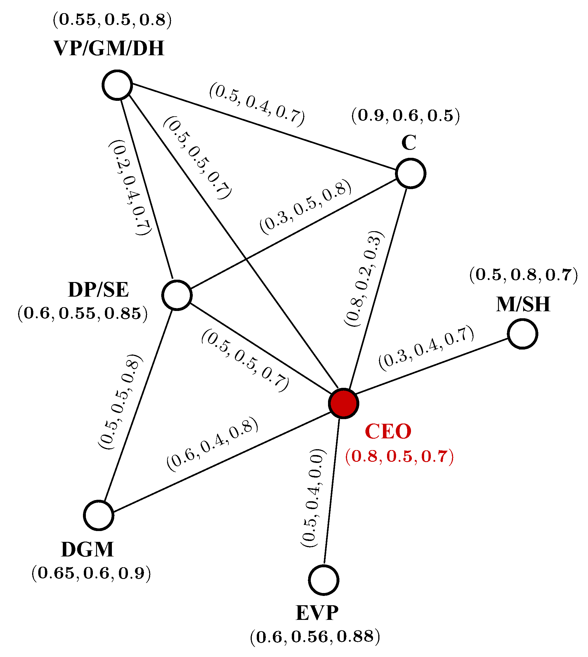
The CEO is a company’s top decision-maker, and all other executives answer to him/her. Next, we want to study the powers of the CEO in this company, and his associations with other executives. For this, we consider the CEO as ego, and extract a q-rung picture fuzzy ego network from a q-rung picture fuzzy social network (see Figure 29) according to Algorithm 1.

Figure 30 displays a q-rung picture fuzzy ego network $\mathcal{H}=(\mathcal{A},\mathcal{B})$ for selected ego, i.e., CEO (colored node).

The CEO influences the executives who are board members, and jointly supervise the activities of company. The titles designate an individual as an officer of the company with specific responsibilities that make them legally accountable in their position. The following investigations provide a q-RPF social network analysis for the CEO:

• The impact of CEO is equally distributed with the vice president, and deputy president as the positive, neutral, and negative associations of both are $6.25\%,6.25\%,$ and $24.01\%,$ respectively.
• The CEO greatly refuses to value the inputs of executive vice present for strategic initiatives as there is $91.19\%$ refusal part while no negative associations between them, where the positive associations are $6.25\%,$ and $2.56\%$ is the neutrality in their behavior.
• By means of the positive and negative associations of the CEO with the Chairman, the founder of the company, we can this interpret as: the Chairman works $40.96\%$ on the CEO’s opinion, for $0.81\%$, he works opposite of his opinion, for $0.16\%$, his behavior is neutral with the CEO, and, for $58.07\%$, the chairman refuses to trust his part.
• The reporting relationships between general manager, and CEO is $12.96\%$ positive, $2.56\%$ neutral, and $40.96\%$ negative, while, for $56.48\%$ of his own part, the general manager refuses to report to him.
• Between the vice president and deputy president, there is less positive $(0.16\%),$ and high negative $(24.01\%)$ associations, which indicate their history of conflict.
• The manager being a section head has to resolve all cases in his section to answer to the CEO. The absence of edge with the executive vice president show that he has no concern with the executive vice president in company’s matters.

The similar investigations can be seen between executives (alters) in the q-RPF ego-network (Figure 30).

5. Conclusions

Real life situations are often very uncertain and vague in nature. Due to a lack of information, the future state of system might not be completely known. The notion of fuzzy set offers a suitable departure point for the creation of such a framework which has potentially wider scope of applicability. The picture and spherical fuzzy models are a good way to tackle the uncertain information, when people think about not only the reaction is positive or negative, but there are some abstinence and refusal. The q-RPF model is more efficient than picture and spherical fuzzy models because it provides a wide space of permissible triplets. In the present study, we have explored some graph-theoretic ideas under q-RPF circumstances. Regularity is one of the attributes that permits many of the challenges connected with graph analysis to be addressed. The present study has provided a novel description on edge regularity of q-RPFGs and developed several related results. In particular, the edge regularity of square q-RPFGs and q-RPF line graphs has been illustrated. These graphs have eventually helped to link certain q-RPF systems and crisp systems allowing for greater ease in computing properties of these q-RPF systems for modeling purposes or optimizing q-RPF networks. Moreover, the q-RPFLGs can be applied to work out extremal problems. We have also established the relationships between regular and edge regular q-RPFGs. Finally, we have presented the concept of q-RPF ego-networks to extract knowledge from large social networks as an application. Our future work will expand on these terms: (1) Interval-valued q-RPFGs; (2) Bipolar-valued q-RPFGs; and (3) Hesitant q-RPFGs.