End-to-End Mandarin Speech Recognition Combining CNN and BLSTM

Abstract

Since conventional Automatic Speech Recognition (ASR) systems often contain many modules and use varieties of expertise, it is hard to build and train such models. Recent research show that end-to-end ASRs can significantly simplify the speech recognition pipelines and achieve competitive performance with conventional systems. However, most end-to-end ASR systems are neither reproducible nor comparable because they use specific language models and in-house training databases which are not freely available. This is especially common for Mandarin speech recognition. In this paper, we propose a CNN+BLSTM+CTC end-to-end Mandarin ASR. This CNN+BLSTM+CTC ASR uses Convolutional Neural Net (CNN) to learn local speech features, uses Bidirectional Long-Short Time Memory (BLSTM) to learn history and future contextual information, and uses Connectionist Temporal Classification (CTC) for decoding. Our model is completely trained on the by-far-largest open-source Mandarin speech corpus AISHELL-1, using neither any in-house databases nor external language models. Experiments show that our CNN+BLSTM+CTC model achieves a WER of 19.2%, outperforming the exiting best work. Because all the data corpora we used are freely available, our model is reproducible and comparable, providing a new baseline for further Mandarin ASR research.

1. Introduction

With the rapid development of smart devices such as mobile phones and robots, users increasingly interact with man–machine interfaces via speech recognition. Google Now, Apple Siri, and Microsoft Cortana are all widely used systems that rely on Automatic Speech Recognition (ASR). Besides, Baidu IME and iFLY IME can map Mandarin and English utterances to corresponding texts. Furthermore, recently in January 2019, Alibaba Cloud Computing published its Distributed Speech Solution. By combining ASR technique with devices such as switch panel or air conditioner, it helps to easily deploy speech recognition systems indoors. More than that, speech recognition can also offer lots of help in other domains such as auto driving, health care, etc.

Decades of hand-engineered domain knowledge has gone into current state-of-the-art ASR pipelines. Conventionally, Large Vocabulary Continuous Speech Recognition (LVCSR) systems often contain several separate modules, including acoustic, phonetic, language models, and some special lexicons. All these modules in an ASR system are trained separately. As a result, errors of every module would extend during the recognizing process. More than that, building an ASR with so many modules requires varieties of hand-engineered domain knowledge such as pronunciation lexicon, linguistic expertise, etc. All these make it hard to design and train a good-performing ASR system.

Since conventional ASR has many disadvantages, recently a powerful alternative solution is proposed to train ASR models end-to-end, replacing most modules with a single deep learning model [1,2]. The ‘end-to-end’ vision of training can substantially simplify the training process by removing the engineering required for the bootstrapping/alignment/clustering/HMM machinery often used to build state-of-the-art ASR models. On a system built on end-to-end deep learning, We can employ a range of the newest deep learning techniques to train a novel deep neural model with high performance.

Enough data is the key for end-to-end ASRs to achieve better performance than conventional ASRs. For English ASR, large-amount databases such as TED-LIUM [3] and Librispeech [4] offer open platforms for both researchers and industrial developers to experiment and compare system performances. Thanks to the popularization of smart devices, it becomes much easier than before for industries to access and collect large amount of speech data for Mandarin ASR. However, as most of these data are not shared with the public, researchers still have very limited access to large-amount real-world Mandarin speech data. As a result, Mandarin ASR research works do not scale well to industrial scenarios. Besides, since existing state-of-the-art Mandarin ASR works all use in-house large-amount dataset, comparing with them is pointless and sheds little light on future research.

Fortunately, a freely-available Mandarin speech corpus, AISHELL-1 [5], is released recently. It is by far the largest free-accessed Mandarin corpus, containing 400 speakers and over 170 h of Mandarin speech data. It is suitable for conducting and comparing speech recognition research works for Mandarin.

In this paper, we propose an end-to-end Mandarin ASR model that combines Convolutional Neural Net (CNN) and Bidirectional Long-Short Time Memory (BLSTM) Neural Net, named CNN+BLSTM+CTC. This model uses CNN to learn local features in frequency and time domain, uses BLSTM to learn history and future contextual features. Our model is reproducible and comparable for other researchers because it is trained on the open-accessed Mandarin Speech Dataset AISHELL-1, using neither other in-house data nor external language model. We benchmark our CNN+BLSTM+CTC on AISHELL-1 test dataset and compare it to some existing works, Experiments results show that our model gets a WER of 19.2%, outperforming existing methods in [6,7].

The contribution of this paper is three-fold:

• We propose CNN+BLSTM+CTC, an end-to-end ASR model using both CNN and BLSTM. It combines CNN layer’s ability of learning local features and BLSTM layer’s ability of learning history and future contextual features, enabling the CNN+BLSTM+CTC to model audio signals effectively and make precise recognition.
• We use neither in-house training data no external language model in this paper. All the training, development, testing data we used come from dataset AISHELL-1, which can be freely acquired. This makes our results comparable for other researchers.
• We carry out comprehensive experiments to verify our design ideas. Experiments results show that our CNN+BLSTM+CTC makes effective speech recognition.

The remainder of the paper is organized as follows. We begin with a review and analysis of related works in conventional ASR, end-to-end ASR, especially Mandarin end-to-end ASR in Section 2. Section 3 describes the architecture and detail design of our CNN+BLSTM+CTC model. We describe experiment settings, analyze the results for our model and compare it with existing works in Section 4. We conclude our work in Section 5 and list some future works in Section 6.

2. Related Works

Commonly, for an input utterance, conventional state-of-art ASR systems use HMM-based acoustic model to extract acoustic features, use GMM-based pronunciation model to map acoustic features to sub-phonetic states and use pronunciation lexicon to map sub-phonetic states to a sequence of words. Finally, the word sequence is rescored by external language model to generate a reasonable sentence. Models working in such way have many disadvantages.

• Building such an ASR system is a very tough work. Firstly, there are many modules in such a system such as acoustic model, language model, to name but a few. Secondly, different domain knowledge and expert engineering work are needed to design these different modules. For example, a linguistics expert may be needed to design the language model.
• Training a good-performing model is very hard. Since different modules are designed based on different hypotheses, they need different expertise for training. What makes things worse, each of them has its own optimizing objectives, which may be different from each other and even different from the global optimizing objective. All these together make it difficult to train a good-performing model.
• These models are awkward to fine tune. As they contain many modules, when we want to adapt them to recognize speeches in a new scenario, most of these modules must be retrained from scratch, which will cost a lot of time and effort.
• Structure of such models is inflexible. Modules contained in a conventional model and the structure between these modules are almost fixed. It is hard to add/delete/change a module or reorganize their structure. Thus, it is difficult to introduce new developed technologies such as deep learning into these models.
• These models need high-quality dataset for training. The training data must be aligned, which means that every input frame must have a corresponding label. Building such a dataset takes masses of time, effort and domain knowledge, and must be very careful. As a result, it is almost impossible to build a large-scale dataset.

Recently, researchers have been working on end-to-end ASR methods to overcome these disadvantages of conventional ASR.

End-to-end ASR is a kind of sequence-to-sequence model. In contrast to conventional ASR that contains many modules and derives the final result from several intermediate states, end-to-end ASR directly maps input acoustic signals to graphemes such as characters or words. It subsumes most modules into a DNN and use an overall training objective function to optimizes the criteria that related to the final evaluation criterion we really concern about (in most cases, it is the Word Error Rate, WER). However, in conventional ASR, every module has its own objective function, which is indirectly related to the final evaluation criterion.

By mapping input sequence directly into output sequence, end-to-end ASR can effectively simplify the ASR pipelines.

However, training a state-of-the-art end-to-end ASR requires very large amount of labeled training data. However, existing labeled and aligned datasets are too small in scale. Besides, these existing datasets are labeled at frame level. To get the final text sequence, researchers must design some modules to map frame-level label sequence to text sequence. As a result, end-to-end ASR cannot develop rapidly unless unaligned speech datasets can be used for training.

Connectionist Temporal Classification (CTC) technique makes it come true.

In 2006, Graves [8] proposed CTC. CTC solves two main problems for end-to-end ASR. Firstly, there is no need to segment and align the speech data any more. CTC introduces a blank label ‘-’ which means ’no output at this moment’. Based on the blank label, it designs the intermediate structure of path. By removing all repeated and blank labels in paths, some of the paths can be subsumed into a final label sequence. Therefore, without segmentation and alignment, CTC can still map input sequence to output sequence. Secondly, there is no need to design external modules to post-process the output sequence of CTC, now that CTC’s output sequence is exactly what we expected (e.g., a reasonable sentence).

After the proposal of CTC, end-to-end ASR develops rapidly.

Graves [2] presents a system using bidirectional RNN and CTC to recognize speech at character-level. The system uses 5 bidirectional RNN layer and 1 CTC layer to get character sequence from input acoustic spectrogram. It also uses an external language model and a new loss function called Expected Transcription Loss to improve the performance. Combining all these together, the system is competitive to the state-of-the-art method on Wall Street Journal corpus. While using this system to rescore a DNN-HMM-based model, it achieves new state-of-the-art performance, with WER of 6.7%.

Based on [2], there are many refinements proposed. Hannun [9] finds that the best performance in [2] still relies on HMM infrastructure. They present a method which only use neural network and language model for speech recognition, discarding the HMM infrastructure. This method uses 5 neural layers, the third of which is bidirectional RNN. It uses CTC during training, while for decoding it uses a new-designed prefix beam search algorithm that incorporate a language model. This decoding algorithm equips speech recognition system with first-pass decoding. Although the system’s performance on Wall Street Journal Corpus does not outperform the best HMM-based method, it demonstrates the promise of CTC-based end-to-end ASR. Experiments also show that method using RNN outperforms that using DNN substantially, and bidirectional RNN outperforms RNN. Besides, they find that model’s structure is more influential than its total number of free parameters.

The work in [10] is another refinement of [2], its purpose is redesigning the rescore algorithm and enabling first-pass decoding, too. It uses a model with the same structure as in [9], but they use different decoding algorithms and language models. In [9], the decoding is word-level, the language model is n-gram model. while in [10], the decoding is character-level, the language model is a neural type. Besides, Experiments in [10] are carried out on the SwitchBoard conversational telephone speech corpus dataset, not on the WSJ dataset. Its final performance is comparable to the HMM-GMM baseline in Kaldi.

Sak [11] presents a bidirectional LSTM+CTC model, and uses many tricks to improve its performance. It stacks input frame and uses sub-sampling with $stride=2$, aiming to represent long-term features and reduce computation. The output of CTC is Context-Dependent phonetic units, rather than phonemes used in other works. After being trained by CTC, the model also uses state-level minimum Bayes risk (sMBR) sequence discriminative training criterion to improve its performance. Finally, it outperforms conventional sequence trained LSTM-hybrid models.

Although having made great improvement, most of the end-to-end ASR mentioned above only output character-level labels or phones. They need an external lexicon to map phones or characters to words, or sentences. Some researchers think they are not ’real’ end-to-end ASRs.

Soltau [12] presents an LVCSR system with whole words as acoustic units. The system uses deep bidirectional LSTM RNNs and CTC to output words directly. It contains 7 bidirectional LSTM, using no language model. Training data contains 125,000 h of speech data from YouTube, with a vocabulary of about 100,000 words. Experiments show that this system performs better than CD-phone-based model. It also shows that language model has relatively small impact on this system’s accuracy. Thus, we can see that if the training transcriptions set is large enough, a neural network model can learn linguistic knowledge implicitly and achieve comparable accuracy, without need for an external language model.

Audhkhasi [13] uses SwitchBoard dataset to develop end-to-end ASR system. It also maps utterance directly to words. This work designs a model with 5 bidirectional LSTM and a full connected layer. It uses weights from a pre-trained phone-CTC model to initialize the bidirectional LSTM and uses a pre-trained word-embedding matrix to initialize the full connected layer. On the Swithcboard/CallHome test set it achieves WER of 13.0%/18.8% (using no language model) and 12.5%/18.0% (using a language model).

Having done a lot of work to develop end-to-end ASRs, researchers conclude that large-scale data and large model are very crucial to improve performance. There are many works on data augmentation and large-scale GPU training.

Hannun [1] presented DeepSpeech system in 2014. It is an English speech recognition system using CNN, bidirectional RNN, CTC, and language model. The key in DeepSpeech is a well-optimized RNN training system using multiple GPUs (enabling data and model parallelism), and a novel data augmentation method (including tricks such as Synthesis by superposition, Capturing Lombard Effect, left and right translation) to obtain large amounts of training data. This makes it possible to train the DeepSpeech on thousands of hours of speech data. With enough training data, the DeepSpeech model can be trained robust to noise and speakers. It uses CTC loss function for training and language model for decoding. Experiments on SwitchBoard show that for clean conversation speech recognition, DeepSpeech achieves WER of 16%, which is the state-of-the-art performance. Other experiments on a constructed noisy speech data show that DeepSpeech outperforms systems from business companies include Apple, Google, Bing, and wit.ai, achieving the best performance.

In 2016, Amodei presented DeepSpeech2 [14], which outperforms human workers in some speech recognition tasks. DeepSpeech2 is an RNN+CTC model, with one or more CNN layer, several RNN(bidirectional or unidirectional) layer. CTC loss function is used for training. However, an algorithm incorporating CTC, language model, and label sequence length is used for decoding. Although it uses many training tricks such as batch normalization, SortaGrad, frequency convolution, and lookahead convolution, the key to DeepSpeech2 is its HPC technologies. It creates customized All-Reduce code for OpenMPI to sum gradients across GPUs on multiple node, develops a fast implementation of CTC for GPUs, and use custom memory allocators. Taken together, these techniques enable DeepSpeech2 to sustain overall 45% of theoretical peak performance on each node, which allows it to iterate more quickly to identify superior architectures and algorithms. Experiments on Wall Street Journal corpus, LibriSpeech, and an in-house Mandarin corpus show that for formal clean English and Mandarin speech recognition, DeepSpeech2 can outperform human workers. However, as to accented or noisy speech recognition, human workers still achieve better WERs.

However, most of the works mentioned above are presented on English speech data. There are relatively few works on Mandarin data. while some large-amount datasets are freely accessed for English ASR, end-to-end Mandarin ASR research is hindered by lack of large-amount data.

For Mandarin ASR, the most popular dataset is RAS-863 database [15]. It involves continuous reading speech of more than 80 speakers, in total about 100 h speech data. However, this database is not open-accessed. Besides RAS-863, there are also some other commercial datasets that can be purchased from DataTang (www.datatang.com) and Speech Oceanf (www.speechocean.com). However, there are only a few open-accessed Mandarin datasets of very small amount:

• THCHS-30 [16]: The name ‘THCHS-30’ stands for ‘Tsinghua Chinese 30-hour database’. This database is connected by Dong Wang in 2001 and is opened to the public in 2015. It involves 35 h reading speech data produced by 50 speakers. The speech signals are recorded in silent office and released along with lexicon, language model, and training recipe. It also provides three kinds of noise: white, car, and cafeteria noise. This database is the first release that can be used to build a practical Mandarin speech recognition system.
• OC16-CE180 [17]: The OC16-CE80 Chinese-English mix-lingual speech database was released as a main resource for training, development and test for the Chinese-English mix-lingual speech recognition (MixASR-CHEN) challenge on O-COCOSDA 2016. This database consists of 80 h speech signals recorded from more than 1400 speakers. The utterances are in Chinese, but each involves one or several English words.
• AISHELL-1 [5]: Beijing ShellShell Company (www.aishelltech.com) releases the AISHELL-1 corpus which is by far the largest open-source Mandarin ASR corpus. This corpus covers 5 domains including ‘Finance’, ‘Science and Technology’, ‘Sports’, ‘Entertainments’ and ‘News’. It consists of over 170 h of Mandarin speech data recorded from 400 speakers coming from different accent areas in China. The corpus is released along with a GMM-HMM Kaldi recipe, which are publicly available and free for academic research.

As is by far the largest open-accessed corpus, there are some end-to-end Mandarin ASR presented on AISHELL-1 after the dataset was released.

Some of these works are not LVCSR but other speech tasks. For example, Chen [18] uses AISHELL-1 as a sub-task in multi-task model to help recognizing under-resourced languages such as Vietnamese and Singapore Hokkien. Zhou [19] uses it for speaker embedding. Tu [20] uses it for automatic pronunciation evaluation. Zhang [21] uses it as test data to evaluate language model. Lugosch [22] uses it to recognize tones in continuous speech for tonal languages.

However, despite these works, the AISHELL-1 is mostly used for Mandarin ASR.

Wang [6] presents a CNN+BLSTM+CTC structured end-to-end ASR. The system involves 2 CNN layers, 1 max pooling layer, 2 bidirectional LSTM layers, and a full connected layer. It uses convolution and sub-sampling in both time and frequency domain. It also uses Limited Weight Sharing instead of Full Weight Sharing. Experiments on AISHELL-1 show that without external language model, the CNN+BLSTM+CTC system achieves WER of 20.68%, while using an external language model, the WER drops to 14.16%.

This is a helpful work because all the database it used is Mandarin corpus AISHELL-1 (only consider the model without language model). Therefore, it is possible for other researchers to reproduce its work and meaningful to compare with it, which is important to conduct new research works.

Li [7] proposes an encoder-decoder structured end-to-end Mandarin ASR involving Adaptive Computation Steps (ACS) algorithm, which enables the ASR to determine how many speech frames should be considered before outputting a new label. The encoder is a pyramidal RNN net which sub-samples current layer’s hidden state before transmitting it to the next layer. This sub-sampling reduces computing steps and speeds up computation. The decoder contains a halting layer and a decoding layer. At every step, the halting layer uses the sum of some early steps’ probabilities to determine whether it should output a label, while the decoding layer determines which label it should output. Thus, at every time step, the system only concerns about a continuous speech block related to the output label, rather than all the speech sequence. With an RNN language model, this model achieves WER of 18.7% on the AISHELL-1 corpus.

Li [23] thinks it is helpful to use future contextual information in acoustic model. However, building a model that uses future contextual information while keeping a low latency at the same time is difficult. Li [23] presents a system trying to overcome this difficulty. Firstly, the system designs the mGRUIP which is a mGRU with an additional inside projection layer. This projection layer compresses the inputs and hidden states to reduce the number of parameters and computation. Secondly, it designs temporal encoding and temporal convolution to encode future contextual information. All these together enables the model to use future contextual information while keeping a low latency. Trained on a 1400 h in-house speech data, the model achieves CER of 5.71% on AISHELL-1 test set. However, experiments on SwitchBoard show that the system’s latency on English recognition is 170 ms.

Li’s work in [24] is a revision of work in [23]. It improves the mGRUIP structure for higher performance. Firstly, for update gate and activation in the RNN cell, it adds batch normalization on both ItoH (input to Hidden) and HtoH (Hidden to Hidden) connection. Secondly, it enlarges the context scope to capture not only future but also history contextual information. Experiments show that trained on a 1600 h in-house speech data, the system achieves about 4% CER on AISHELL-1 test set. However, trained on a 10,000 h in-house speech data, the CER drops to 3.55%.

As we can see, works in [23,24] achieved impressive good performance. However, since they both use large-amount dataset which is not open-accessed, they help little for researchers who have no access to those datasets, and therefore shed little light on what a good model should be like. In this paper, we use the AISHELL-1 corpus to train an end-to-end Mandarin ASR. Without any external in-house training data or special language model, our system achieves state-of-the-art performance. Not only that, but our results are meaningful to compare with for other research works, providing a new baseline.

3. End-to-End Model for Mandarin ASR

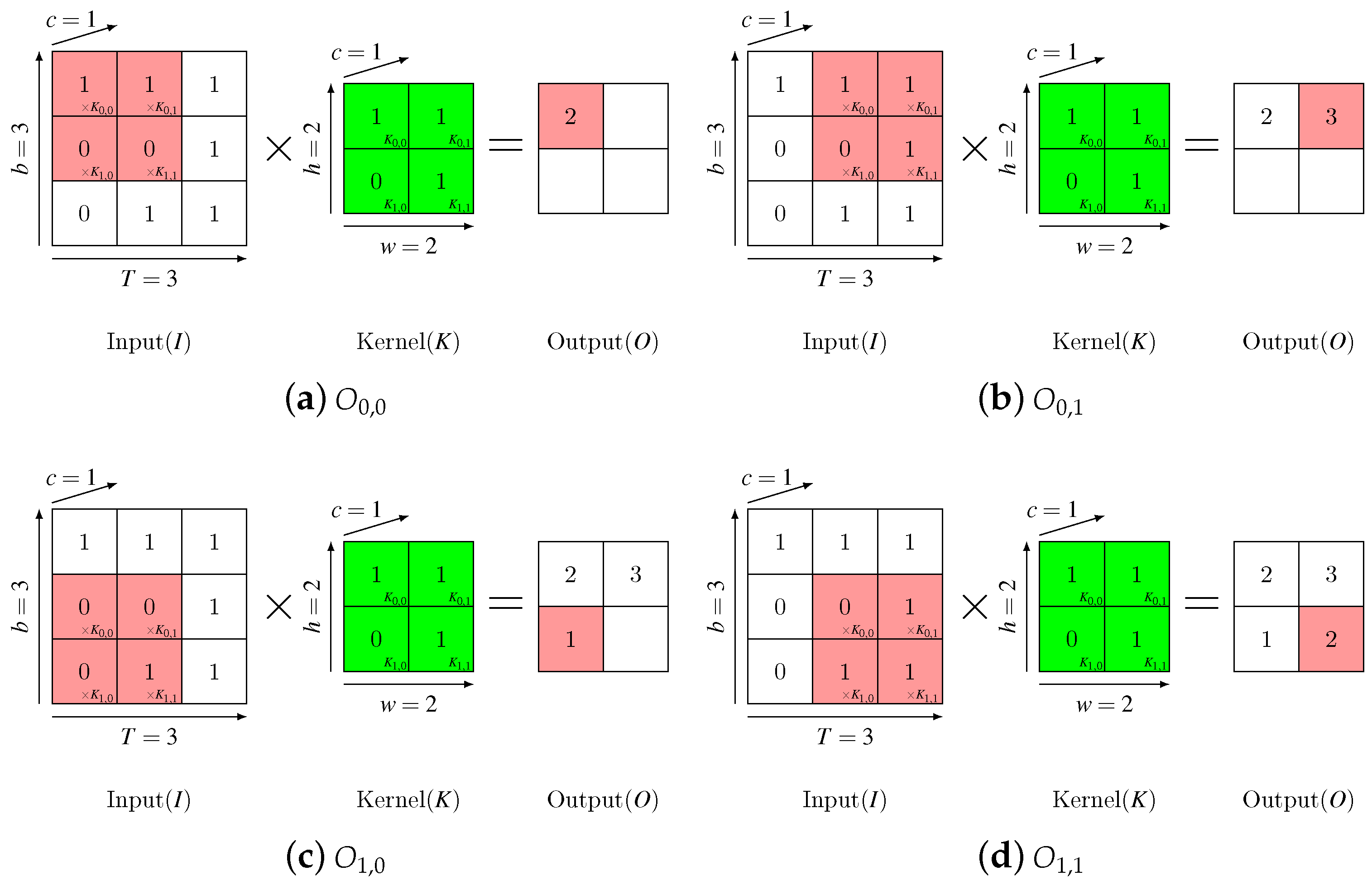
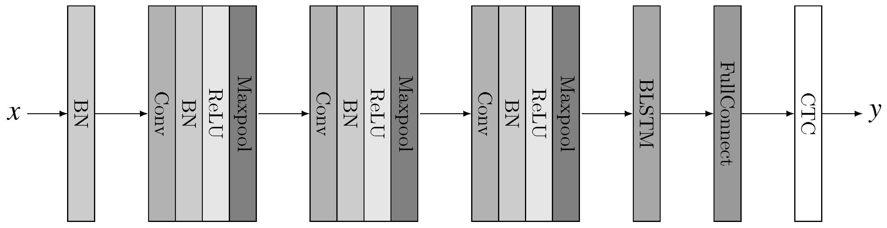
Figure 1 illustrates the architecture of our deep neural network. The audio input x is firstly batch normalized, then passed through 3 CNN blocks, each of which involves 4 operations: Convolution, Batch Normalization, Rectified Linear Unit (ReLU) activation and max pooling. The CNN blocks are followed by a bidirectional LSTM layer and a full connected layer. At last a CTC layer does the decoding and outputs the label sequence y.

In the following part of this section we will describe our design ideas in detail.

3.1. Convolution Layer

Given a input sequence $X=\{x_1,\cdots ,x_T\},x_i\in R^{b\times c}$, a 1-filter convolution kernel $K\in R^{w\times h\times c}$ with convolution strides $SC=(s{w}_c,s{h}_c)$. The convolution result is a 2-dimensional feature map, which is calculated as in Equation (1):

$$o_{i,j}=\sum _{w_i,h_j,q}{x}_{s{w}_c·i+w_i,s{h}_c·j+h_j,q}·k_{w_i,h_j,q}$$

(1)

where T, c, b are the time steps, channels and bandwidth of input sequence respectively, w, h are the kernel’s width and height respectively, $s{w}_c$, $s{h}_c$ are the width and height stride of convolution respectively.

If the kernel has more than 1 filters, the convolution will get more than 1 feature maps.

Works in different papers use different features as the input sequence $\{x_1,\cdots ,x_T\}$. While most works use cepstral coefficients, there are some works using the raw waveform. In this paper, the inputs $\{x_1,\cdots ,x_T\}$ are Mel-Frequency Cepstral Coefficients. The convolution kernel K is a matrix. It works on local patches of inputs and slides along T-dimension and b-dimension.

Figure 2 illuminates a simple procedure of CNN with only one filter, where $T=3$, $b=3$, $c=1$, $w=2$, $h=2$, $s{w}_c=1$, $s{h}_c=1$.

From Equation (1) we can see that every result element $o_{i,j}$ of convolution is derived from $w\times h$ local elements in every input feature map. Thus, for convolution on an input sequence with c feature maps, every result element is correlated with $w\times h\times c$ local input elements. This means that the convolution can capture input data’s local features at corresponding position.

Convolution’s ability of learning local features suits speech recognition task very well. ASR never gives output depending only on a single momentary input signal. In fact, no matter to utter or recognize a piece of speech, the speech is always treated as a sequence of short audio segments which last for hundreds of microseconds. Therefore, learning the local features on short acoustic segments is a significant step for speech recognition.

One CNN layer can only cover a small input scope, but if we stack many CNN layers together, they can learn the local features of a much larger scope.

To simply the analysis, let us only consider the time axis. Assume the CNN kernel’s width is $w_c$, width stride is $s{w}_c$. We refer to the time span covered by result element as $t_c$, and refer to the time shift window between two adjacent result element as $windo{w}_c$. Then, $t_c$ and $windo{w}_c$ can be calculated according to the following Equation (2):

$$\begin{array}{cc}\hfill t_c& =t_i+(w_c-1)·windo{w}_i\hfill \\ \hfill windo{w}_c& =s{w}_c·windo{w}_i\hfill \end{array}$$

(2)

where $t_i$ and $windo{w}_i$ are the time scope and shift window of input.

In this paper, we use Mel-Frequency Cepstrum Coefficient (MFCC) sequence as the input. Every MFCC frame’s time span is 25 ms and the shift window is 10 ms. 3 CNN layers’ kernel width on the time dimension are respectively 3, 2, and 2. Their convolution strides are all 1. Therefore, without pooling layer, result element of the last CNN layer covers a time span of 65 ms, and its shift window between two adjacent element is 10 ms, which means that the 3-layer CNN can learn local features of every 65 ms, much larger than the original MFCC frame’s time span.

3.2. Batch Normalization

Training Deep Neural Networks is complicated by the fact that the distribution of each layer’s inputs changes during training, as the parameters of the previous layers change. Since the inputs to each layer are affected by the parameters of all preceding layers, small changes to the network parameters amplify as the network becomes deeper. The change in the distribution of network activations due to the change in network parameters during training is defined as Internal Covariate Shift. Batch normalization is designed to alleviate this Internal Covariate Shift by introducing a normalization step that fixes the means and variances of layer inputs.

Batch Normalization (BN) [25] is widely used in deep learning and brings remarkable improvement in many tasks. It allows researchers to use much higher learning rates and be less careful about initialization. It helps to accelerate training speed and improve the performance substantially. In this work, we use BN between convolution and activation.

Formally, for a batch $X=\{x_1,\cdots ,x_m\}$ of size m, where every $x_i$ is a d-dimension vector, $x_i=\{x_i^1,\cdots ,x_i^d\}$, BN of every $x_i$ is

$$bn\left(x_i\right)=\{bn\left(x_i^1\right),\cdots ,bn\left(x_i^d\right)\}$$

(3)

where $bn\left(x_i^k\right)$ is

$$bn\left(x_i^k\right)=\frac{x_i^k-E\left[x^k\right]}{\sqrt{Var\left[x^k\right]}}$$

(4)

and

$$E\left[x^k\right]=\frac{1}{m}\sum _{i=1}^m{x}_i^k$$

(5)

$$Var\left[x^k\right]=\frac{1}{m}\sum _{i=1}^m{(x_i^k-E\left[x^k\right])}^2$$

(6)

Please note that simply normalizing each input of a layer may change what the layer can represent. To accomplish this, a pair of parameters ${\gamma }^k$ and ${\beta }^k$ are introduced for each dimension k, and the final BN result is $bn\left(x_i\right)=\{y_i^1,\cdots ,y_i^d\}$ where $y_i^k={\gamma }^{k}bn\left(x_i^k\right)+{\beta }^k$.

During training, the batch size m is larger than 1. However, during inferring, $m=1$. Therefore, we cannot calculate the means and variances of the layer inputs. So, the means and variances calculated during training are used for inferring.

However, BN is neither necessary nor desirable during inference. Thus, in inference, the BN transform $y_i^k={\gamma }^{k}bn\left(x_i^k\right)+{\beta }^k$ is replaced by

$$y_i^k=\frac{{\gamma }^k}{\sqrt{Var\left[x^k\right]}}{x}_i^k+({\beta }^k-\frac{{\gamma }^{k}E\left[x^k\right]}{\sqrt{Var\left[x^k\right]}})$$

(7)

where ${\gamma }^k$, ${\beta }^k$, $E\left[x^k\right]$ and $Var\left[x^k\right]$ are all calculate on the training set.

3.3. Activations

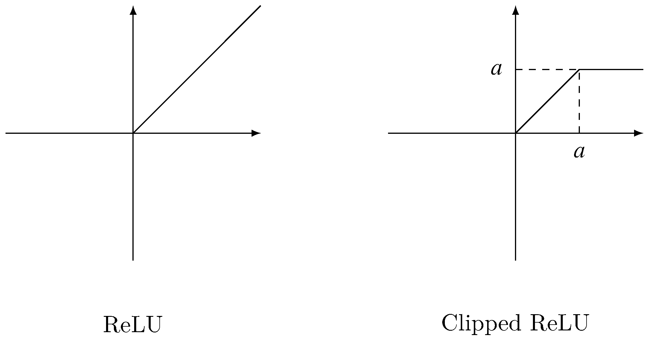
The pre-activation feature maps learned by convolution and BN are then passed through nonlinear activation functions. We introduce two activation functions in the following and compare their effects. Notice that all the operations below are element-wise.

3.3.1. ReLU

ReLU [26] is widely used in deep learning. For the element that greater than 0, it outputs the element itself, for other elements, it outputs 0. Formally, given an input matrix X, the output matrix of ReLU is defined as Equation (8):

$$ReLU\left(X\right)=max\{0,X\}$$

(8)

The left of Figure 3 depicts ReLU activation.

3.3.2. Clipped ReLU

Clipped ReLU is a revision of ReLU. It introduces a parameter $\alpha >0$. Its output for every element that greater than $\alpha$ is $\alpha$. Thus, Clipped ReLU limits the output in $\{0,\alpha \}$. Given an input matrix X, Clipped ReLU is defined as Equation (9):

$$ClippedReLU(X,\alpha )=min\left\{max\right\{0,X\},\alpha \}$$

(9)

The right of Figure 3 depicts Clipped ReLU activation.

3.4. Max Pooling

Above we introduced how to calculate $t_c$ and $windo{w}_c$ for CNN layer without pooling operation. Now we will describe their calculation with a max pooling layer following CNN. Formally, we refer to the time span covered by result element after CNN and max pooling as $t_p$, and the time shift window between two neighbor elements as $windo{w}_p$. For a $w_p\times h_p$ max pooling with pooling strides $s{w}_p\times s{h}_p$, $t_p$ and $windo{w}_p$ can be calculated based on $t_c$ and $windo{w}_c$ as in Equation (10):

$$\begin{array}{cc}\hfill t_p& =t_c+windo{w}_c·(w_p-1)\hfill \\ \hfill windo{w}_p& =s{w}_p·windo{w}_c\hfill \end{array}$$

(10)

Substituting Equations (2) into (10), we can get the final calculating Equations (11) and (12):

$$t_p=t_i+(w_c-1)·windo{w}_i+s{w}_c·windo{w}_i·(w_p-1)$$

(11)

$$windo{w}_p=s{w}_p·s{w}_c·windo{w}_i$$

(12)

Equations (11) and (12) show that max pooling can also enlarge the feature’s corresponding time span and reduce computing steps. Besides, since max pooling uses the maximize value as output, it helps to pick the most important features out from less useful ones.

3.5. Bidirectional LSTM

There are many temporal dependencies in speeches and transcriptions. However, some of them may be so long-term that both CNN and max pooling cannot capture them. Therefore, we use LSTM RNN layer in our model to enable better modeling of the temporal dependencies.

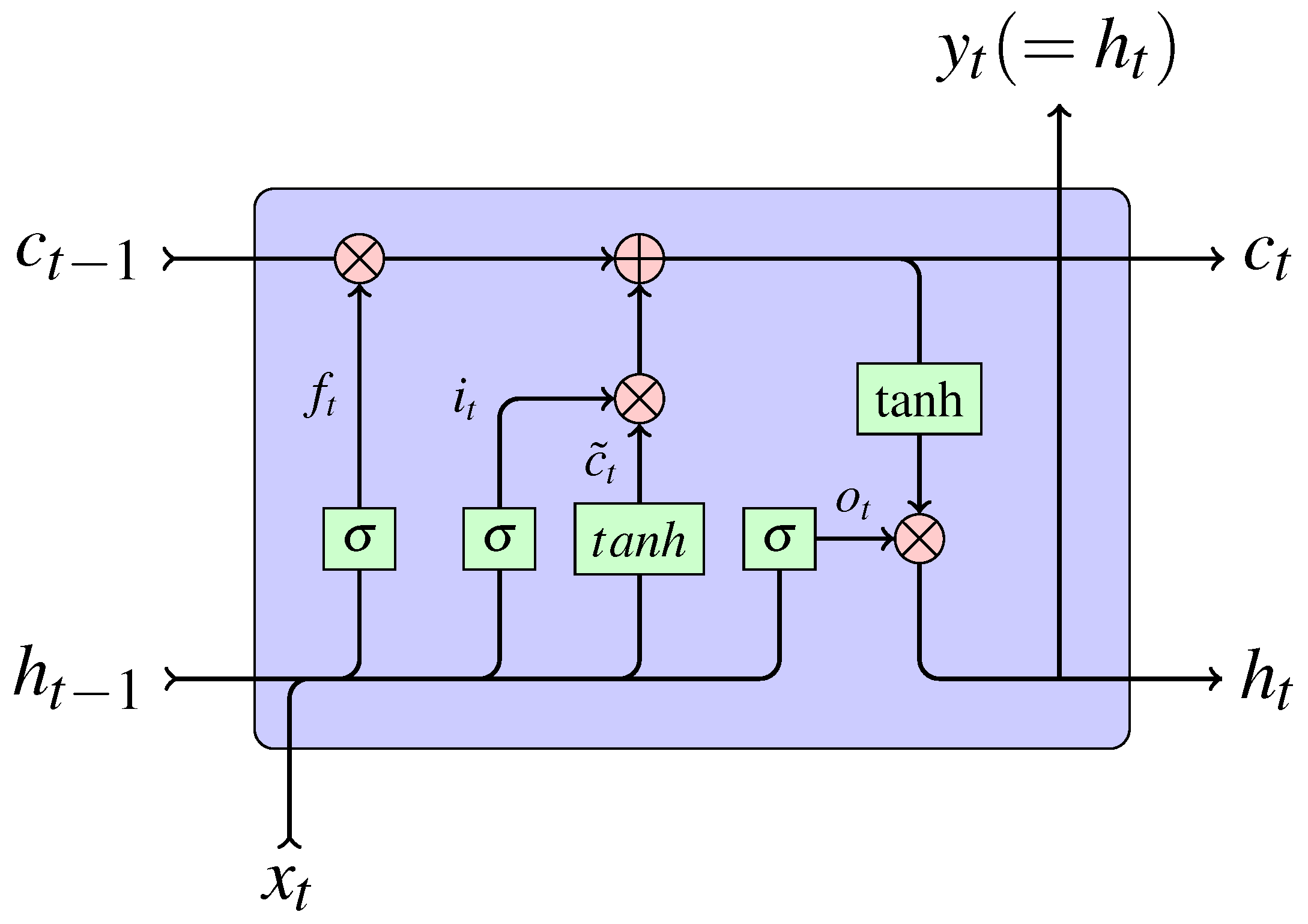
3.5.1. LSTM

The structure of Long-Short Time Memory calculating cell is shown in Figure 4.

At time step t, LSTM uses the following information for calculating:

• $x_t$: input data at current step t.
• $h_{t-1}$: hidden state at previous step $t-1$.
• $c_{t-1}$: cell state at previous step $t-1$.

Given $x_t$, $h_{t-1}$ and $c_{t-1}$, LSTM firstly calculates the forget gate $f_t$ (shown in Equation (13)), the input gate $i_t$ (shown in Equation (14)), the output gate $o_t$ (shown in Equation (15)) and the candidate context ${\tilde{c}}_t$ (shown in Equation (16)).

$$f_t=\sigma ([x_t;h_{t-1}]W_f+b_f)$$

(13)

$$i_t=\sigma ([x_t;h_{t-1}]W_i+b_i)$$

(14)

$$o_t=\sigma ([x_t;h_{t-1}]W_o+b_o)$$

(15)

$${\tilde{c}}_t={\mathcal{F}}_{\tilde{c}}([x_t;h_{t-1}]W_{\tilde{c}}+b_{\tilde{c}})$$

(16)

Then, according to $f_t$, $c_{t-1}$, $i_t$, ${\tilde{c}}_t$, LSTM calculates the cell state $c_t$ at current step as depicted in Equation (17).

$$c_t=f_t{c}_{t-1}+i_t{\tilde{c}}_t$$

(17)

After that, LSTM uses $o_t$ and $c_t$ to calculate the hidden state $h_t$ at current step, which is shown in Equation (18).

$$h_t=o_t\ast {\mathcal{F}}_h\left(c_t\right)$$

(18)

Commonly, ${\mathcal{F}}_{\tilde{c}}(·)$ and ${\mathcal{F}}_h(·)$ are the hyperbolic tangent function.

Finally, LSTM gives its output $y_t$ at time step t, which is same as the hidden state $h_t$.

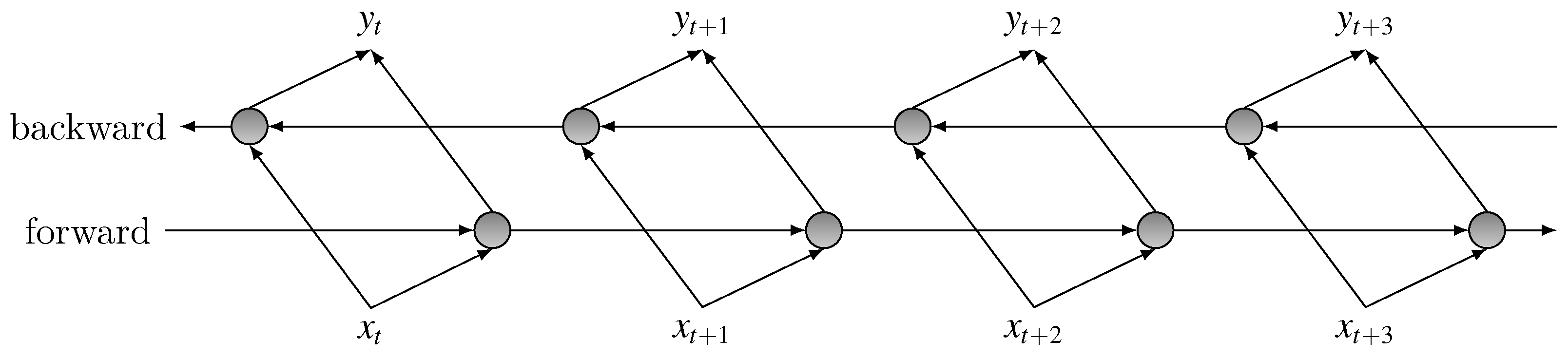
3.5.2. Stacking Up LSTMs of Opposite Directions

However, forward recurrent connection reflects the temporal nature of the audio input, it is typically shown to be beneficial for acoustic models to make full use of the future contextual information [23]. To take advantage of both history and future information from the entire temporal extent of input features, we build a bidirectional LSTM by stacking two opposite LSTM layer, which maintains states both time-forward and time-backward. The structure of BLSTM is demonstrated in Figure 5.

3.6. CTC

Before the proposal of CTC, Some difficulties stand in the way of end-to-end speech recognition. Firstly, the database must be aligned, which is a very exhausting and time-consuming work. This makes it hard to build large-amount database. Secondly, it is a tough process to build a good-performing ASR, because it costs varieties of expertise to design modules such as HMM, CRF, pronunciation lexicons, etc.

By interpreting the network outputs as the probability distributions in possible labels space conditioned on the inputs, CTC addresses these problems properly.

Roughly, CTC can be separated into two procedures: path probability calculating and path merging. In both procedures, the key is that it introduces a new blank label ‘-’ which means no output and an intermediate structure, the path.

For an input sequence $\{x_1,\cdots ,x_T\}$ of length T to CTC, CTC firstly computes a $N+1$ dimension vector at every time step. N is the number of elements in the vocabulary $\mathcal{V}$. Then at each time step i, CTC maps this output vector to the output distribution ${\overrightarrow{p}}_i=\{p_{i,1},\cdots ,p_{i,N+1}\}$ by a SoftMax operation. Here $p_{i,j}(j<N+1)$ is the probability of outputting the j-th elements of the vocabulary at time i, and $p_{i,N+1}$ is the probability of outputting the blank label ‘-’.

After the computation, CTC maps its input sequence $\{x_1,\cdots ,x_T\}$ to a probability sequence $P=\{{\overrightarrow{p}}_1,\cdots ,{\overrightarrow{p}}_T\}$ of the same length T.

If we pick the $w_i$-th element out from set $\mathcal{V}+{\{}^{\prime }{-}^{\prime }\}$ at each time step i and put them together in chronological order, we get a output sequence $\mathcal{P}=\{w_1,\cdots ,w_T\}$ with length T. This $\mathcal{P}$ is a path. This is the definition of path. Since $p_{i,w_i}$ is the probability of output the $w_i$ -th element of $\mathcal{V}+{\{}^{\prime }{-}^{\prime }\}$ at time i, the probability of the path$\mathcal{P}$ can be calculated as Equation (19).

$$P\left(\mathcal{P}\right)=\prod _{i=1}^T{p}_{i,w_i}$$

(19)

Above is the procedure that we called path probability calculating. In this procedure the path is of the same length T as the input sequence, which is not conforming to the actual situations. Commonly the transcription’s length is much shorter than the input sequences. Therefore, we should merge some related paths to a shorter label sequence. This is the path merging procedure. It mainly consists of two operations:

• Remove repeated labels. If there are several same outputs occurring at successive time steps, they are removed and only one of them is kept. E.g., for two different 7-time-step paths ‘c-aa–t-’ and ‘c-a–tt-’, after removing repeated labels, they get the same result sequence ‘c-a-t-’.
• Remove blank label ‘-’ from the path. Now that ‘-’ stands for ‘no output at this step’, it should be removed to get the final label sequence. E.g., the sequence ‘c-a-t-’ becomes ’cat’ after removing all the blank labels.

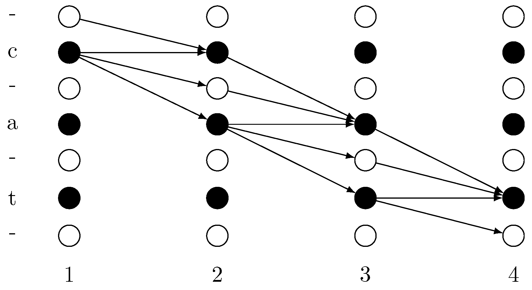
In the merging procedure shown above, ‘c-aa–t-’ and ‘c-a–tt-’ are two paths of length 7, while ‘cat’ is a label sequence of length 3. We can see that a short label sequence may be merged from several long paths. For example, assume the label sequence ’cat’ comes from paths of length 4, then there are 7 different paths included, as shown in Figure 6.

The decoding lattice of these paths are demonstrated in Figure 7. In this figure, 1, 2, 3 and 4 stand for the time step, ‘-’, ‘c’, ‘a’ and ‘t’ stand for the output at each time step. Moving along the arrows’ direction, every path that starts at time step 1 and stops at time step 4 is a legal path for label sequence ‘cat’.

In addition to getting the final label sequence from paths, the path merging procedure also aims to calculating the final label sequence’s probability. For a label sequence L consists of kpaths$\{{\mathcal{P}}_1,\cdots ,{\mathcal{P}}_k\}$, its probability $P\left(L\right)$ is calculated as in Equation (20):

$$P\left(L\right)=\sum _{i=1}^{k}P\left({\mathcal{P}}_i\right)$$

(20)

From the calculation described above we can see that the label sequence’s probability is differentiable. Thus, it enables us to train the model by using back-propagation algorithm to maximize the true label sequence’s probability, and use a trained model to recognize speech by considering the label sequence with the maximize probability as the final result.

4. Experiments and Discussion

4.1. Datasets and Input Features

We train our model completely on the AISHELL-1 corpus, using neither any in-house databases nor external language model. The corpus is divided into training, development, and test set. There are 120,098 utterances from 340 speakers in training set, 14,326 utterances from 40 speakers in development set, and 7176 utterances from 20 speakers in test set. For each speaker, around 360 utterances (about 26 min of speech) are released.

Table 1. Data structure.

Data Set	Durations (h)	Number of Male Speaker	Number of Female Speaker
Training	150	161	179
Development	10	12	28
Test	5	13	7

provides a summary of all subsets in the corpus.

We use MFCC as the model’s input features. It consists of 13-dimensional MFCC with delta and acceleration (in total 39-dimensional features). The MFCC features are derived from the raw audio files with frame window scope of 25 ms and shift window between successive frames of 10ms.

The decoding target vocabulary includes all the 4334 characters (4328 Chinese characters and 6 special tokens ‘ ’, ‘a’, ‘b’, ‘c’, ‘k’, ‘t’) that occurred in the AISHELL-1 transcriptions. Please note that the input of CTC is 4335 (4334 + 1) dimension because the external blank label ‘-’ should be added to the vocabulary when decoding by CTC.

4.2. Convolution Neural Network

Table 2. WERs of models with various CNN depth.

CNN Depth	WER (%)
	Without BLSTM	With BLSTM
2	75.5	26.8
3	71.7	26.4
4	66.7	39.0
5	58.4	44.2
6	60.4	36.4

shows the performance of models with different CNN depth. In these models every CNN layer has 64 feature maps. In the table numbers in bold give the best WERs of every group of models respectively.

For models without BLSTM (there are only CNN and full connected layers), model’s performance increases as we deepen the CNN layers from 2 to 5. However, deeper CNN does not necessarily lead to better performance, as the model with 6 CNN layers has a higher WER than the model with 5 CNN layers.

When we deepen the CNN, model performance first increases. It shows that local contextual features play a significant role for speech recognition. Deeper CNN can learn local features of a longer time scope and a larger frequency scope. It enables the model to use more local information to determine the output at current step.

However, this positive effect does not always exist. When the local context covers too large scope (for the model without BLSTM, when the CNN is deeper than with 5 layers), it introduces too much unnecessary information that it dulls those really distinct features, and results in a worse performance.

As shown in the third column in Table 2, this phenomenon also exists in the model using BLSTM. However, since the BLSTM can model contextual information itself, the turning of performance increasing to decreasing comes early (only with 3 CNN layers, rather than 5).

We find that this phenomenon of performance firstly increasing and then decreasing has something to do with the speaking speed. In this experiments, for CNNs from the first layer to the sixth, the kernels are $3\times 2$, $2\times 2$, $2\times 2$, $2\times 2$, $2\times 1$, $2\times 1$, convolution strides are all $1\times 1$. For max pooling from the first layer to the fourth (there is no higher max pooling layer), their pooling sizes are $2\times 2$, $2\times 2$, $2\times 2$, $2\times 1$, and pooling strides are $2\times 2$, $2\times 1$, $2\times 1$, $2\times 1$. Given that every MFCC frame’s time scope is 25 ms, shift window is 10 ms, calculated as described in Section 3.4, we know that the fifth CNN layer covers a time scope of 335 ms, while the fourth layer covers a much smaller scope (175 ms) and the sixth layer covers a much larger scope (495 ms). We then analyze the datasets and find that the speaking speeds of training, development, and test, and the total AISHELL-1 dataset are 3.2, 3.1, 2.9 and 3.2 characters per second, respectively. This means that in the dataset, every character corresponds to an audio piece lasting for about 300 ms. This is consistent with the fifth layer’s time scope.

4.3. Bidirectional LSTM

Table 2 also compares models with and without BLSTM. Every line in Table 2 reveals that the model using BLSTM outperforms that using no BLSTM significantly. It may because BLSTM’s ability of modeling contextual information is much stronger than CNN. At each time step, BLSTM uses forget gate to determine how much history information should be kept, and uses input gate to determine how much new information should be added. Since all the gates are derived from previous hidden state and current input, BLSTM can set different weights for different location when computing contextual information at different time. Besides, by setting far-away location’s weights to 0 (or nearly 0), BLSTM can dynamically determine the context span. In addition, and more important than that, BLSTM can model contextual information from both forward and backward direction. All these together enables BLSTM surpassing CNNs.

In previous experiments, the number of hidden units in BLSTM is 128. For BLSTM, its number of hidden units is very influential for performance. Different number of hidden units means that the BLSTM uses features of different dimension to model the contextual information and current input. It cannot work properly with low dimension. However, too high dimension may introduce unnecessary feature patterns which will confuse the recognition model. So it is important to set the number of hidden units properly.

Performance of models with different hidden dimension are given in

Table 3. Comparison of Models with different number of hidden units in BLSTM.

Number of Hidden Units	WER (%)
128	26.4
256	23.7
384	23.6
512	21.2
640	21.0
768	19.2
896	20.0

. Number in bold is the best WER. Model performance increases as we enlarge the hidden dimension from 128 to 768, and achieves the best WER of 19.2% with a hidden dimension of 768. However, when we enlarge the hidden dimension from 768 to 896, the performance begins to decrease. We think this is because 896 is a too high dimension for the model and it introduces unnecessary feature patterns which confuses the recognition model. As a result, the WER increases.

Many works use more than one RNN layers in ASR. For example, DeepSpeech2 uses 5 RNN layers. We conduct experiments to compare the performance of models with different BLSTM depth, results are given in

Table 4. Comparison of models with different BLSTM depth.

Depth of BLSTM	WER (%)
1	19.2
2	25.8

. The bold number in this table is the best WER.

Model with 2 BLSTM layers performs even worse than that with only 1 BLSTM layer. BLSTM can model contextual information from two directions. Results in Table 2 show that one-BLSTM model can learn contextual information sufficiently (because it reduces CNN layers from 5 to 3 and achieves the best WER). Therefore, using more BLSTM only unnecessarily enlarges context scope and involves more useless features, which confuses the model and pulls the performance down.

Commonly, results of the two opposite-direction LSTM are concatenated along the time dimension as the input for subsequent neural layers. Nevertheless, there are some works adding them up instead of concatenating. Since the adding operation may counteract the opposite-direction features and make it difficult to distinguish them, we think the concatenation may achieves better results than adding them up. Experiments results in

Table 5. Comparison of models using concatenation and addition.

Model	WER (%)
concatenate	19.2
add	29.0

verify this analysis. The bold number in this table is the best WER.

4.4. Batch Normalization

BN uses the average and variance of training dataset for recognition on test dataset. Thus, objectively it requires training, and testing dataset have the same average and variance. Otherwise it may fail to improve the performance.

Since the AISHELL-1 is not a very large corpus (it contains 170 h speech, while some English corpus contains tens of thousands of hours of speech data), the training and testing sets may have different distributions. we compare models with and without BN to verify BN’s effect. Results are given in

Table 6. Comparison of Batch Normalization’s effect.

Model	WER (%)
with BN	19.2
without BN	30.7

, where the bold number gives the best WER. They show that BN can improve the CNN+BLSTM+CTC model on AISHELL-1 corpus remarkably.

4.5. Activations

Activation functions also impact model’s performance significantly. Many of recent outstanding works use Clipped ReLU activation $\mathcal{F}(x,\alpha )=min\left\{max\right\{x,0\},\alpha \}$ [1,9,10,14]. More than that, some of them set $\alpha =20$ [1,9,14].

However, at the same time, there are still many works using the ReLU activation $\mathcal{F}\left(x\right)=max\{x,0\}$ [7,19,22,23,24,27,28].

We conduct experiments to compare these two activation functions, results are shown in

Table 7. Effect of different Activations.

Activation	WER (%)
ReLU	19.2
Clipped ReLU	27.5

. For our model on AISHELL-1 dataset, the ReLU activation gives better performance.

4.6. Comparison with Existing Works

We compare our work with two existing works: CNN-input [6] and ACS [7]. CNN-input [6] achieves WER of 20.68% on the AISHELL-1 data without language model. In [7], the ACS method gets CER of 21.6% on AISHELL-1 test without language model, while adding bidirectional contexts and RNN language model (referred to as ACS+Bidirectional Contexts+RNN-LM), the CER drops to 18.7%. The comparison is shown in

Table 8. Comparison with existing works.

Model	WER (%)
CNN-input [6]	20.68
ACS [7]	21.6
CNN+BLSTM+CTC	19.2

, where the best WER is given in bold. Our model CNN+BLSTM+CTC achieves the best performance.

5. Conclusions

There are many difficulties to build and train conventional ASR systems, since such systems contain many sub-modules and need lots of domain knowledge. However, as to end-to-end Mandarin ASR systems, most of them are neither reproducible nor comparable because they use specific language model and in-house training database which are not freely available.

In this paper, we propose a CNN+BLSTM+CTC end-to-end Mandarin ASR. The CNN+BLSTM+CTC ASR uses CNN to learn local speech features, uses BLSTM to learn history and future contextual information. It is trained completely on the by-far-largest open-source Mandarin speech corpus AISHELL-1, using neither any in-house database nor external language model. It achieves a WER of 19.2%, outperforming the exiting best work. Now that all data corpora we used are freely available, our model is reproducible and comparable, providing a new baseline for further Mandarin ASR research.

6. Future Works

Although our work achieves a good performance, there are still some future works to do.

• We use MFCC as the input features. However, for English ASR, there are works using original wav signals, spectrogram, and other acoustic features as input. For Mandarin speech recognition, modeling units of acoustic model also affect the performance significantly [29]. We will compare their differences and find the best input acoustic features for Mandarin ASR.
• Bidirectional LSTM suffers from long latency, so it does not suit the online ASR scenario. We will explore unidirectional LSTM or other techniques to shorten the latency.
• Language model is crucial for ASR, and [12] shows that with enough speech transcriptions, end-to-end ASR can learn language model implicitly. Therefore, another future work is to explore language model and develop end-to-end Mandarin ASR on some larger databases.