Some Symmetric Identities for the Multiple (p, q)-Hurwitz-Euler eta Function

Abstract

The main purpose of this paper is to find some interesting symmetric identities for the $(p,q)$-Hurwitz-Euler eta function in a complex field. Firstly, we define the multiple $(p,q)$-Hurwitz-Euler eta function by generalizing the Carlitz’s form $(p,q)$-Euler numbers and polynomials. We find some formulas and properties involved in Carlitz’s form $(p,q)$-Euler numbers and polynomials with higher order. We find new symmetric identities for multiple $(p,q)$-Hurwitz-Euler eta functions. We also obtain symmetric identities for Carlitz’s form $(p,q)$-Euler numbers and polynomials with higher order by using symmetry about multiple $(p,q)$-Hurwitz-Euler eta functions. Finally, we study the distribution and symmetric properties of the zero of Carlitz’s form $(p,q)$-Euler numbers and polynomials with higher order.

1. Introduction

The area of the specific functions like the gamma and beta functions, the hypergeometric functions, special polynomials, the zeta functions and the area of series such as q-series, and series representations are a rapidly developing area in advanced mathematics (see [1,2,3,4,5,6,7,8,9,10,11,12,13,14,15]). Many q-extensions of specific functions and polynomials have been studied (see [1,3,6,7,8,9,10,13,16]). Srivastava [15] discussed some properties and q-extensions of the Bernoulli polynomials, Euler polynomials, and Genocchi polynomials. Choi, Anderson and Srivastava have developed the q-extension of the Riemann zeta function and functions related to the Riemann zeta function (see [5]). Choi and Srivastava presented a generalized Hurwitz formula and Hurwitz-Euler eta function (see [4]). Recently, many authors have developed $(p,q)$-extensions of the special functions, Riemann zeta function and related functions (see [1,13,17,18,19]). The symmetry of special polynomials is also actively studied (see [8,9,19]).

We use this

$$\sum _{m_1=0}^n\cdots \sum _{m_r=0}^n=\sum _{m_1,\cdots ,m_r=0}^n.$$

We know the binomial formula as

$${(1-a)}^n=\sum _{i=0}^n\left(\genfrac{}{}{0pt}{}{n}{i}\right){(-a)}^i,\mathrm{where}\left(\genfrac{}{}{0pt}{}{n}{i}\right)={\displaystyle \frac{n(n-1)\cdots (n-i+1)}{i!}},$$

and

$${\displaystyle \frac{1}{{(1-a)}^n}}={(1-a)}^{-n}=\sum _{i=0}^{\infty }\left(\genfrac{}{}{0pt}{}{-n}{i}\right){(-a)}^i=\sum _{i=0}^{\infty }\left(\genfrac{}{}{0pt}{}{n+i-1}{i}\right)a^i.$$

Choi and Srivastava [4] constructed and made formulas about the multiple Hurwitz-Euler eta function ${\eta }_r(s,a)$ defined by following r-ple series:

$${\eta }_r(s,a)=\sum _{k_1,\cdots ,k_r=0}^{\infty }{\displaystyle \frac{{(-1)}^{k_1+\cdots +k_r}}{{(k_1+\cdots +k_r+a)}^s}},(Re\left(s\right)>0;a>0;r\in \mathbb{N}),$$

where $\mathbb{N}$ is the set of natural numbers. It is known that ${\eta }_r(s,a)$ can be analytically continued to be all complex s-plane (see [4]). The $(p,q)$-number was defined as

$${\left[n\right]}_{p,q}=\frac{p^n-q^n}{p-q}=p^{n-1}+p^{n-2}q+p^{n-3}{q}^2+\cdots +p^2{q}^{n-3}+p{q}^{n-2}+q^{n-1}.$$

It can be seen that the $(p,q)$-number contains a symmetric property, and this number is q-number when $p=1$. In particular, we can see ${lim}_{q\to 1}{\left[n\right]}_{p,q}=n$ with $p=1$. Since ${\left[n\right]}_{p,q}=p^{n-1}{\left[n\right]}_{\frac{q}{p}}$, we observe that p-numbers and $(p,q)$-numbers are different. In other words, by substituting q by $\frac{q}{p}$ in the q-number, we could not obtain a $(p,q)$-number. Therefore, much research has been conducted in the area of special functions by using $(p,q)$-number (see [1,13,18,19]). In this article, the $(p,q)$-extension of the multiple form of Hurwitz-Euler eta function can be defined as follows: For $s,x\in \mathbb{C}$ with $Re\left(x\right)>0$, the multiple $(p,q)$-Hurwitz-Euler eta function ${\eta }_{p,q}^{\left(r\right)}(s,x)$ is defined by

$${\eta }_{p,q}^{\left(r\right)}(s,x)={\left[2\right]}_q^r\sum _{m_1,\dots ,m_r=0}^{\infty }{\displaystyle \frac{{(-1)}^{m_1+\cdots +m_r}{q}^{m_1+\cdots +m_r}}{{[m_1+\cdots +m_r+x]}_{p,q}^s}}.$$

The aim of this paper is to introduce and study a new some generalizations of the Carlitz’s form higher order q-Euler numbers and polynomials, the multiple q-Euler zeta function, and the multiple Hurwitz q-Euler zeta function. We call them Carlitz’s type higher-order $(p,q)$-Euler numbers and polynomials, the multiple $(p,q)$-Euler zeta function, and the multiple $(p,q)$-Hurwitz-Euler eta function. The paper is structured as follows. In Section 2 we define Carlitz’s type higher-order $(p,q)$-Euler numbers and $(p,q)$-Euler polynomials and induce some of their properties involving elementary properties, distribution relation, property of complement, and so on. In Section 3, by using the Carlitz’s type higher-order $(p,q)$-Euler numbers and polynomials, the multiple $(p,q)$-Euler zeta function and the multiple $(p,q)$-Hurwitz-Euler eta function are defined. We also present some connection formulae between the Carlitz’s type higher-order $(p,q)$-Euler numbers and polynomials, the multiple $(p,q)$-Euler zeta function, and the multiple $(p,q)$-Hurwitz-Euler eta function. In Section 4 we give several symmetric identities about the multiple $(p,q)$-Hurwitz-Euler eta function and Carlitz’s type higher-order $(p,q)$-Euler numbers and polynomials. In Section 5, we investigate the distribution and symmetry of the zero of Carlitz’s type higher-order $(p,q)$-Euler polynomials using a computer. Our paper ends with Section 6, where the conclusions and future developments of this work are presented.

Definition 1.

The classical higher-order Euler numbers denoted by $E_n^{\left(r\right)}$ and Euler polynomials denoted by $E_n^{\left(r\right)}\left(x\right)$ are defined as the below generating functions

$${\left({\displaystyle \frac{2}{e^t+1}}\right)}^r=\sum _{n=0}^{\infty }{E}_n^{\left(r\right)}\frac{t^n}{n!},\left(\right|t|<\pi ),$$

and

$${\left({\displaystyle \frac{2}{e^t+1}}\right)}^r{e}^{xt}=\sum _{n=0}^{\infty }{E}_n^{\left(r\right)}\left(x\right)\frac{t^n}{n!},\left(\right|t|<\pi ),$$

respectively (see [15]).

Definition 2.

For $0<q<p\le 1$, the Carlitz’s type $(p,q)$-Euler polynomials denoted by $E_{n,p,q}\left(x\right)$ are defined as the below generating function (see [13])

$$\sum _{n=0}^{\infty }{E}_{n,p,q}\left(x\right)\frac{t^n}{n!}={\left[2\right]}_q\sum _{m=0}^{\infty }{(-1)}^m{q}^m{e}^{{[m+x]}_{p,q}t}.$$

2. Carlitz’s Form Higher-Order $(\mathit{p},\mathit{q})$-Euler Numbers and Polynomials

First, we think the Carlitz’s form with high-order $(p,q)$-Euler numbers and polynomials as follows:

Definition 3.

For $r\in \mathbb{N}$, the high-order $(p,q)$-Euler polynomials denoted by $E_{n,p,q}^{\left(r\right)}\left(x\right)$ are defined like the generating function:

$$\sum _{n=0}^{\infty }{E}_{n,p,q}^{\left(r\right)}\left(x\right){\displaystyle \frac{t^n}{n!}}={\left[2\right]}_q^r\sum _{m_1,\cdots ,m_r=0}^{\infty }{(-1)}^{m_1+\cdots +m_r}{q}^{m_1+\cdots +m_r}{e}^{{[m_1+\cdots +m_r+x]}_{p,q}t}.$$

(1)

If $x=0,E_{n,p,q}^{\left(r\right)}=E_{n,p,q}^{\left(r\right)}\left(0\right)$ are called the higher-order $(p,q)$-Euler numbers $E_{n,p,q}^{\left(r\right)}$. Note that if $r=1$, then $E_{n,p,q}^{\left(r\right)}=E_{n,p,q}$ and $E_{n,p,q}^{\left(r\right)}\left(x\right)=E_{n,p,q}\left(x\right)$. Observe that if $p=1,q\to 1$, then $E_{n,p,q}^{\left(r\right)}\to E_n^{\left(r\right)}$ and $E_{n,p,q}^{\left(r\right)}\left(x\right)\to E_n^{\left(r\right)}\left(x\right)$.

Definition 4.

For $r\in \mathbb{N}$, the $(h,p,q)$-Euler polynomials with high-order denoted by $E_{n,p,q}^{(r,h)}\left(x\right)$ are defined as the below generating function:

$${\displaystyle \sum _{n=0}^{\infty }}{E}_{n,p,q}^{(r,h)}\left(x\right){\displaystyle \frac{t^n}{n!}}={\left[2\right]}_q^r{\displaystyle \sum _{m_1,\cdots ,m_r=0}^{\infty }}{(-q)}^{m_1+\cdots +m_r}{p}^{h(m_1+\cdots +m_r)}{e}^{{[m_1+\cdots +m_r+x]}_{p,q}t}.$$

(2)

If $x=0,E_{n,p,q}^{(r,h)}=E_{n,p,q}^{(r,h)}\left(0\right)$ is called $(h,p,q)$-Euler numbers with higher-order denoted by $E_{n,p,q}^{\left(r\right)}$. Remark that if $h=0$, then $E_{n,p,q}^{(r,h)}=E_{n,p,q}^{\left(r\right)}$ and $E_{n,p,q}^{(r,h)}\left(x\right)=E_{n,p,q}^{\left(r\right)}\left(x\right)$. We see that if $r=1$, then $E_{n,p,q}^{(r,h)}=E_{n,p,q}^{\left(h\right)}$ and $E_{n,p,q}^{(r,h)}\left(x\right)=E_{n,p,q}^{\left(h\right)}\left(x\right)$ (see [13]). Observe that if $p=1,q\to 1$, then $E_{n,p,q}^{(r,h)}\to E_n^{\left(r\right)}$ and $E_{n,p,q}^{(r,h)}\left(x\right)\to E_n^{\left(r\right)}\left(x\right)$.

By (1) and (2), we know that

$$\begin{array}{l}{E}_{n,p,q}^{\left(r\right)}(x+y)={\displaystyle \sum _{i=0}^n}\left(\genfrac{}{}{0pt}{}{n}{i}\right)p^{(n-i)x}{q}^{yi}{E}_{i,p,q}^{(r,n-i)}\left(x\right){\left[y\right]}_{p,q}^{n-i},\\ E_{n,p,q}^{\left(r\right)}\left(x\right)={\displaystyle \sum _{i=0}^n}\left(\genfrac{}{}{0pt}{}{n}{i}\right)q^{xi}{\left[x\right]}_{p,q}^{n-i}{E}_{i,p,q}^{(r,n-i)}.\end{array}$$

(3)

Theorem 1.

For $r\in \mathbb{N}$, we have

$$\begin{array}{cc}\hfill E_{n,p,q}^{\left(r\right)}\left(x\right)& ={\left[2\right]}_q^r{\displaystyle \sum _{m_1,\cdots ,m_r=0}^{\infty }}{(-1)}^{m_1+\cdots +m_r}{q}^{m_1+\cdots +m_r}{[m_1+\cdots +m_r+x]}_{p,q}^n\hfill \\ \hfill & ={\displaystyle \frac{{\left[2\right]}_q^r}{{(p-q)}^n}}{\displaystyle \sum _{l=0}^n}\left(\genfrac{}{}{0pt}{}{n}{l}\right){(-1)}^l{q}^{xl}{p}^{(n-l)x}{\left({\displaystyle \frac{1}{1+q^{l+1}{p}^{n-l}}}\right)}^r.\hfill \end{array}$$

Proof. 

When we use the Taylor series expansion of $e^{{\left[x\right]}_{p,q}t}$, we can get

$$\begin{array}{cc}\hfill {\displaystyle \sum _{l=0}^{\infty }}{E}_{l,p,q}^{\left(r\right)}\left(x\right){\displaystyle \frac{t^l}{l!}}=& {\left[2\right]}_q^r{\displaystyle \sum _{m_1,\cdots ,m_r=0}^{\infty }}{(-1)}^{m_1+\cdots +m_r}{q}^{m_1+\cdots +m_r}{e}^{{[m_1+\cdots +m_r+x]}_{p,q}t}\hfill \\ \hfill & ={\displaystyle \sum _{l=0}^{\infty }}\left({\left[2\right]}_q^r{\displaystyle \sum _{m_1,\cdots ,m_r=0}^{\infty }}{(-1)}^{m_1+\cdots +m_r}{q}^{m_1+\cdots +m_r}{[m_1+\cdots +m_r+x]}_{p,q}^l\right){\displaystyle \frac{t^l}{l!}}.\hfill \end{array}$$

The first part of the theorem follows when we compare the coefficients of $\frac{t^l}{l!}$ in the above equation. By $(p,q)$-numbers and binomial expansion, we also note that

$$\begin{array}{cc}\hfill E_{n,p,q}^{\left(r\right)}\left(x\right)& ={\left[2\right]}_q^r{\displaystyle \sum _{m_1,\cdots ,m_r=0}^{\infty }}{(-1)}^{m_1+\cdots +m_r}{q}^{m_1+\cdots +m_r}{[m_1+\cdots +m_r+x]}_{p,q}^n\hfill \\ \hfill & ={\left[2\right]}_q^r{\displaystyle \sum _{m_1,\cdots ,m_r=0}^{\infty }}{(-1)}^{m_1+\cdots +m_r}{q}^{m_1+\cdots +m_r}{\left({\displaystyle \frac{p^{m_1+\cdots +m_r+x}-q^{m_1+\cdots +m_r+x}}{p-q}}\right)}^n\hfill \\ \hfill & ={\displaystyle \frac{{\left[2\right]}_q^r}{{(p-q)}^n}}{\displaystyle \sum _{l=0}^n}\left(\genfrac{}{}{0pt}{}{n}{l}\right){(-1)}^l{q}^{xl}{p}^{(n-l)x}\hfill \\ \hfill & \times {\displaystyle \sum _{m_1,\cdots ,m_r=0}^{\infty }}{(-1)}^{m_1+\cdots +m_r}{q}^{(l+1)(m_1+\cdots +m_r)}{p}^{(n-l)(m_1+\cdots +m_r)}\hfill \\ \hfill & ={\displaystyle \frac{{\left[2\right]}_q^r}{{(p-q)}^n}}{\displaystyle \sum _{l=0}^n}\left(\genfrac{}{}{0pt}{}{n}{l}\right){(-1)}^l{q}^{xl}{p}^{(n-l)x}{\left({\displaystyle \frac{1}{1+q^{l+1}{p}^{n-l}}}\right)}^r.\hfill \end{array}$$

We finish the proof of Theorem 1. □

Theorem 2.

For $r\in \mathbb{N}$, we get

$$E_{n,p,q}^{\left(r\right)}\left(x\right)={\left[2\right]}_q^r\sum _{m=0}^{\infty }\left(\genfrac{}{}{0pt}{}{r+m-1}{m}\right){(-1)}^m{q}^m{[m+x]}_{p,q}^n.$$

(4)

Proof. 

By Taylor-Maclaurin series expansion of ${(1-a)}^{-n}$, we have

$${\left({\displaystyle \frac{1}{1+q^{l+1}{p}^{n-l}}}\right)}^r=\sum _{m=0}^{\infty }\left(\genfrac{}{}{0pt}{}{m+r-1}{m}\right){(-1)}^m{\left(q^{l+1}{p}^{n-l}\right)}^m.$$

Also, by Theorem 1 and binomial expansion, one can obtain the desired result immediately. □

For $d\in \mathbb{N}$ with $d\equiv 1\left(\mathrm{mod}2\right)$, by Theorem 1 we can show

$$\begin{array}{cc}\hfill E_{n,p,q}^{\left(r\right)}\left(x\right)=& {\displaystyle \frac{{\left[2\right]}_q^r}{{(p-q)}^n}}{\displaystyle \sum _{l=0}^n}\left(\genfrac{}{}{0pt}{}{n}{l}\right){(-1)}^l{q}^{xl}{p}^{(n-l)x}{\displaystyle \sum _{a_1,\cdots ,a_r=0}^{d-1}}{\displaystyle \sum _{m_1,\cdots ,m_r=0}^{\infty }}{(-1)}^{a_1+\cdots +a_r}\hfill \\ \hfill & \times {(-1)}^{m_1+\cdots +m_r}{q}^{(l+1)(a_1+d{m}_1+\cdots +a_r+d{m}_r)}{p}^{(n-l)(a_1+d{m}_1+\cdots +a_r+d{m}_r)}.\hfill \end{array}$$

Theorem 3.

(Distribution relation of $(p,q)$-Euler polynomials with higher-order). For $d\in \mathbb{N}$ with $d\equiv 1\left(mod2\right)$, we have

$$E_{n,p,q}^{\left(r\right)}\left(x\right)={\displaystyle \frac{{\left[2\right]}_q^r}{{\left[2\right]}_{q^d}^r}}{\left[d\right]}_{p,q}^n\sum _{a_1,\cdots ,a_r=0}^{d-1}{(-q)}^{a_1+\cdots +a_r}{E}_{n,p^d,q^d}^{\left(r\right)}\left({\displaystyle \frac{a_1+\cdots +a_r+x}{d}}\right).$$

Proof. 

Since

$$\begin{array}{l}{E}_{n,p^d,q^d}^{\left(r\right)}\left({\displaystyle \frac{a_1+\cdots +a_r+x}{d}}\right)\\ ={\displaystyle \frac{{\left[2\right]}_{q^d}^r}{{(p^d-q^d)}^n}}{\displaystyle \sum _{l=0}^n}\left(\genfrac{}{}{0pt}{}{n}{l}\right){(-1)}^l{q}^{l(a_1+\cdots +a_r+x)}{p}^{(n-l)(a_1+\cdots +a_r+x)}{\left({\displaystyle \frac{1}{1+q^{d(l+1)}{p}^{d(n-l)}}}\right)}^r,\end{array}$$

we have

$$\begin{array}{l}{\displaystyle \sum _{a_1,\cdots ,a_r=0}^{d-1}}{(-q)}^{a_1+\cdots +a_r}{E}_{n,p^d,q^d}^{\left(r\right)}\left({\displaystyle \frac{a_1+\cdots +a_r+x}{d}}\right)\\ ={\displaystyle \frac{{\left[2\right]}_{q^d}^r}{{(p^d-q^d)}^n}}{\displaystyle \sum _{l=0}^n}\left(\genfrac{}{}{0pt}{}{n}{l}\right){(-1)}^l{q}^{lx}{p}^{(n-l)x}\\ \times {\displaystyle \sum _{a_1,\cdots ,a_r=0}^{d-1}}{(-1)}^{a_1+\cdots +a_r}{q}^{a_1+\cdots +a_r}{q}^{l(a_1+\cdots +a_r)}{p}^{(n-l)(a_1+\cdots +a_r)}{\left({\displaystyle \frac{1}{1+q^{d(l+1)}{p}^{d(n-l)}}}\right)}^r.\end{array}$$

Hence, we derive

$$\begin{array}{l}{\displaystyle \frac{{\left[2\right]}_q^r}{{\left[2\right]}_{q^d}^r}}{\left[d\right]}_{p,q}^n{\displaystyle \sum _{a_1,\cdots ,a_r=0}^{d-1}}{(-q)}^{a_1+\cdots +a_r}{E}_{n,p^d,q^d}^{\left(r\right)}\left({\displaystyle \frac{a_1+\cdots +a_r+x}{d}}\right)\\ ={\displaystyle \frac{{\left[2\right]}_q^r}{{(p-q)}^n}}{\displaystyle \sum _{l=0}^n}\left(\genfrac{}{}{0pt}{}{n}{l}\right){(-1)}^l{q}^{xl}{p}^{(n-l)x}{\left({\displaystyle \frac{1}{1+q^{l+1}{p}^{n-l}}}\right)}^r.\end{array}$$

We prove Theorem 3. □

3. Multiple $(\mathit{p},\mathit{q})$-Hurwitz-Euler eta Function

We define multiple $(p,q)$-Hurwitz-Euler eta function. This function makes $(p,q)$-Euler polynomials at negative integers with higher-order. Choi and Srivastava [4] defined ${\eta }_r(s,a)$ by means of

$${\eta }_r(s,a)=\sum _{k_1,\cdots ,k_r=0}^{\infty }{\displaystyle \frac{{(-1)}^{k_1+\cdots +k_r}}{{(k_1+\cdots +k_r+a)}^s}},(Re\left(s\right)>0;a>0;r\in \mathbb{N}).$$

It is known that ${\eta }_r(s,a)$ can be continued analytically to be all complex s-plane (see [4]). The $(p,q)$-extension of ${\eta }_r(s,a)$ can be defined as follows:

Definition 5.

For $s,x\in \mathbb{C}$ with $Re\left(x\right)>0$, the multiple $(p,q)$-Hurwitz-Euler eta function ${\eta }_{p,q}^{\left(r\right)}(s,x)$ is defined as

$${\eta }_{p,q}^{\left(r\right)}(s,x)={\left[2\right]}_q^r\sum _{m_1,\dots ,m_r=0}^{\infty }{\displaystyle \frac{{(-1)}^{m_1+\cdots +m_r}{q}^{m_1+\cdots +m_r}}{{[m_1+\cdots +m_r+x]}_{p,q}^s}}.$$

Observe that when $p=1,q\to 1$, then $2^r{\eta }_{p,q}^{\left(r\right)}(s,a)={\eta }_r(s,a)$.

Let

$$\begin{array}{cc}\hfill F_{p,q}^{\left(r\right)}(t,x)& {\displaystyle =\sum _{n=0}^{\infty }}{E}_{n,p,q}^{\left(r\right)}\left(x\right){\displaystyle \frac{t^n}{n!}}\hfill \\ \hfill & ={\left[2\right]}_q^r{\displaystyle \sum _{m_1,\dots ,m_r=0}^{\infty }}{(-1)}^{m_1+\cdots +m_r}{q}^{m_1+\cdots +m_r}{e}^{{[m_1+\cdots +m_r+x]}_{p,q}t}.\hfill \end{array}$$

(5)

Theorem 4.

For $r\in \mathbb{N}$, we get

$${\eta }_{p,q}^{\left(r\right)}(s,x)={\displaystyle \frac{1}{\mathsf{\Gamma }\left(s\right)}}{\int }_0^{\infty }{F}_{p,q}^{\left(r\right)}(x,-t)t^{s-1}dt,$$

(6)

where $\mathsf{\Gamma }\left(s\right)={\int }_0^{\infty }{z}^{s-1}{e}^{-z}dz$.

Proof. 

From (5) and Definition 5, we get

$$\begin{array}{cc}\hfill {\eta }_{p,q}^{\left(r\right)}(s,x)& ={\left[2\right]}_q^r{\displaystyle \sum _{m_1,\cdots ,m_r=0}^{\infty }}{\displaystyle \frac{{(-1)}^{m_1+\cdots +m_r}{q}^{m_1+\cdots +m_r}}{{[m_1+\cdots +m_r+x]}_{p,q}^s}}\hfill \\ \hfill & ={\left[2\right]}_q^r{\displaystyle \frac{1}{\mathsf{\Gamma }\left(s\right)}}{\displaystyle \sum _{m_1,\cdots ,m_r=0}^{\infty }}{\displaystyle \frac{{(-1)}^{m_1+\cdots +m_r}{q}^{m_1+\cdots +m_r}}{{[m_1+\cdots +m_r+x]}_{p,q}^s}}{\int }_0^{\infty }{z}^{s-1}{e}^{-z}dz\hfill \\ \hfill & ={\displaystyle \frac{{\left[2\right]}_q^r}{\mathsf{\Gamma }\left(s\right)}}{\displaystyle \sum _{m_1,\cdots ,m_r=0}^{\infty }}{(-1)}^{m_1+\cdots +m_r}{q}^{m_1+\cdots +m_r}{\int }_0^{\infty }{e}^{{[m_1+\cdots +m_r+x]}_{p,q}t}{t}^{s-1}dt\hfill \\ \hfill & ={\displaystyle \frac{1}{\mathsf{\Gamma }\left(s\right)}}{\int }_0^{\infty }{F}_{p,q}^{\left(r\right)}(x,-t)t^{s-1}dt.\hfill \end{array}$$

We are finished Theorem 4. □

The value of multiple $(p,q)$-Hurwitz-Euler eta function ${\eta }_{p,q}^{\left(r\right)}(s,x)$ at negative integers is given explicitly by the following theorem:

Theorem 5.

Let $n\in N$. Then we obtain

$${\eta }_{p,q}^{\left(r\right)}(-n,x)=E_{n,p,q}^{\left(r\right)}\left(x\right).$$

Proof. 

Again, by (5) and (6), we have

$${\eta }_{p,q}^{\left(r\right)}(s,x)={\displaystyle \frac{1}{\mathsf{\Gamma }\left(s\right)}}{\int }_0^{\infty }{F}_{p,q}^{\left(r\right)}(x,-t)t^{s-1}dt={\displaystyle \frac{1}{\mathsf{\Gamma }\left(s\right)}}\sum _{m=0}^{\infty }{E}_{m,p,q}^{\left(r\right)}\left(x\right){\displaystyle \frac{{(-1)}^m}{m!}}{\int }_0^{\infty }{t}^{m+s-1}dt.$$

(7)

We note that

$$\mathsf{\Gamma }(-n)={\int }_0^{\infty }{e}^{-z}{z}^{-n-1}dz={\displaystyle \underset{z\to 0}{lim}}2\pi i\frac{1}{n!}{\left(\frac{d}{dz}\right)}^n\left(z^{n+1}{e}^{-z}{z}^{-n-1}\right)=2\pi i\frac{{(-1)}^n}{n!}.$$

(8)

For $n\in \mathbb{N}$, let us take $s=-n$ in (7). Then, by (7), (8), and Cauchy residue theorem, we have

$$\begin{array}{cc}\hfill {\eta }_{p,q}^{\left(r\right)}(-n,x)& ={\displaystyle \underset{s\to -n}{lim}}{\displaystyle \frac{1}{\mathsf{\Gamma }\left(s\right)}}{\displaystyle \sum _{m=0}^{\infty }}{E}_{m,p,q}^{\left(r\right)}\left(x\right){\displaystyle \frac{{(-1)}^m}{m!}}{\int }_0^{\infty }{t}^{m-n-1}dt\hfill \\ \hfill & =2\pi i\left({\displaystyle \underset{s\to -n}{lim}}{\displaystyle \frac{1}{\mathsf{\Gamma }\left(s\right)}}\right)\left(E_{n,p,q}^{\left(r\right)}\left(x\right){\displaystyle \frac{{(-1)}^n}{n!}}\right)\hfill \\ \hfill & =2\pi i\left({\displaystyle \frac{1}{2\pi i\frac{{(-1)}^n}{n!}}}\right)\left(E_{n,p,q}^{\left(r\right)}\left(x\right){\displaystyle \frac{{(-1)}^n}{n!}}\right)=E_{n,p,q}^{\left(r\right)}\left(x\right).\hfill \end{array}$$

The proof of Theorem 5 is finished. □

By (4), we have

$$\sum _{n=0}^{\infty }{E}_{n,p,q}^{\left(r\right)}\frac{t^n}{n!}={\left[2\right]}_q^r\sum _{m=0}^{\infty }\left(\genfrac{}{}{0pt}{}{m+r-1}{m}\right){(-1)}^m{q}^m{e}^{{\left[m\right]}_{p,q}t}.$$

From Taylor series of $e^{{\left[m\right]}_{p,q}t}$ in the above formula, we can get

$$\sum _{n=0}^{\infty }{E}_{n,p,q}^{\left(r\right)}\frac{t^n}{n!}=\sum _{n=0}^{\infty }\left({\left[2\right]}_q^r\sum _{m=0}^{\infty }\left(\genfrac{}{}{0pt}{}{m+r-1}{m}\right){(-1)}^m{q}^m{\left[m\right]}_{p,q}^n\right)\frac{t^n}{n!}.$$

If we compare coefficients $\frac{t^n}{n!}$, then we know

$$E_{n,p,q}^{\left(r\right)}={\left[2\right]}_q^r\sum _{m=0}^{\infty }\left(\genfrac{}{}{0pt}{}{m+k-1}{m}\right){(-1)}^m{q}^m{\left[m\right]}_{p,q}^n.$$

(9)

By using (9), we define multiple $(p,q)$-Euler zeta function like below formula:

Definition 6.

For $s\in \mathbb{C}$, we define

$${\zeta }_{p,q}^{\left(r\right)}\left(s\right)={\left[2\right]}_q^r\sum _{m=1}^{\infty }\left(\genfrac{}{}{0pt}{}{m+r-1}{m}\right){\displaystyle \frac{{(-1)}^m{q}^m}{{\left[m\right]}_{p,q}^s}}.$$

(10)

The function ${\zeta }_{p,q}^{\left(r\right)}\left(s\right)$ makes the number $E_{n,p,q}^{\left(r\right)}$ in negative integers. Instead of s, $s=-n$ for $n\in \mathbb{N}$ into (10), and using (9), we can obtain the below theorem:

Theorem 6.

Let $n\in \mathbb{N}$, We have

$${\zeta }_{p,q}^{\left(r\right)}(-n)=E_{n,p,q}^{\left(r\right)}.$$

4. Symmetric Identities for the Multiple $(\mathit{p},\mathit{q})$-Hurwitz-Euler eta Function

Let $w_1,w_2\in N$ where, $w_1\equiv 1(mod2)$, $w_2\equiv 1(mod2)$. For $r\in N$ and $n\in Z_{+}$, we get symmetry identities about the multiple $(p,q)$-Hurwitz-Euler eta function.

Theorem 7.

Let $w_1,w_2$ be natural numbers, where $w_1\equiv 1(mod2)$, $w_2\equiv 1(mod2)$. Then we obtain

$$\begin{array}{l}{\left[w_2\right]}_{p,q}^s{\left[2\right]}_{q^{w_2}}^r{\displaystyle \sum _{j_1,\cdots ,j_r=0}^{w_1-1}}{(-1)}^{{\sum }_{l=1}^r{j}_l}{q}^{w_2{\sum }_{l=1}^r{j}_l}\\ \times {\eta }_{p^{w_1}{q}^{w_1}}^{\left(r\right)}(s,w_{2}x+{\displaystyle \frac{w_2}{w_1}}(j_1+\cdots +j_r))\\ ={\left[w_1\right]}_{p,q}^s{\left[2\right]}_{q^{w_1}}^r{\displaystyle \sum _{j_1,\cdots ,j_r=0}^{w_2-1}}{(-1)}^{{\sum }_{l=1}^r{j}_l}{q}^{w_1{\sum }_{l=1}^r{j}_l}\\ \times {\eta }_{p^{w_2},q^{w_2}}^{\left(r\right)}(s,w_{1}x+{\displaystyle \frac{w_1}{w_2}}(j_1+\cdots +j_r)).\end{array}$$

(11)

Proof. 

We know that ${\left[xy\right]}_q={\left[x\right]}_{q^y}{\left[y\right]}_q$ for any $x,y\in \mathbb{C}$. Hence, using $w_{2}x+{\displaystyle \frac{w_2}{w_1}}(j_1+\cdots +j_r)$ instead of x and replacing by $q^{w_1}$ and $p^{w_1}$ instead of q and p in (11), respectively, we induce the next result

$$\begin{array}{l}{\displaystyle \frac{1}{{\left[2\right]}_{q^{w_1}}^r}}{\eta }_{p^{w_1}{q}^{w_1}}^{\left(r\right)}(s,w_{2}x+{\displaystyle \frac{w_2}{w_1}}(j_1+\cdots +j_r))\\ ={\displaystyle \sum _{m_1,\cdots ,m_r=0}^{\infty }}{\displaystyle \frac{{(-1)}^{m_1+\cdots +m_r}{q}^{w_1{m}_1+\cdots +w_1{m}_r}}{{[m_1+\cdots +m_r+w_{2}x+{\displaystyle \frac{w_2}{w_1}}(j_1+\cdots +j_r)]}_{p^{w_1},q^{w_1}}^s}}\\ ={\displaystyle \sum _{m_1,\cdots ,m_k=0}^{\infty }}{\displaystyle \frac{{(-1)}^{m_1+\cdots +m_r}{q}^{w_1{m}_1+\cdots +w_1{m}_r}}{{\left[{\displaystyle \frac{w_1(m_1+\cdots +m_r)+w_1{w}_{2}x+w_2(j_1+\cdots +j_r)}{w_1}}\right]}_{p^{w_1},q^{w_1}}^s}}\\ ={\displaystyle \sum _{m_1,\cdots ,m_r=0}^{\infty }}{\displaystyle \frac{{(-1)}^{m_1+\cdots +m_r}{q}^{w_1{m}_1+\cdots +w_1{m}_r}}{{\displaystyle \frac{{[w_1(m_1+\cdots +m_k)+w_1{w}_{2}x+w_2(j_1+\cdots +j_k)]}_{p,q}^s}{{\left[w_1\right]}_{p,q}^s}}}}\\ ={\left[w_1\right]}_{p,q}^s{\displaystyle \sum _{m_1,\cdots ,m_k=0}^{\infty }}{\displaystyle \frac{{(-1)}^{m_1+\cdots +m_r}{q}^{w_1{m}_1+\cdots +w_1{m}_r}}{{[w_1(m_1+\cdots +m_r)+w_1{w}_{2}x+w_2(j_1+\cdots +j_r)]}_{p,q}^s}}\\ ={\left[w_1\right]}_{p,q}^s{\displaystyle \sum _{m_1,\cdots ,m_k=0}^{\infty }}{\displaystyle \sum _{i_1,\cdots ,i_k=0}^{w_2-1}}{\displaystyle \frac{{(-1)}^{m_1+\cdots +m_r}{q}^{w_1{m}_1+\cdots +w_1{m}_r}}{{[w_1(m_1+\cdots +m_r)+w_1{w}_{2}x+w_2(j_1+\cdots +j_r)]}_{p,q}^s}}\\ ={\left[w_1\right]}_{p,q}^s{\displaystyle \sum _{m_1,\cdots ,m_r=0}^{\infty }}{\displaystyle \sum _{i_1,\cdots ,i_r=0}^{w_2-1}}{(-1)}^{{\sum }_{j=1}^r(w_2{m}_j+i_j)}{q}^{w_1{\sum }_{j=1}^r(w_2{m}_j+i_j)}\\ \times {\left({[w_1(w_2{m}_1+i_1)+\cdots +w_1(w_2{m}_r+i_r)+w_1{w}_{2}x+w_2(j_1+\cdots +j_r)]}_{p,q}^s\right)}^{-1}\\ ={\left[w_1\right]}_{p,q}^s{\displaystyle \sum _{m_1,\cdots ,m_r=0}^{\infty }}{\displaystyle \sum _{i_1,\cdots ,i_r=0}^{w_2-1}}{(-1)}^{{\sum }_{j=1}^r{m}_j}{(-1)}^{{\sum }_{j=1}^r{i}_j}{q}^{w_1{w}_2{\sum }_{j=1}^r{m}_j}{q}^{w_1{\sum }_{j=1}^r{i}_j}\\ \times {\left({[w_1{w}_2(x+m_1+\cdots +m_r)+w_1(i_1+\cdots +i_r)+w_2(j_1+\cdots +j_r)]}_{p,q}^s\right)}^{-1}.\end{array}$$

(12)

Thus, from (12), we see the following equation.

$$\begin{array}{l}{\displaystyle \frac{{\left[w_2\right]}_{p,q}^s}{{\left[2\right]}_{q^{w_1}}^r}}{\displaystyle \sum _{j_1,\cdots ,j_r=0}^{w_1-1}}{(-1)}^{j_1+\cdots +j_r}{q}^{w_2(j_1+\cdots +j_r)}{\eta }_{p^{w_1},q^{w_1}}^{\left(r\right)}(s,w_{2}x+{\displaystyle \frac{w_2}{w_1}}(j_1+\cdots +j_r))\\ ={\left[w_1\right]}_{p,q}^s{\left[w_2\right]}_{p,q}^s{\displaystyle \sum _{m_1,\cdots ,m_r=0}^{\infty }}{\displaystyle \sum _{i_1,\cdots ,i_r=0}^{w_2-1}}{\displaystyle \sum _{j_1,\cdots ,j_r=0}^{w_1-1}}{(-1)}^{{\sum }_{l=1}^r(j_l+i_l+m_l)}{q}^{w_1{w}_2{\sum }_{l=1}^r{m}_l}\\ \times q^{w_1{\sum }_{l=1}^r{i}_l}{q}^{w_2{\sum }_{l=1}^r{j}_l}\\ \times {\left({[w_1{w}_2(x+m_1+\cdots +m_r)+w_1(i_1+\cdots +i_r)+w_2(j_1+\cdots +j_r)]}_{p,q}^s\right)}^{-1}\end{array}$$

(13)

By using the same method as (13), we have

$$\begin{array}{l}{\displaystyle \frac{{\left[w_1\right]}_{p,q}^s}{{\left[2\right]}_{q^{w_2}}^r}}{\displaystyle \sum _{j_1,\cdots ,j_r=0}^{w_2-1}}{(-1)}^{j_1+\cdots +j_r}{q}^{w_1(j_1+\cdots +j_r)}{\eta }_{p^{w_2},q^{w_2}}^{\left(r\right)}(s,w_{1}x+{\displaystyle \frac{w_1}{w_2}}(j_1+\cdots +j_r))\\ ={\left[w_1\right]}_{p,q}^s{\left[w_2\right]}_{p,q}^s{\displaystyle \sum _{m_1,\cdots ,m_k=0}^{\infty }}{\displaystyle \sum _{j_1,\cdots ,j_r=0}^{w_2-1}}{\displaystyle \sum _{i_1,\cdots ,i_r=0}^{w_1-1}}{(-1)}^{{\sum }_{l=1}^r(j_l+i_l+m_l)}\\ \times q^{w_1{w}_2{\sum }_{l=1}^r{m}_l}{q}^{w_2{\sum }_{l=1}^r{i}_l}{q}^{w_1{\sum }_{l=1}^r{j}_l}\\ \times {\left({[w_1{w}_2(x+m_1+\cdots +m_r)+w_1(j_1+\cdots +j_r)+w_2(i_1+\cdots +i_r)]}_{p,q}^s\right)}^{-1}\end{array}$$

(14)

Therefore, by (13) and (14), we complete the proof Theorem 7. □

Taking $w_2=1$ in Theorem 7, we obtain the below corollary.

Corollary 1.

Let $w_1$ be natural numbers, where $w_1\equiv 1(mod2)$. For $r\in N$ and $n\in Z_{+}$, we obtain

$$\begin{array}{cc}\hfill {\eta }_{n,p,q}^{\left(r\right)}\left(s,w_{1}x\right)=& {\displaystyle \frac{{\left[2\right]}_q^r}{{\left[2\right]}_{q^{w_1}}^r{\left[w_1\right]}_{p,q}^s}}{\displaystyle \sum _{j_1,\cdots ,j_r=0}^{w_1-1}}{(-1)}^{{\sum }_{l=1}^r{j}_l}{q}^{w_2{\sum }_{l=1}^r{j}_l}\hfill \\ \hfill & \times {\eta }_{n,p^{w_1},q^{w_1}}^{\left(r\right)}\left(s,x+{\displaystyle \frac{j_1+\cdots +j_r}{w_1}}\right).\hfill \end{array}$$

(15)

If $p=1,q\to 1$ in above Corollary 1, then we can see the below corollary.

Corollary 2.

Let $m\in N$. $m\equiv 1(mod2)$. For $r\in N$ and $n\in Z_{+}$, we obtain

$${\eta }_r\left(s,x\right)={\displaystyle \frac{1}{m^s}}\sum _{j_1,\cdots ,j_r=0}^{m-1}{(-1)}^{j_1+\cdots +j_r}{\eta }_r\left(s,{\displaystyle \frac{x+j_1+\cdots +j_r}{m}}\right).$$

(16)

For $r\in N$ and $n\in Z_{+}$, we see symmetry identities about higher-order $(p,q)$-Euler polynomials.

Theorem 8.

Let $w_1,w_2$ be natural numbers with $w_1\equiv 1(mod2)$, $w_2\equiv 1(mod2)$. For $r\in N$ and $n\in Z_{+}$, we obtain

$$\begin{array}{l}{\left[w_1\right]}_{p,q}^n{\left[2\right]}_{q^{w_2}}^r{\displaystyle \sum _{j_1,\cdots ,j_r=0}^{w_1-1}}{(-1)}^{{\sum }_{l=1}^r{j}_l}{q}^{w_2{\sum }_{l=1}^r{j}_l}\\ \times E_{n,p^{w_1},q^{w_1}}^{\left(r\right)}\left(w_{2}x+{\displaystyle \frac{w_2}{w_1}}(j_1+\cdots +j_r)\right)\\ ={\left[w_2\right]}_{p,q}^n{\left[2\right]}_{q^{w_1}}^r{\displaystyle \sum _{j_1,\cdots ,j_r=0}^{w_2-1}}{(-1)}^{{\sum }_{l=1}^r{j}_l}{q}^{w_1{\sum }_{l=1}^r{j}_l}\\ \times E_{n,p^{w_2},q^{w_2}}^{\left(r\right)}\left(w_{1}x+{\displaystyle \frac{w_1}{w_2}}(j_1+\cdots +j_r)\right).\end{array}$$

(17)

Proof. 

Using Theorems 5 and 7, we see easily the Theorem 8. □

Taking $w_2=1$ in Theorem 8, we have the below corollary.

Corollary 3.

Let $w_1$ be the natural number with $w_1\equiv 1(mod2)$. For $r\in N$ and $n\in Z_{+}$, we obtain

$$\begin{array}{cc}\hfill E_{n,p^{w_1},q^{w_1}}^{\left(r\right)}\left(w_{1}x\right)=& {\displaystyle \frac{{\left[2\right]}_q^r}{{\left[2\right]}_{q^{w_1}}^r}}{\left[w_1\right]}_{p,q}^n{\displaystyle \sum _{j_1,\cdots ,j_r=0}^{w_1-1}}{(-1)}^{{\sum }_{l=1}^r{j}_l}{q}^{w_2{\sum }_{l=1}^r{j}_l}\hfill \\ \hfill & \times E_{n,p^{w_1},q^{w_1}}^{\left(r\right)}\left(s,x+{\displaystyle \frac{j_1+\cdots +j_r}{w_1}}\right).\hfill \end{array}$$

(18)

If $p=1,q\to 1$ in the above Corollary, then we get the another Corollary.

Corollary 4.

Let m be the natural number, where $m\equiv 1(mod2)$. Let $r\in N$ and $n\in Z_{+}$, we see

$$E_n^{\left(r\right)}\left(x\right)=m^n\sum _{j_1,\cdots ,j_r=0}^{m-1}{(-1)}^{j_1+\cdots +j_r}{E}_n^{\left(r\right)}\left({\displaystyle \frac{x+j_1+\cdots +j_r}{m}}\right).$$

(19)

By (3), we have

$$\begin{array}{l}{\displaystyle \sum _{j_1,\cdots ,j_r=0}^{w_1-1}}{(-1)}^{{\sum }_{l=1}^r{j}_l}{q}^{w_2{\sum }_{l=1}^r{j}_l}\\ \times E_{n,p^{w_1},q^{w_1}}^{\left(r\right)}\left(w_{2}x+{\displaystyle \frac{w_2}{w_1}}(j_1+\cdots +j_k)\right)\\ ={\displaystyle \sum _{j_1,\cdots ,j_r=0}^{w_1-1}}{(-1)}^{{\sum }_{l=1}^r{j}_l}{q}^{w_2{\sum }_{l=1}^r{j}_l}\\ \times {\displaystyle \sum _{i=0}^n}\left(\genfrac{}{}{0pt}{}{n}{i}\right)q^{w_2(n-i)(j_1+\cdots +j_r)}{p}^{w_1{w}_{2}xi}{E}_{n-i,p^{w_1},q^{w_1}}^{(r,i)}\left(w_{2}x\right){\left[{\displaystyle \frac{w_2}{w_1}}(j_1+\cdots +j_r)\right]}_{p^{w_1},q^{w_1}}^i\\ ={\displaystyle \sum _{j_1,\cdots ,j_r=0}^{w_1-1}}{(-1)}^{{\sum }_{l=1}^r{j}_l}{p}^{w_2{\sum }_{l=1}^r{j}_l}\\ \times {\displaystyle \sum _{i=0}^n}\left(\genfrac{}{}{0pt}{}{n}{i}\right)q^{w_2(n-i){\sum }_{l=1}^r{j}_l}{p}^{w_1{w}_{2}xi}{E}_{n-i,p^{w_1},q^{w_1}}^{(r,i)}\left(w_{2}x\right){\left({\displaystyle \frac{{\left[w_2\right]}_{p,q}}{{\left[w_1\right]}_{p,q}}}\right)}^i{\left[j_1+\cdots +j_r\right]}_{p^{w_1},q^{w_1}}^i\end{array}$$

(20)

therefore, we can see the below theorem.

Theorem 9.

Let $w_1,w_2\in N$. Let $w_1\equiv 1(mod2)$, $w_2\equiv 1(mod2)$. Let $r\in N$ and $n\in Z_{+}$, we get

$$\begin{array}{l}{\displaystyle \sum _{j_1,\cdots ,j_r=0}^{w_1-1}}{(-1)}^{{\sum }_{l=1}^r{j}_l}{q}^{w_2{\sum }_{l=1}^r{j}_l}\\ \times E_{n,p^{w_1},q^{w_1}}^{\left(r\right)}\left(w_{2}x+{\displaystyle \frac{w_2}{w_1}}(j_1+\cdots +j_r)\right)\\ ={\displaystyle \sum _{i=0}^n}\left(\genfrac{}{}{0pt}{}{n}{i}\right){\left[w_2\right]}_{p,q}^i{\left[w_1\right]}_{p,q}^{-i}{p}^{w_1{w}_{2}xi}{E}_{n-i,p^{w_1},q^{w_1}}^{(r,i)}\left(w_{2}x\right)\hfill \\ \times {\displaystyle \sum _{j_1,\cdots ,j_r=0}^{w_1-1}}{(-1)}^{{\sum }_{l=1}^r{j}_l}{q}^{w_2(n-i+1){\sum }_{l=1}^r{j}_l}{[j_1\cdots +j_r]}_{p^{w_2},q^{w_2}}^i.\end{array}$$

For all different integers $n\ge 0$, let

$${\mathcal{S}}_{n,i,p,q}^{\left(r\right)}\left(w\right)=\sum _{j_1,\cdots ,j_r=0}^{w-1}{(-1)}^{{\sum }_{l=1}^r{j}_l}{q}^{(n-i+1){\sum }_{l=1}^r{j}_l}{[j_1\cdots +j_k]}_{p,q}^i.$$

This sum ${\mathcal{S}}_{n,i,p,q}^{\left(k\right)}\left(w\right)$ is called the alternating $(p,q)$-power sums.

By above Theorem 9, we get the result

$$\begin{array}{l}{\left[2\right]}_{q^{w_2}}^r{\left[w_1\right]}_{p,q}^n{\displaystyle \sum _{j_1,\cdots ,j_r=0}^{w_1-1}}{(-1)}^{{\sum }_{l=1}^r{j}_l}{q}^{w_2{\sum }_{l=1}^r{j}_l}\\ \times E_{n,p^{w_1},q^{w_1}}^{\left(r\right)}\left(w_{2}x+{\displaystyle \frac{w_2}{w_1}}(j_1+\cdots +j_r)\right)\\ ={\left[2\right]}_{q^{w_2}}^r{\displaystyle \sum _{i=0}^n}\left(\genfrac{}{}{0pt}{}{n}{i}\right){\left[w_2\right]}_{p,q}^i{\left[w_1\right]}_{p,q}^{n-i}{p}^{w_1{w}_{2}xi}{E}_{n-i,p^{w_1},q^{w_1}}^{(r,i)}\left(w_{2}x\right){\mathcal{S}}_{n,i,p^{w_2},q^{w_2}}^{\left(r\right)}\left(w_1\right).\end{array}$$

(21)

By using the same method as in (21), we have

$$\begin{array}{l}{\left[2\right]}_{q^{w_1}}^r{\left[w_2\right]}_{p,q}^n{\displaystyle \sum _{j_1,\cdots ,j_r=0}^{w_2-1}}{(-1)}^{{\sum }_{l=1}^r{j}_l}{q}^{w_1{\sum }_{l=1}^k{j}_l}\\ \times E_{n,p^{w_2},q^{w_2}}^{\left(r\right)}\left(w_{1}x+{\displaystyle \frac{w_1}{w_2}}(j_1+\cdots +j_r)\right)\\ ={\left[2\right]}_{q^{w_1}}^r{\displaystyle \sum _{i=0}^n}\left(\genfrac{}{}{0pt}{}{n}{i}\right){\left[w_1\right]}_{p,q}^i{\left[w_2\right]}_{p,q}^{n-i}{p}^{w_1{w}_{2}xi}{E}_{n-i,p^{w_2},q^{w_2}}^{(r,i)}\left(w_{1}x\right){\mathcal{S}}_{n,i,p^{w_1},q^{w_1}}^{\left(r\right)}\left(w_2\right).\end{array}$$

(22)

So we see the following result using (21) and (22) and Theorem 3.

Theorem 10.

Let $w_1,w_2$ be the natural numbers, where $w_1\equiv 1(mod2)$, $w_2\equiv 1(mod2)$. Let $r\in N$ and $n\in Z_{+}$, we can see

$$\begin{array}{l}{\left[2\right]}_{q^{w_1}}^r{\displaystyle \sum _{i=0}^n}\left(\genfrac{}{}{0pt}{}{n}{i}\right){\left[w_1\right]}_{p,q}^i{\left[w_2\right]}_{p,q}^{n-i}{p}^{w_1{w}_{2}xi}{E}_{n-i,p^{w_2},q^{w_2}}^{(r,i)}\left(w_{1}x\right){\mathcal{S}}_{n,i,p^{w_1},q^{w_1}}^{\left(r\right)}\left(w_2\right)\\ ={\left[2\right]}_{q^{w_2}}^r{\displaystyle \sum _{i=0}^n}\left(\genfrac{}{}{0pt}{}{n}{i}\right){\left[w_2\right]}_{p,q}^i{\left[w_1\right]}_{p,q}^{n-i}{p}^{w_1{w}_{2}xi}{E}_{n-i,p^{w_1},q^{w_1}}^{(r,i)}\left(w_{2}x\right){\mathcal{S}}_{n,i,p^{w_2},q^{w_2}}^{\left(r\right)}\left(w_1\right).\end{array}$$

Using Theorem 10, we induce the symmetric identity $(p,q)$-Euler numbers $E_{n,p,q}^{\left(r\right)}$ for the higher-order in complex field.

Corollary 5.

Let $w_1,w_2$ be the natural numbers which have $w_1\equiv 1(mod2)$, $w_2\equiv 1(mod2)$. For $k\in N$ and $n\in Z_{+}$, we get

$$\begin{array}{l}{\left[2\right]}_{q^{w_1}}^r{\displaystyle \sum _{i=0}^n}\left(\genfrac{}{}{0pt}{}{n}{i}\right){\left[w_1\right]}_{p,q}^i{\left[w_2\right]}_{p,q}^{n-i}{p}^{w_1{w}_{2}xi}{\mathcal{S}}_{n,i,p^{w_1},q^{w_1}}^{\left(r\right)}\left(w_2\right)E_{n-i,p^{w_2},q^{w_2}}^{(r,i)}\\ ={\left[2\right]}_{q^{w_2}}^r{\displaystyle \sum _{i=0}^n}\left(\genfrac{}{}{0pt}{}{n}{i}\right){\left[w_2\right]}_{p,q}^i{\left[w_1\right]}_{p,q}^{n-i}{p}^{w_1{w}_{2}xi}{\mathcal{S}}_{n,i,p^{w_2},q^{w_2}}^{\left(r\right)}\left(w_1\right)E_{n-i,p^{w_1},q^{w_1}}^{(r,i)}.\end{array}$$

5. Zeros of the Higher-Order $(\mathit{p},\mathit{q})$-Euler Polynomials ${\mathit{E}}_{\mathit{n},\mathit{p},\mathit{q}}^{\left(\mathit{r}\right)}\left(\mathit{x}\right)=\mathbf{0}$

If it is difficult to find solutions of equations, visualizing distributions of solutions using a computer can help to find regular patterns of solutions. These are particularly interesting because it is hard to approach theoretically. Therefore, the work of the last section is of interest to us. Based on these results, we suggest a few unsolved problems.

The values of the $E_{n,p,q}^{\left(r\right)}\left(x\right)$ are given by

$$\begin{array}{l}{E}_{0,p,q}^{\left(r\right)}\left(x\right)=1,\\ E_{1,p,q}^{\left(r\right)}\left(x\right)={\displaystyle \frac{{\left[2\right]}_q^r\left(p^x{\left(\frac{1}{1+pq}\right)}^r-q^x{\left(\frac{1}{1+q^2}\right)}^r\right)}{p-q}},\\ E_{2,p,q}^{\left(r\right)}\left(x\right)={\displaystyle \frac{{\left[2\right]}_q^r\left(p^{2x}{\left(\frac{1}{1+p^{2}q}\right)}^r-2p^x{q}^x{\left({\displaystyle \frac{1}{1+p{q}^2}}\right)}^r+q^{2x}{\left(\frac{1}{1+q^3}\right)}^r\right)}{{(p-q)}^2}},\\ E_{3,p,q}^{\left(r\right)}\left(x\right)={\displaystyle \frac{{\left[2\right]}_q^r\left(p^{3x}{\left(\frac{1}{1+p^{3}q}\right)}^r-3p^{2x}{q}^x{\left(\frac{1}{1+p^2{q}^2}\right)}^r+3p^x{q}^{2x}{\left(\frac{1}{1+p{q}^3}\right)}^r-q^{3x}{\left(\frac{1}{1+q^4}\right)}^r\right)}{{(p-q)}^3}}.\end{array}$$

We see that the numerical results about approximate solutions of zeros of $E_{n,p,q}^{\left(r\right)}\left(x\right)=0$ are in Table 1 and Table 2. In Table 1, the numbers of zeros of $E_{n,p,q}^{\left(r\right)}\left(x\right)=0$ are listed about a fixed $p=\frac{1}{2}$ and $q=\frac{1}{10}$.

Table 1. Numbers of real and complex zeros of $E_{n,p,q}^{\left(r\right)}\left(x\right)$.

	$\mathit{r}=1,\mathit{p}=\frac{1}{2},\mathit{q}=\frac{1}{10}$		$\mathit{r}=3,\mathit{p}=\frac{1}{2},\mathit{q}=\frac{1}{10}$
Degree n	Real Zeros	Complex Zeros	Real Zeros	Complex Zeros
1	1	0	0	1
2	2	0	*	*
3	1	2	1	2
4	2	2	*	*
5	1	4	1	4
6	2	4	2	4
7	1	6	1	6
8	*	*	*	*
9	1	8	1	8
10	2	8	2	8
11	1	10	1	10
12	2	10	2	10
13	1	12	1	12
14	*	*	2	12
15	1	14	1	14
16	*	*	*	*
17	1	16	1	16

Table 2. Numerical solutions of $E_{n,p,q}^{\left(3\right)}\left(x\right)=0,p=\frac{1}{2},q=\frac{1}{10}$.

Degree n	x
1	0.0723976
2	*
3	0.206956
4	*
5	0.258552
6	−0.163912,  0.273465

The ∗ mark in inside of Table 1 means that there is no solution of $E_{n,p,q}^{\left(r\right)}\left(x\right)=0$. It is possible to visualize the zeros of $E_{n,p,q}^{\left(r\right)}\left(x\right)=0$ using computer graphics. The zeros of $E_{n,p,q}^{\left(r\right)}\left(x\right)=0$, where $x\in \mathbb{C}$ are visualized in Figure 1.

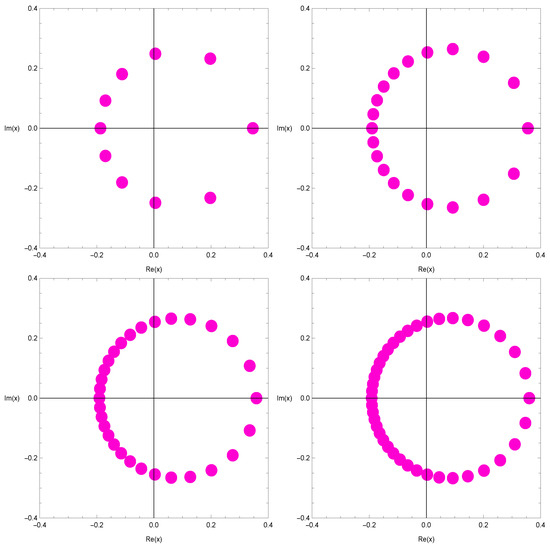
Figure 1. Zeros of $E_{n,p,q}^{\left(r\right)}\left(x\right)=0$.

In Figure 1 (top-left), we chose $r=7,n=10,p=1/2$ and $q=1/10$. In Figure 1 (top-right), we chose $r=7,n=20,p=1/2$ and $q=1/10$. In Figure 1 (bottom-left), we chose $r=7,n=30,p=1/2$ and $q=1/10$. In Figure 1 (bottom-right), we chose $r=7,n=40,p=1/2$ and $q=1/10$. We can see that distribution of zeroes of $E_{n,p,q}^{\left(r\right)}\left(x\right)=0$ is very regular. Therefore, the theoretical prediction of the regularity of distributions of the zeros of $E_{n,p,q}^{\left(r\right)}\left(x\right)=0$ will remain as future research problems (Table 1).

Now, we have the numerical solution satisfying higher-order Euler polynomials $E_{n,p,q}^{\left(r\right)}\left(x\right)=0$ for $x\in \mathbb{R}$. The numerical solutions of the higher-order Euler polynomials $E_{n,p,q}^{\left(r\right)}\left(x\right)=0$ are listed in Table 2 about a fixed $r=3,p=\frac{1}{2}$, and $q=\frac{1}{10}$ and different value of n.

The ∗ mark in Table 2 means that there is no solution of $E_{n,p,q}^{\left(r\right)}\left(x\right)=0$.

6. Conclusions and Future Developments

This paper introduced the Carlitz’s form higher-order Euler numbers and polynomials. We have induced some formulas about the Carlitz’s form Euler numbers and polynomials with high-order. Symmetric identities about Carlitz’s form Euler numbers and polynomials with high-order are also gained. In addition, the result of [19] is a special case of $r=1$, which can be induced from our paper. We make the following conjectures by numerical experiments:

Conjecture 1.

Prove or disprove that $E_{n,p,q}^{\left(r\right)}\left(x\right),x\in \mathbb{C},$ has $Im\left(x\right)=0$ reflection symmetry analytic complex functions. Furthermore, $E_{n,p,q}^{\left(r\right)}\left(x\right)$ has $Re\left(x\right)=a$ reflection symmetry for $a\in \mathbb{R}$.

It have been checked about many values of n. It is still unknown when the conjecture 1 is true or false about each value n (see Figure 1).

In Table 1, there is no solution of that the Carlitz’s form $(p,q)$-Euler polynomials with higher-order is 0. Find such n so that there is no solution. If the Carlitz’s form $(p,q)$-Euler polynomials with higher-order has solutions, it is doubtful whether it has distinct solutions.

Conjecture 2.

Prove or disprove that $E_{n,p,q}^{\left(r\right)}\left(x\right)=0$ has n distinct solutions.

We use the following symbols. $R_{E_{n,p,q}^{\left(r\right)}\left(x\right)}$ denotes the number of real zeros of $E_{n,p,q}^{\left(r\right)}\left(x\right)=0$ on the real plane $Im\left(x\right)=0$ and $C_{E_{n,p,q}^{\left(r\right)}\left(x\right)}$ denotes the number of complex zeros of $E_{n,p,q}^{\left(r\right)}\left(x\right)=0$. We can check $R_{E_{n,p,q}^{\left(r\right)}\left(x\right)}=n-C_{E_{n,p,q}^{\left(r\right)}\left(x\right)}$(see Table 1 and Table 2) because n is the degree of the polynomial $E_{n,p,q}^{\left(r\right)}\left(x\right)$.

Also, when the Carlitz’s form higher-order $(p,q)$-Euler polynomials is 0, if the equation has solutions, we have the following question:

Conjecture 3.

Prove or disprove that

$$R_{E_{n,p,q}^{\left(r\right)}\left(x\right)}=\left\{\begin{array}{cc}1,\hfill & \mathrm{if}n=\mathrm{odd},\hfill \\ 2,\hfill & \mathrm{if}n=\mathrm{even}.\hfill \end{array}\right.$$

We expect that the research in this direction will be a new approach using numerical methods for the study of Carlitz’s form Euler polynomials $E_{n,p,q}^{\left(r\right)}\left(x\right)=0$ (See [13,17,19,20]).

References

- Araci, S.; Duran, U.; Acikgoz, M.; Srivastava, H.M. A certain (p, q)-derivative operato rand associated divided differences. J. Ineq. Appl. 2016, 2016. [Google Scholar] [CrossRef]
- Andrews, G.E.; Askey, R.; Roy, R. Special Functions. In Encyclopedia of Mathematics and Its Applications 71; Cambridge University Press: Cambridge, UK, 1999. [Google Scholar]
- Carlitz, L. Expansion of q-Bernoulli numbers and polynomials. Duke Math. J. 1958, 25, 355–364. [Google Scholar] [CrossRef]
- Choi, J.; Srivastava, H.M. The Multiple Hurwitz Zeta Function and the Multiple Hurwitz-Euler Eta Function. Taiwan. J. Math. 2011, 15, 501–522. [Google Scholar] [CrossRef]
- Choi, J.; Anderson, P.J.; Srivastava, H.M. Carlitz’s q-Bernoulli and q-Euler numbers and polynomials and a class of generalized q-Hurwiz zeta functions. Appl. Math. Comput. 2009, 215, 1185–1208. [Google Scholar]
- Guariglia, E.; Silvestrov, S. A functional equation for the Riemann zeta fractional derivative. AIP Conf. Proc. 2017, 1798, 020063. [Google Scholar]
- Guariglia, E. Fractional derivative of the Riemann zeta function. In Fractional Dynamics; De Gruyter: Berlin, Germany, 2015; pp. 357–368. [Google Scholar]
- He, Y. Symmetric identities for Carlitz’s q-Bernoulli numbers and polynomials. Adv. Diff. Equ. 2013, 246, 10. [Google Scholar] [CrossRef]
- Kim, D.; Kim, T.; Seo, J.-J. Identities of symmetric for (h, q)-extension of higher-order Euler polynomials. Appl. Math. Sci. 2014, 8, 3799–3808. [Google Scholar]
- Kim, T. Barnes type multiple q-zeta function and q-Euler polynomials. J. Phys. A Math. Theor. 2010, 43, 255201. [Google Scholar] [CrossRef]
- Li, C.; Dao, X.; Guo, P. Fractional derivatives in complex planes. Nonlinear Anal. 2009, 71, 1857–1869. [Google Scholar] [CrossRef]
- Ortigueira, M.D. A coherent approach to non-integer order derivatives. Signal Process. 2006, 86, 2505–2515. [Google Scholar] [CrossRef]
- Ryoo, C.S. (p, q)-analogue of Euler zeta function. J. Appl. Math. Inform. 2017, 35, 113–120. [Google Scholar] [CrossRef]
- Simsek, Y. Twisted (h, q)-Bernoulli numbers and polynomials related to twisted (h, q)-zeta function and L-function. J. Math. Anal. Appl. 2006, 324, 790–804. [Google Scholar] [CrossRef]
- Srivastava, H.M. Some generalizations and basic (or q-) extensions of the Bernoulli, Euler and Genocchi Polynomials. Appl. Math. Inform. Sci. 2011, 5, 390–444. [Google Scholar]
- Kurt, V. A further symmetric relation on the analogue of the Apostol-Bernoulli and the analogue of the Apostol-Genocchi polynomials. Appl. Math. Sci. 2009, 3, 53–56. [Google Scholar]
- Agarwal, R.P.; Kang, J.Y.; Ryoo, C.S. Some properties of (p, q)-tangent polynomials. J. Comput. Anal. Appl. 2018, 24, 1439–1454. [Google Scholar]
- Duran, U.; Acikgoz, M.; Araci, S. On (p, q)-Bernoulli, (p, q)-Euler and (p, q)-Genocchi polynomials. J. Comput. Theor. Nanosci. 2016, 13, 7833–7846. [Google Scholar] [CrossRef]
- Ryoo, C.S. Some symmetric identities for (p, q)-Euler zeta function. J. Comput. Anal. Appl. 2019, 27, 361–366. [Google Scholar]
- Ryoo, C.S. On the generalized Barnes type multiple q-Euler polynomials twisted by ramified roots of unity. Proc. Jangjeon Math. Soc. 2010, 13, 255–263. [Google Scholar]
© 2019 by the authors. Licensee MDPI, Basel, Switzerland. This article is an open access article distributed under the terms and conditions of the Creative Commons Attribution (CC BY) license (http://creativecommons.org/licenses/by/4.0/).