1. Introduction
The Nambu-Jona-Lasinio (NJL) model represents one of the earliest attempts to describe the strong interactions between protons and neutrons inside an atomic nucleus. Even though today we know a better suited description of these interactions at the fundamental level, namely, among quarks, in the form of the gauge theory called Quantum Chromodynamics (QCD), the simplicity of the NJL model and its ability to gasp, at least to some extent, robust details of the strong interactions make it a favorite candidate to explore the dynamic of strongly interacting particles under extreme conditions. The NJL model describes Dirac fermions—quarks in modern considerations—that interact at contact in the form of a four-fermion interaction with a single coupling constant. One of the main features of the model, and the one we are interested in, is the phenomenon of spontaneous chiral symmetry breaking through an analogy to the BCS theory of superconductivity [
1,
2]. As an outcome of this symmetry breaking, the fundamental fermion fields acquire a mass that turns out to be a constant. Thus, to give this prediction a physically reliable character, it should be valid only up to some scale. In this sense, the model is non-renormalizable, and thus for the loop integrals to converge, the introduction of a regularization scheme is necessary. The model has been extended to provide it with more reliable features, close to those exhibited in QCD. It can be coupled to the Polyakov loop through an effective potential to describe confinement [
3]. It can also be regularized non-locally such that the quark mass function smoothly varies with energy [
4]. Other variants make the model suitable for the description of strong interactions in an effective and refined manner. For a review on the NJL model, we refer the readers to the seminal works in [
5,
6].
On the other hand, addition of a heat bath or density effects in the model is straightforward. These ingredients are the key to study the QCD phase diagram to understand the last transition that hadronic matter experienced during the early Universe as it expanded and cooled down. Moreover, the recent interest of incorporating the effect of an external magnetic field has been boosted by the fact that in heavy-ion collisions, very strong magnetic fields are generated in the interaction region, changing the behavior of the above transition [
7,
8]. Under these circumstances, the role of these external agents in the NJL model is translated into an effective enhancement or dilution of the strength of the coupling constant as compared with that of vacuum [
8,
9]. Therefore, it is worth exploring the parametric behavior of the solution to the gap equation of the model for arbitrarily large values of the coupling. This is the main subject of this article.
A favorite strategy to solve the gap equation is to cast it in a transcendental form and then use iterations to find the dynamical mass self-consistently [
10,
11]. Each iteration is then explained in terms of the number of self-energy insertions into the fermion propagator that are being re-summed non-perturbatively. The spirit of this approach is that starting with a given initial guess, after a finite number of iteration steps, one is arbitrarily close to the actual solution. This seemingly harmless procedure has in fact proven to be very robust for the hard cut-off regulators even for large values of the coupling constant. However, for other regulation schemes such as the Pauli-Villars and proper time, surprises appear from the behavior of this procedure, as was noticed by [
10,
11,
12] and we revise in deeper detail in this work. To this end, we have organized the remaining of the article as follows: In
Section 2 we review the basics of the model. In
Section 3 we present the parametric form of the gap equation for the different regularization schemes, whereas
Section 4 is devoted to describing the iterative procedure to find the solution of the gap equation in vacuum for different regularization schemes. We add the influence of a magnetized, thermal medium and explore once more the traits of the iterative solution in
Section 5. Conclusion and final remarks are presented in
Section 6.
2. NJL Model and the Gap Equation
The Lagrangian for the NJL model is
In modern considerations,
is regarded the quark field,
is the current quarks mass,
G is the coupling constant and
are the Pauli matrices acting on isospin space. In this Lagrangian, only scalar and pseudoscalar interactions are considered. To explicitly observe the spontaneous breaking of chiral symmetry in the model, we commence from the gap equation. Such an equation states important features of general Quantum Field Theories with spontaneous symmetry breaking, among which it highlights the fact that the ground state does not possess the same symmetry of the underlying Lagrangian. Breaking of the chiral symmetry of the model is due to an interaction which induces a pairing of particles and anti-particles (chiral condensate) resembling the Cooper pair structure of a Type-II Superconductor. Even from the early discussion of the model, within the Hartree-Fock approximation, the gap equation emerges as a constraint that minimizes the total energy of the system. In the local version of the model, it has the simple form
where
m is the dynamically generated mass and
is the so-called chiral condensate, defined as
with
the dressed quark propagator
One of the characteristics of the NJL model is that the predicted dynamically generated mass is independent of the momentum, making the model an effective description of low-energy QCD. As we mentioned before, the model is non-renormalizable, and thus a regularization scheme must be used for the integrals involved to converge. For the purposes of this work, we review some of the most commonly used schemes, namely, the
-cut-off (
), the
-cut-off (
), Pauli-Villars (PV) and proper time (PT) regularizations. Then, the gap equation in vacuum in each of these regularization schemes is written as
respectively. Here,
is the number of quark families,
is the number of colors considered and
is the incomplete gamma function defined as
To ease the analysis of the solutions to Equations (5)–(8), we express the above relation in dimensionless form,
where we introduce the dimensionless quantities
for all regularizations and
for 4D, PV, and PT, whereas
for the 3D regularization schemes. Below we introduce the method to solve the gap equations in Equations (10)–(13) using iterations.
3. Solving the Gap Equation with Iterations
To solve the gap equations described above, we introduce the notation
where
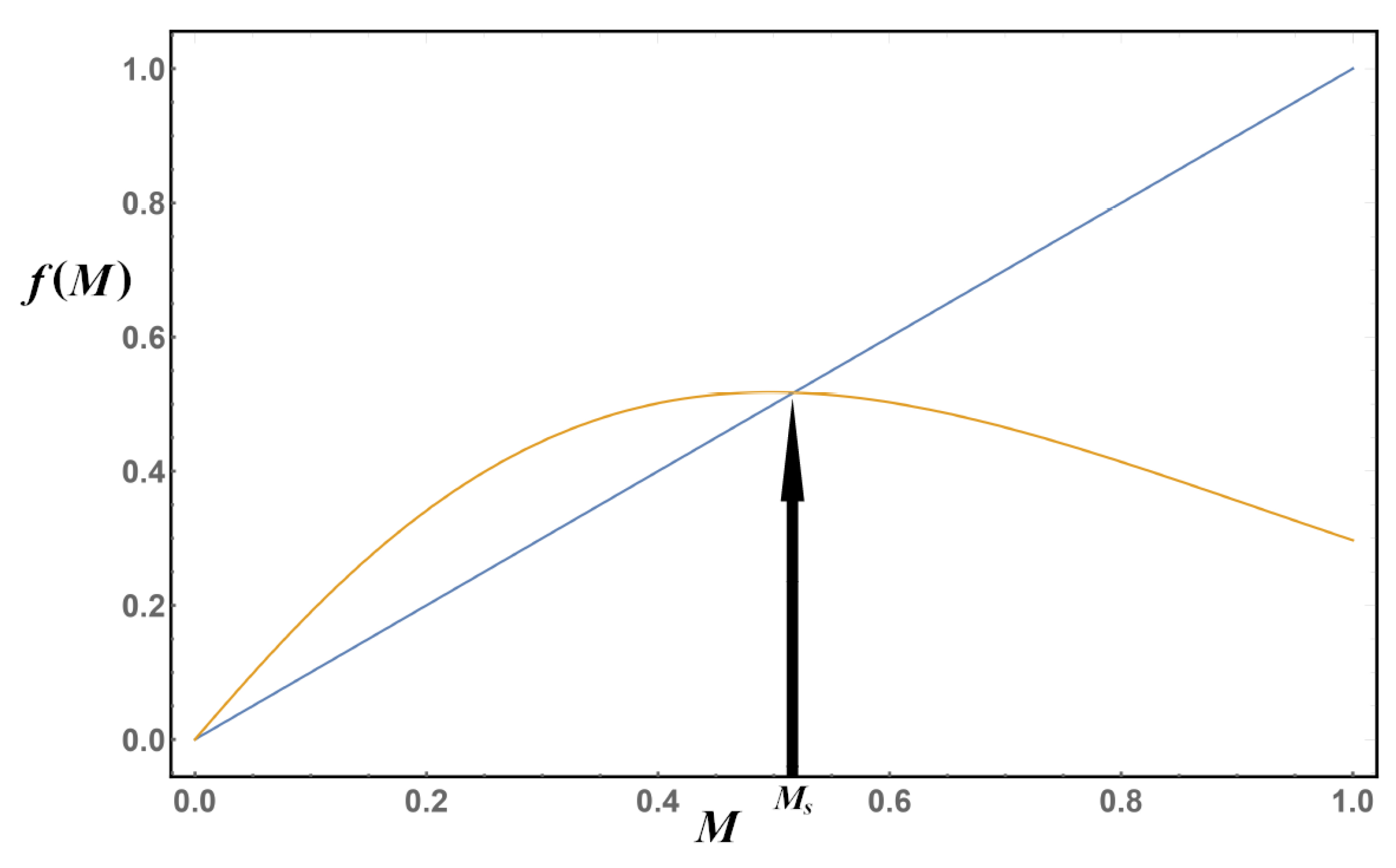
is the function on the right-hand-side (RHS) of any of the gap equations in Equations (10)–(13). If we plot the two equations
y and
as functions of
M for a fixed value of
, for example, we get
Figure 1.
As we can see from
Figure 1, the solution of the system of equations in Equation (
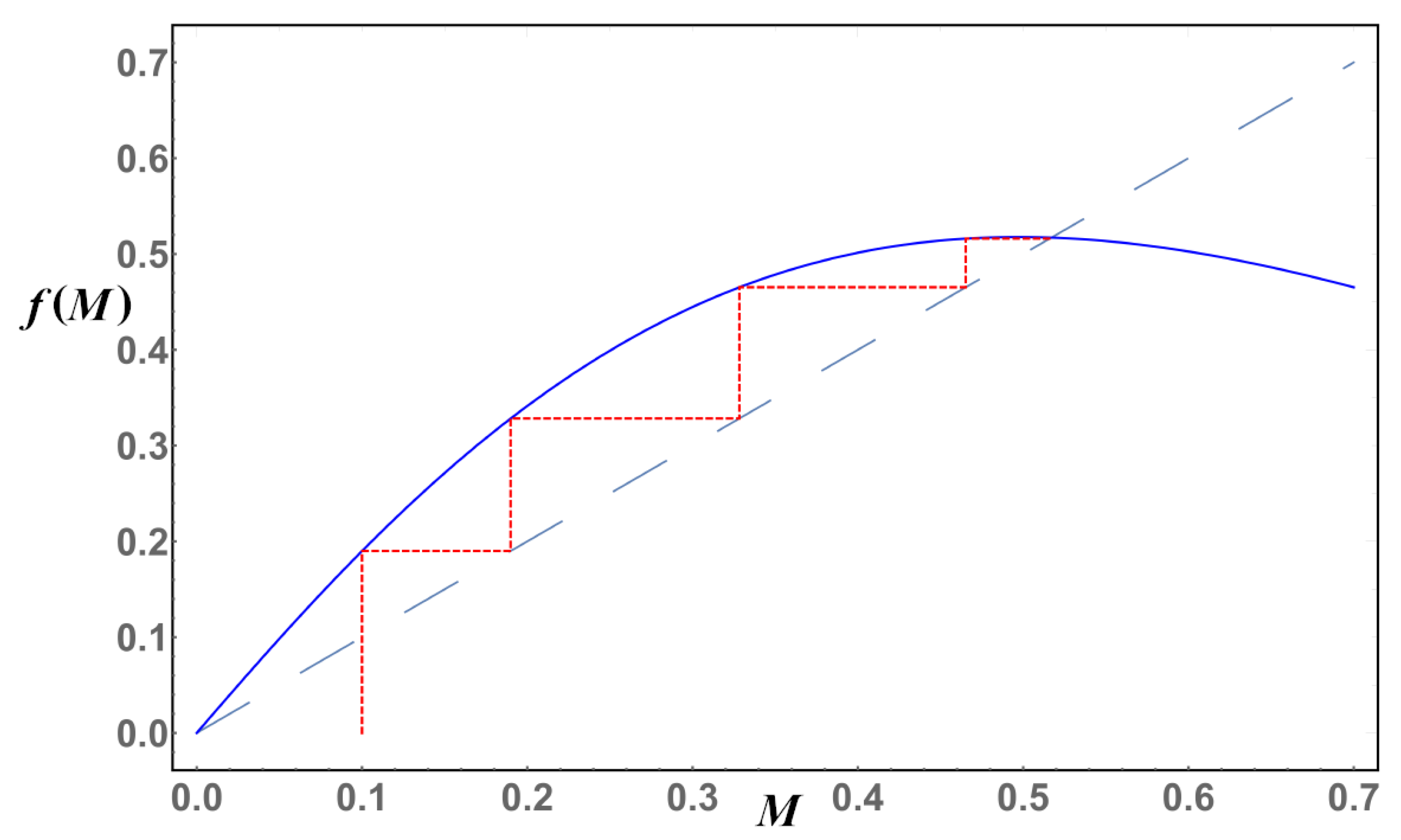
14) is the intersection of the two curves. Our goal is then to catch this solution using iterations. The iterating procedure can be depicted in a cobweb plot, a visual tool that depicts the iterative process by joining with straight lines the beginning (vertical) and end (horizontal) of each iteration,
Figure 2. For each value of the coupling constant, we can construct the corresponding cobweb plot. Our main interest is to locate the point where the iterations converge. By definition, this point corresponds to the solution of the gap equation for that particular value of
. We thus apply the following iteration procedure to the Equations (10)–(13):
We select a value of to start with,
We pick a positive initial random value of mass and plug it in the RHS of the gap equation,
For the selected value of the coupling, , we perform a sufficiently large number of iterations; we use 500 iterations,
We store and plot the last 70 iterations obtained; for a converging solution, all these 70 values should be on top of each other in the corresponding plot.
We then pick another value of and repeat.
In the next section we show the results obtained from this iteration procedure. We insist that this procedure corresponds to self-energy insertions into the fermion propagator in a non-perturbative re-summation [
10,
11].
4. Results: Gap Equation in Vacuum
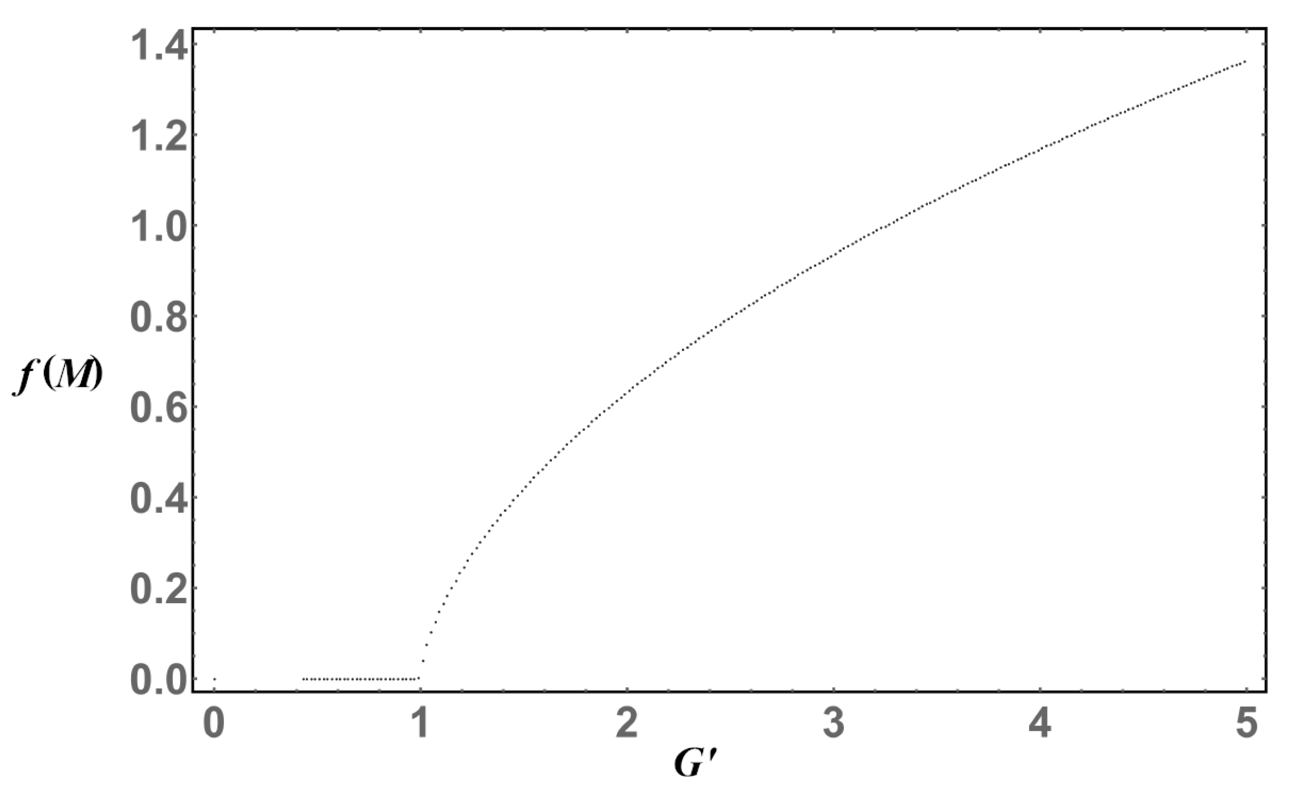
Now we proceed to analyze the results given by the iterative method described above. In
Figure 3, we plot the last 70 steps of the iteration procedure carried out for Equation (
10) for each value of the coupling
. As we can see, the plotted curve gives the characteristic behavior expected for a solution of the gap equation; for a range of values for the coupling, where it is not strong enough, the solution to the gap equation is just the trivial one
. Then, at the critical value of the coupling
, masses start to be dynamically generated. It should be noted nevertheless that because we are working with dimensionless quantities, the value of
changes for different regularization schemes. For example, in Equation (
5),
, provided we take
and
. Finally, we observe a monotonic growth of the dynamical mass as a function of the coupling
.
Next, for Equation (11), the iterative procedure is shown in
Figure 4. Just like in the previous case, there is a critical value for the coupling,
, to break the chiral symmetry. In this regularization scheme, we can see that the mass grows monotonically, but slowly as a function of the coupling constant in comparison with the
regularization scheme.
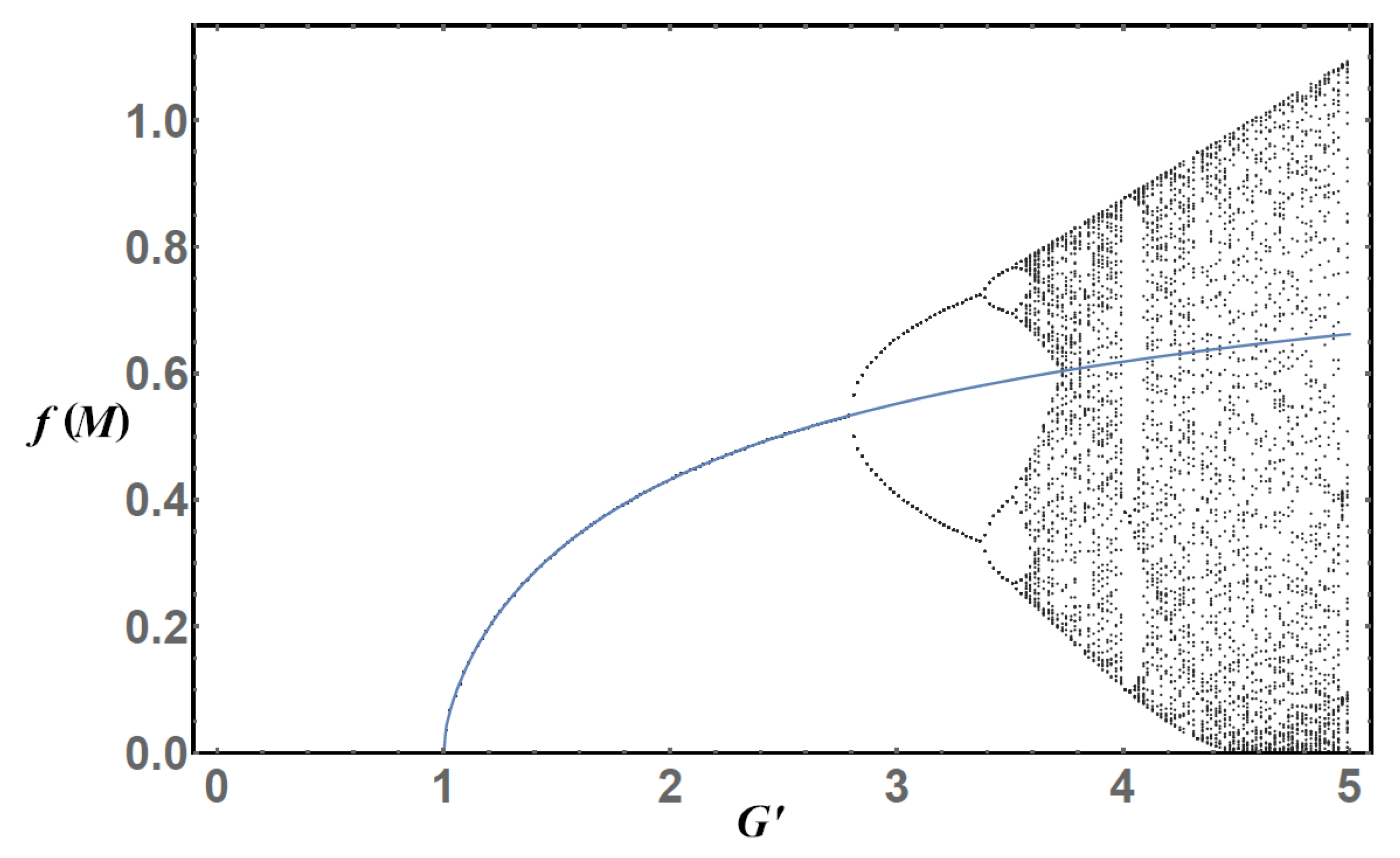
So far, the iterative procedure has converged as expected. This means the non-trivial and non-negative solution of the gap equation can be found through this procedure and is unique. The first example of the iterative procedure failing to converge is shown in
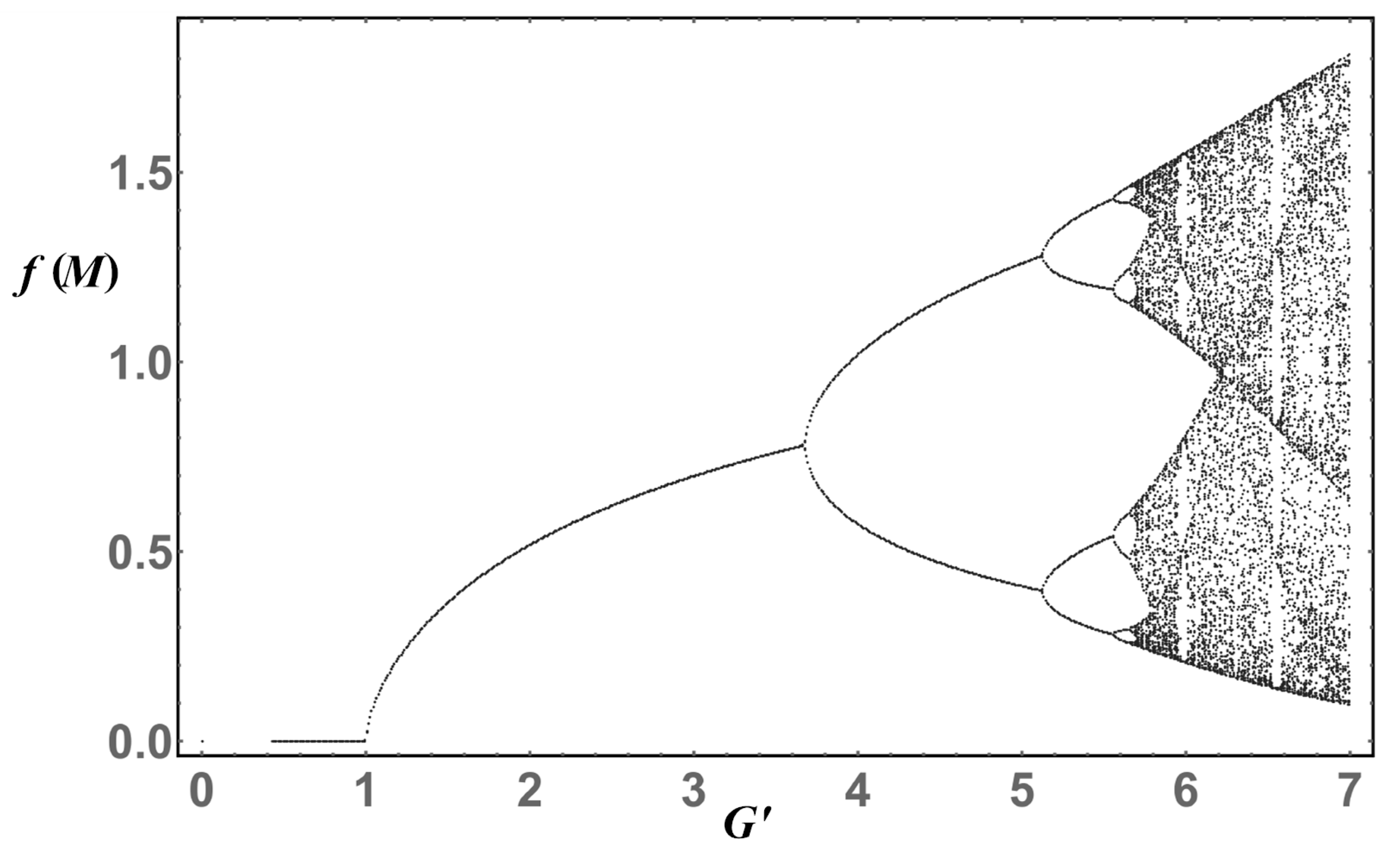
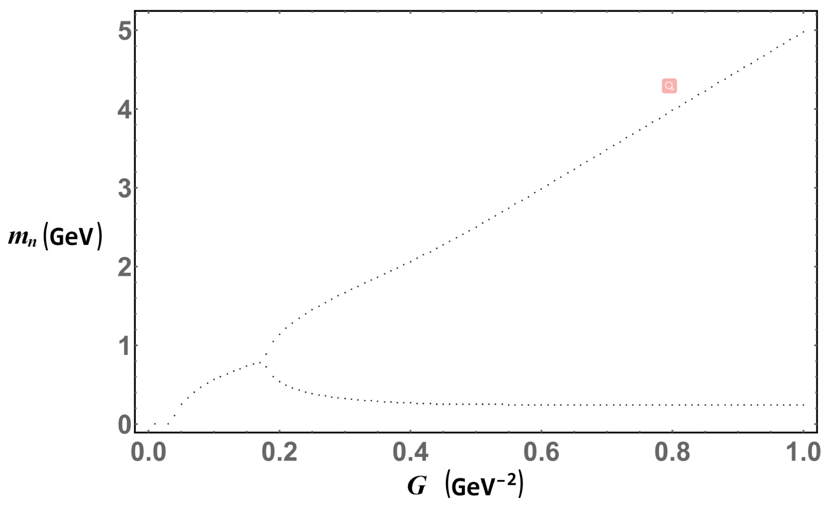
Figure 5, corresponding to Equation (12). The first feature that pops to the eye is the non-converging region of the
Figure 5, similar to the one found in the logistic map [
13]. Around
, a second bifurcation appears. The nature of this flip bifurcation implies that the iterative procedure is bouncing between two values. Moreover, when
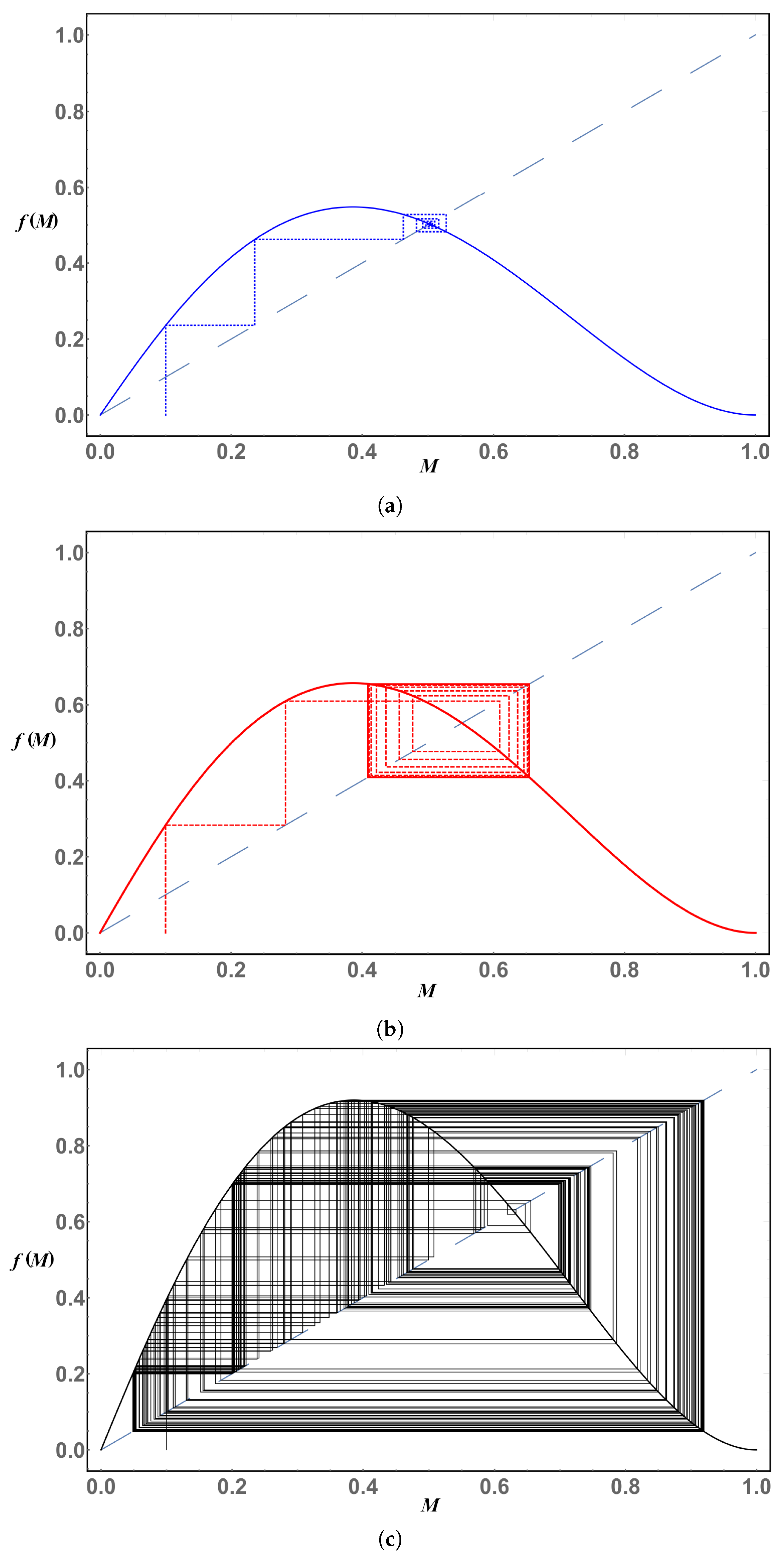
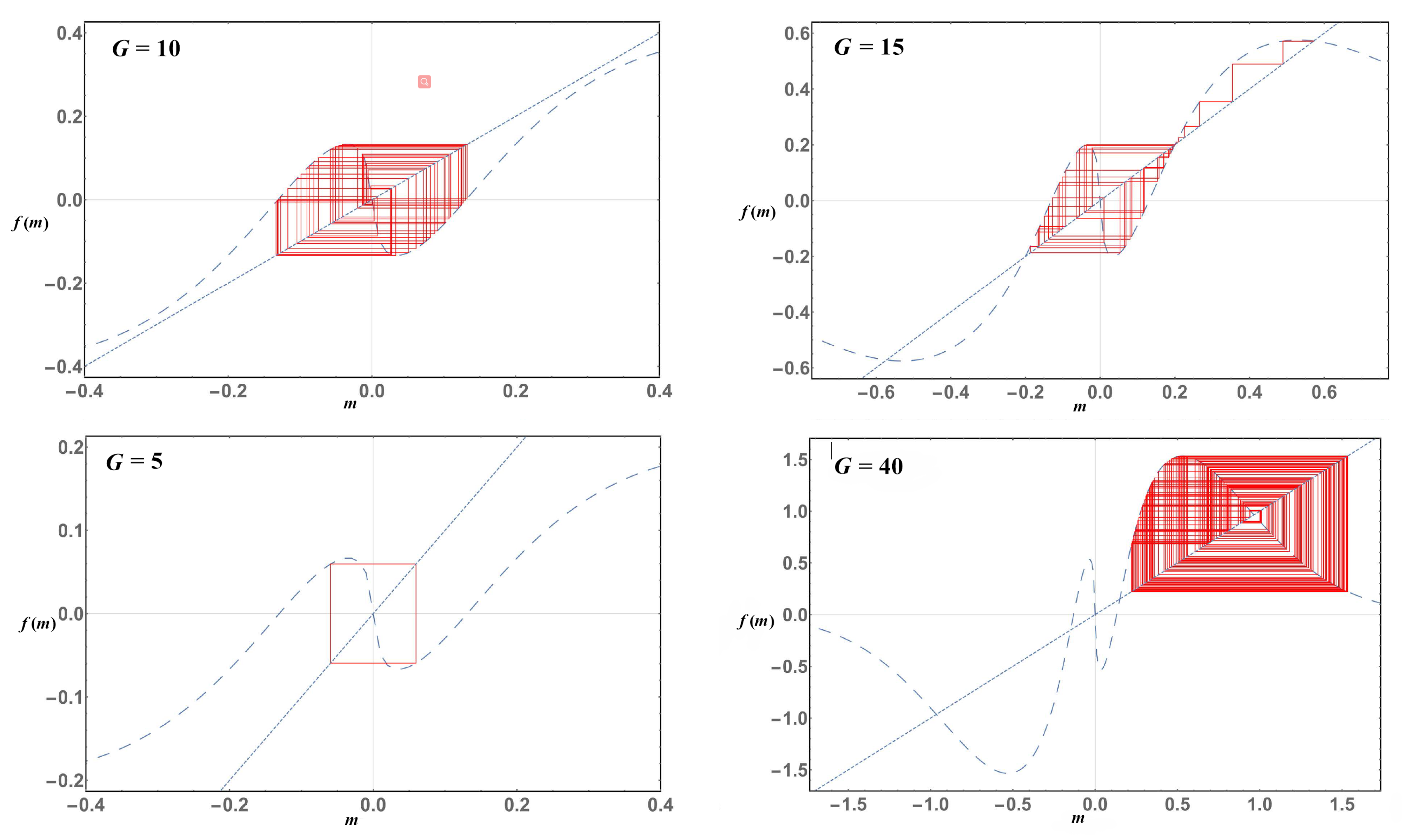
new bifurcations appear and so on as the coupling grows, until the iteration procedure becomes chaotic. This behavior is better seen in a cobweb plot, as shown in
Figure 6. We draw the cobweb plot of three particular values of the coupling constant: For
(top), the iteration procedure successfully converges and the solution to the gap equation is achieved; for
(middle), the iterative procedure ceases to converge and each iteration bounces between two values, orbiting around the solution of the gap equation; for
, we lose any pattern in the iterations and the procedure becomes chaotic.
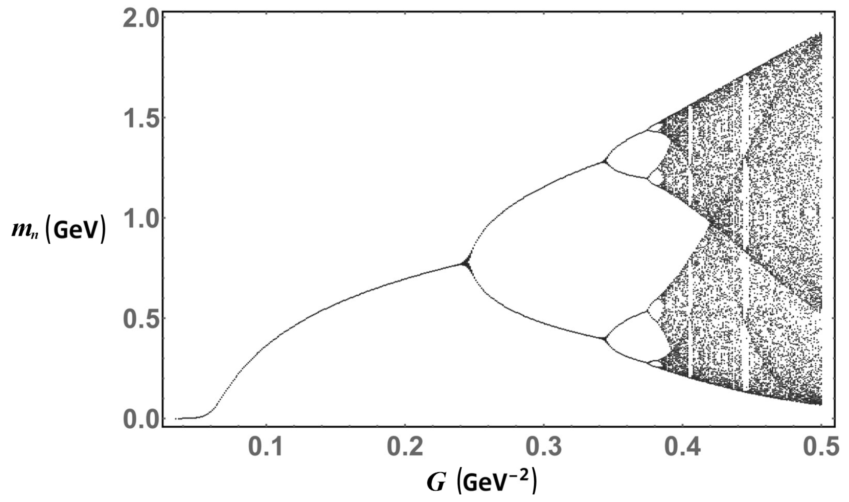
Finally, for the PT regularization scheme, Equation (13), the plot of iterations for different couplings can be seen in
Figure 7. In a similar fashion to the PV regularization scheme, firstly we have that only the trivial solution is found though this approach, followed by a behavior consistent with the expected solution for values of
, but upon increasing the coupling
, the iterative procedure ceases to converge and becomes chaotic. It is worth mentioning that the chaotic behavior of the PT regularization scheme has been found to hold even in higher dimensions [
14]. Additionally, it should be stressed that even though the iterative procedure does not converge after
the solution still can be found with others numerical methods, as shown in the same
Figure 5, were we plot the minimum solution of the gap equation Equation (12) and the iterative process. It should be remarked that the iterative method, if converges, is only capable of finding the solutions that behave as an attractor in the gap equation. This becomes important if the gap equation supports multiple positive solutions. An example of this is Equation (12) that has two positive solutions for each value of the coupling
. Fortunately, one advantage of solving the gap equation in an iterative manner is that the iterations tend to converge to the smallest of the two solutions, which behaves as an attractor and is the one that minimizes the thermodynamic potential, making it the physically meaningful.
As we have seen, the application of an iterative procedure to solve the gap equation in any regularization scheme may seem straightforward. Nevertheless, we have found that for two of the most popular regularization schemes, such a procedure fails to converge, albeit for the physically relevant region of coupling constant describing the pion phenomenology in vacuum, the iterations converge smoothly. While it is true that the values of the coupling must be very high for the iterative procedure to fail, it is well known that external factors such as magnetic fields, through the phenomenon of magnetic catalysis, enhance the formation of the chiral condensate in such a way that the effect of the coupling constant on the gap equation magnifies, thus leaving the possibility that even for small values of the coupling, the iterative procedure cease to converge. In other regularization schemes, adding the effects of an external magnetic fields is not as straightforward as with the PT regularization, where we adopt the Schwinger representation of the propagator [
15] and use the proper time regularization scheme to get the gap equation in an external magnetic field. Another widely application of the NJL model is the inclusion of the temperature using the Matsubara formalism [
16], and contrary to an external magnetic field, the thermal bath dilutes the chiral condensate. Therefore, it is worth exploring the behavior of the iteration procedure in a medium, as we do below.
5. Gap Equation in A Medium
As we mentioned before, for its simplicity, the NJL model can be easily extended to account for medium effects as magnetic fields and a thermal bath. The effects of an external magnetic field can be introduced in the model using the Schwinger representation of the fermion propagator, which has the form
where
is the absolute value of the quark charge,
and
for the up and down quarks, respectively,
B is the magnetic field strength and we have chosen the homogeneous magnetic field to point in the
direction such that
and
are defined as
Substituting Equation (
15) into Equation (
3) and taking the trace, we get the chiral condensate in a homogeneous magnetic field to be given by
where we are using the simplified notation
. To proceed further, we first perform the integration on the perpendicular component of momentum and upon performing a Wick rotation
, we get,
Our next goal is to add the effects of temperature. We do so within the Matsubara formalism, through the substitutions
where
are the Matsubara frequencies. To get the final form of the condensate, we carry out the remaining momentum integrals and perform a change of variable
, namely,
With the condensate in Equation (
20) we can get the gap equation and, in principle, calculate the dynamical mass. Nevertheless, we would like to explicitly separate the contribution of vacuum, which needs regularization. We can identify the sum inside Equation (
20) with the Jacobi theta function
and
. Thus,
where we have used the inversion formula [
17].
Replacing Equation (
22) into Equation (
20), we get the expression for the chiral condensate that includes the thermomagnetic effects of the medium
Finally, the gap equation becomes
Then, to isolate the vacuum contribution to the gap equation, we split the first term of the theta function from the definition
and adding and subtracting a factor
in Equation (
25), we are led to
It should be noted that the integrals in Equation (
27) that involve the magnetic field or the temperature do not require to be regularized. This is so because the divergences in the NJL model appear only in the vacuum term, whereas the medium integrals converge without issues. Then, Equation (
27) is the expression we were looking for. If we take the limits
and
, we return to the gap equation in vacuum Equation (8), as expected. Moreover, from Equation (27), we may get the respective gap equations for the magnetic case (
), Equation (
28), or the thermal case (
), Equation (
29),
From here, our next goal is to set up the iteration procedure developed in the previous section to the gap equations Equations (
27)–(
29), but unlike the vacuum case, here we use dimensionful quantities. For the sake of clarity, although we got the gap equation containing both magnetic and thermal contributions, Equation (
27), we discuss each component separately. Fixing the regularization parameter
and performing the iteration procedure of the above section to Equation (
28), we obtain
Figure 8, with fixed
. As we can see, the behavior of the iterations for different values of the coupling is pretty much the same as that of the gap equation in vacuum, Equation (13). Nevertheless, there are a few remarkable differences. First and foremost, unlike the vacuum case, it does not exist a
hard critical value of the coupling constant
G from where the dynamical mass starts being generated. In other words, the derivative of the mass function
obtained is continuous for
and up to the first bifurcation. This can be seen because the transition between a zero value of dynamical mass and a non-zero value of mass is smooth, as a direct consequence of the magnetic field by the magnetic catalysis phenomenon: at a fixed
B, masses are generated at any weak value of the coupling constant. In fact, this smoothness is responsible for the non-existence of a critical coupling
[
18].
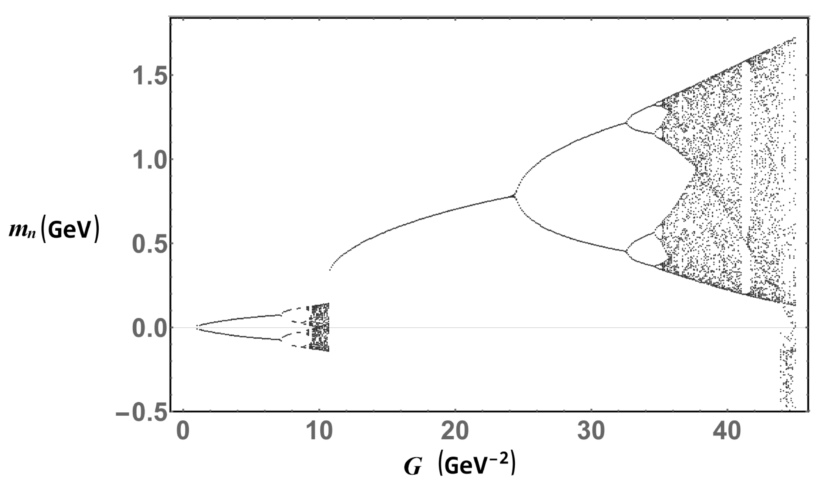
Coming up next, in
Figure 9 we show the iterations performed with Equation (
29) for
. Now the picture changes dramatically. At first glance, the general structure is similar to the free and magnetic cases, but at a closer inspection we find from the beginning and up to
that the iterations do not converge and, in fact, they bounce taking positive and negatives values. Furthermore, as the coupling approaches
, it appears what looks like a small version of the chaos found before,
Figure 7 and
Figure 8. This can be understood if we take a look at
Figure 10, where we show the cobweb plot for
,
,
and
. On the other side of the spectrum, we confirm the effect of the thermal bath on the condensate, the delay in the breaking of the chiral symmetry, for the iterations to converge the coupling strength must be in the order of
. This is 100 times more than in the magnetic case and around 60 times more than in the vacuum case. One can notice too that the starting point of the first bifurcation, and all the second chaos region in fact, has been delayed due the introduction of the temperature into the system.
Finally,
Figure 11 shows the last 70 iterations for
and
. The change is dramatic from the former case. First, the chaotic region is gone, and the only remainder is the sole bifurcation that occurs at
. One may be tempted to interpret this bifurcation as two different solutions, but this behavior is solely an effect of the non-convergence of the bifurcations. Another feature is that unlike the magnetic case, the hard breaking of chiral symmetry is present at
. Physically in the sole magnetic case,
B enhances the formation of the chiral condensate making the symmetry breaking
soft, where for any value of the coupling, mass is generated, though very small in magnitude. On the other hand, the thermal bath tries to dilute the condensate. In consequence, there appears a gap in the mass spectrum. Put together, the thermal bath forces the apparition of a
hard critical coupling at
, meanwhile the magnetic field enhances the chiral condensate. Thus, the coupling necessary for breaking the chiral symmetry goes down dramatically.
6. Conclusions and Final Remarks
In this article, we have revisited the commonly used iteration procedure to self-consistently solve the gap equation in the NJL model. Besides the coupling constant, the model has as a dynamical parameter a regulator that gives physical reliability to its predictions, namely, by choosing appropriately the coupling and regularization scale, one is able to predict static the properties of pions, for example. Such a regulator can be implemented through several prescriptions. Performing hard cut-offs on the three-momentum or directly on the four momentum, one observes the need for the coupling to reach a critical value before it is strong enough as to break chiral symmetry. By increasing the coupling constant further, the solution to the gap equation is always found for a sufficiently large number of iterations.
However, this procedure fails in other regularization schemes such as PV and PT. Though the iteration is stable and converges for small values of the coupling and up to the physically relevant values of this parameter, as it increases to a superstrong regime, the iteration procedure ceases to be stable such that at a second critical point, the iterations bounce between two values separated apart from the actual solution to the gap equation. Increasing further doubles the period and so on until a chaotic behavior unexpectedly emerges. We stress that this behavior indicates the failure of the iteration procedure, not that the gap equation develops new solutions.
Adding the influence of an external magnetic field alone, although similar in shape to that of vacuum, the magnetic catalysis phenomenon taking place in the model makes chiral symmetry to be broken at any weak coupling value. On the other hand, in a thermal bath at temperature T, the iterations make an unexpected behavior bouncing between positive and negative values. Though the behavior collapses to a stable solution at intermediate values, again, increasing the coupling constant, a chaotic domain in the iterations develop. When the two ingredients are considered at the same time, the chaotic behavior is no longer developed by the iterations in the large coupling regime, though the procedure bounces between two values.
Overall, within this iterative procedure, we observe reasons to take with special care the iteration procedure to obtain the solution to the gap equation in the NJL model at large values of the coupling.
