Novel m—Polar Fuzzy Linguistic ELECTRE-I Method for Group Decision-Making

Abstract

Linguistic variables play a vital role in several qualitative decision environments, in which decision-makers assume several feasible linguistic values or criteria instead of a single term for an alternative or variable. The motivation for the use of words or sentences instead of numbers is that linguistic classification and characterizations are generally less precise than numerical ones. In this research article, we encourage the fuzzy linguistic approach and introduce the novel concept known as m-polar fuzzy linguistic variable (mFLV) to increase the affluence of linguistic variables based on m-polar fuzzy (mF) approach. An mF set is an effective concept for interpreting uncertainty and fuzziness. The concept of mFLV is more versatile and sensible for dealing with real-life problems, when data comes from qualitative and multipolar information. We also introduce an mF linguistic ELECTRE-I approach to solve multiple-criteria decision-making (MCDM) and multiple-criteria group decision-making (MCGDM) problems, where the evaluation of the alternatives under suitable linguistic values are determined by the decision-makers. Furthermore, we validate the efficiency of our proposed technique by applying it to real-life examples, such as the salary analysis of companies and by selecting a corrupt country. Finally, we develop an algorithm of our proposed approach, present its flow chart, and generate computer programming code.

1. Introduction

Problems related to uncertain situations generally exist in multiple-criteria decision-making (MCDM) and multiple-criteria group decision-making (MCGDM), which are precisely appealing because of the difficult state of affairs of modeling and uncertainties. Several theories have been developed to overcome MCDM problems such as probability; however, in several directions, uncertainty is not probabilistic in description but relatively vague or imprecise. Thus, other theories, such as fuzzy set theory and fuzzy logic [1,2] have been prosperously applied to handle immature, imprecise, and vague information. Usually, to hold such a vagueness and imprecision, where two or more fundamentals of imprecision occur simultaneously, the modeling tools of ordinary fuzzy sets are limited. To overcome these limited approaches, several extensions and generalizations of fuzzy sets have been introduced, including hesitant fuzzy sets (HFSs) [3], bipolar fuzzy sets (BFSs) [4] and m-polar fuzzy sets (mF sets) [5].

In 2014, mF set theory was introduced by Chen et al. [5], which is the generalization of bipolar fuzzy sets. An mF set on a set X is a mapping $\mu :X\to {[0,1]}^m$. The concept behind it is that the multipolar information occurs because data of real-world problems are sometimes from multiple characters and agents. The membership value in mF sets is more understanding in obtaining uncertainty of data. The mF sets concede higher graphical representation of vague data, which promotes significantly better investigation in similarity measures, incompleteness and data relationships. Akram [6] introduced several notions based on mF sets and mF graphs including certain metrics in m-polar fuzzy graphs, certain types of irregular m-polar fuzzy graphs, and m-polar fuzzy hypergraphs.

The preceding fuzzy tools are suitable for problems that are defined only in quantitative situations, but generally, uncertainty is due to vagueness in a sense that is adopted by decision-makers in problems whose description is relatively qualitative. For such a situation, the fuzzy linguistic approach introduced by Zadeh [7,8,9] provided favorable outputs in many areas and applications [10]. In abandoning accuracy in the face of intense complexity, it is common to analyze the purpose of what might be called linguistic variables, i.e., a variable whose values are not numbers but words or sentences in artificial or natural language. The motivation for the use of words or sentences instead of numbers is that the linguistic classification and characterizations are generally less precise than numerical ones and have interesting uses in group decision analysis [11,12,13,14,15]. The linguistic approach is very significant in the context of personalized individual semantics in CWW [16,17]. Liu and Su [18] introduced the extended TOPSIS based on trapezoid fuzzy linguistic variables. Selvachandran and Salleh [19] proposed the concept of intuitionistic fuzzy linguistic variables and intuitionistic fuzzy hedges.

In the review of the fuzzy linguistic approach, including the distinct linguistic generalizations and extensions, it is shown that the design of linguistic information has actually been limited up till now, because mainly it is based on the concentration of very simple and single terms that should encircle and direct the information arranged by the decision-makers, respecting a linguistic variable. In recent years, several researchers, including Liao et al. [20] discussed the distance and similarity measures for hesitant fuzzy linguistic term sets and their application in MCDM. Later, Riera et al. [21] introduced some interesting properties of the fuzzy linguistic model based on discrete fuzzy numbers to manage hesitant fuzzy linguistic information. A term set is constituted by the completeness of values of a linguistic variable, which in assumption could have an infinite number of elements. Nonetheless, in distinct settings and directions, decision-makers who have suggestions regarding the problems defined under uncertainty cannot efficiently suggest a single term as an interpretation of their ability; they are determining the several terms at the same time or looking for a more complex linguistic term that is not usually defined in the linguistic term set. Therefore, Rodrguez et al. [22] worked with a view to overcome such limitations, taking into account the idea under the concept of HFS, to deal with several values in a membership function in a quantitative setting.

Elimination and choice translating reality (ELECTRE) is one of the MCDM methods, used in situations in which the decision-maker wants to include different criteria, and there may be a robust collection associated with the nature of evaluation surrounded by several standards. The ELECTRE approach was first introduced by Benayoun et al. [23]. Govindan et al. [24] studied the ELECTRE and made a comprehensive literature review on methodologies and applications. They focused on papers dealing with applications or developments of ELECTRE and ELECTRE-based methods. The modified concept of ELECTRE known as ELECTRE-I was introduced by Roy [25]. Furthermore, this approach was expended in a variety of alternative variants. For the multiple attribute decision-making methods, applications and widely used versions of ELECTRE-I, readers are referred to [26]. In the literature, most of these methods have been combined with fuzzy set theory by many researchers. Sevkli [27] compared crisp and fuzzy ELECTRE methods for supplier selection problems. For the selection of academic staff, Rouyendegh and Erkan [28] used the concept of fuzzy ELECTRE. Vahdani et al. [29] presented the comparison of fuzzy ELECTRE method with intuitionistic fuzzy ELECTRE method. Hatami-Marbini et al. [30] applied the method of fuzzy group ELECTRE for the interpretation of haphazard waste reprocessing of plants. Devi and Yadav [31] proposed intuitionistic fuzzy ELECTRE to choose the proper location of plants under group decision-making environments. Zandi and Roghanian [32] introduced a novel fuzzy ELECTRE method based on VIKOR method. Kheirkhah and Dehghani [33] applied the fuzzy group ELECTRE method to the evaluation of quality of public transportation facilities. Vahdani and Hadipour [34] presented the technique of interval-valued fuzzy ELECTRE. Hatami-Marbini and Tavana [35] expanded the method of ELECTRE-I and introduced the method of fuzzy ELECTRE-I with numerical examples to illustrate the effectiveness of their proposed method. Asghari et al. [36] used fuzzy ELECTRE-I method for the analysis of mobile payment models. Furthermore, fuzzy ELECTRE-I technique was applied in evaluating catering firm alternatives by Aytac et al. [37] and an environmental effect evaluation method based on fuzzy ELECTRE-I was composed by Kaya and Kahraman [38]. For handling MCDM problems Wu and Chen [39] developed the concept of intuitionistic fuzzy ELECTRE-I method. Chen and Xu [40] proposed a novel MCDM technique by combining HFSs with ELECTRE-II method. Lupo [41] calculated the service quality of three international airports using ELECTRE-III approach. ELECTRE methods have played a very significant role in the group of outranking methods. These methods enable us to use incomplete knowledge. For other notations, decision-making techniques and applications, readers are referred to [42,43,44,45,46,47,48,49,50,51,52,53].

Decision-making [54] can be examined as a conclusion of some intellectual and psychological processes that lead to the selection of an alternative among several options. Typical decision-making problems are described as selecting a place to visit, deciding which candidate is suitable for election, or choosing the best car to buy. It is worth noting that decision-making is a distinctive human ability, which is not naturally guided and based on obvious or absolute assumptions. It does not demand specific and complete analysis of information about the set of feasible alternatives. This fact motivated several researchers to apply fuzzy set theory to discuss vagueness and uncertainty in decision processes [55,56]. In recent years, many researchers have proposed very interesting methodologies [57,58] applied MCDM evaluations such as Antucheviciene et al. [59] to solve civil engineering problems by means of fuzzy and stochastic MCDM methods, which promoted complex decision support systems to help decision-makers reach a solution.

All previously proposed methods are unable to deal with the situation where given data is in the form of sentences and words with m different numeric and fuzzy values with its crisp domain. To handle this kind of information, we introduce the novel concept of the m-polar fuzzy linguistic variable (mFLV) and develop the MCDM method for decision-making problems, because all the traditional methods are ineffectual for studying this type of imprecise behavior of linguistic computations and assessments. We apply the theory of mFLV to ELECTRE-I method to introduce the mF linguistic ELECTRE-I technique for MCDM and MCGDM. The proposed technique is useful, when given data is in the form of sentences and words with m different numeric and fuzzy values within its crisp domain. Unlike classical ELECTRE techniques, precise information is not used in analysis of alternatives and criteria. An mF linguistic ELECTRE-I approach is used to get more accurate and consistent results when we must eliminate the choices and to deal with the systems with more than one agreement. The proposed approach is more flexible as compared to various other extensions of ELECTRE-I, because in this method a variable and its linguistic values are considered to be fixed criteria for the ranking and evaluation of alternatives. All linguistic values are further classified by m different numeric and fuzzy values, which provide more accurate and compatible results as compared to other extensions of ELECTRE-I. This approach is valid for resolving decision-making problems in our daily life. The organization of this research article is as follows.

In Section 2, we review some basic concepts and propose the concept of an mFLV with its practical example. In Section 3, we present an mF linguistic ELECTRE-I approach for MCDM. In Section 4, we present an mF linguistic ELECTRE-I approach for MCGDM. We applied our mF linguistic ELECTRE-I approaches to real-life examples. We also present our proposed methods as an algorithm and generate computer programming code. In Section 6, we present a conclusion.

2. $\mathit{m}$—Polar Fuzzy Linguistic Variable

In this section, we review some basic concepts and propose the concept of an mFLV with its practical example.

Definition 1

([5]). An mF set on a universe X is a function $R=(p_1\circ R(r),p_2\circ R(r),\cdots ,p_m\circ R(r)):X\to {[0,1]}^m,$ where the i-th projection mapping is defined as $p_i\circ R:{[0,1]}^m\to [0,1].$ $\mathbf{0}=(0,0,\cdots ,0)$ is the smallest element in ${[0,1]}^m$ and $\mathbf{1}=(1,1,\cdots ,1)$ is the largest element in ${[0,1]}^m.$

Definition 2

([7]). Linguistic variables are variables whose values are words or sentences in a natural or artificial language. If these words are described by fuzzy sets that are defined over a universal set, then the variables are called fuzzy linguistic variables.

Definition 3

([7,12]). A linguistic term set is defined by means of an ordered structure providing the term set that is distributed on a scale at which a total order has been defined. For example, a set S of seven terms could be written as follows:

$$S=\{s_o=nothing,s_1=verylow,s_2=low,s_3=medium,s_4=high,s_5=veryhigh,s_6=perfect\}.$$

An m-polar fuzzy linguistic variable is a variable that considers words in natural language(s) as its values. The values of such a variable are characterized by mF sets that are defined in a universe that contains the variable.

Definition 4.

An m-polar fuzzy linguistic variable (mFLV) is characterized by a $4-$tuple $(L_v,V,P_d,M)$ such that

• $L_v$ is the name of an mFLV,
• V is the set of linguistic values of $L_v$,
• $P_d=[0,\infty ]$ is the physical domain in which an mFLV takes its crisp values,
• M is the semantic rule that relates every linguistic value in V to mF set.

We call the linguistic variable an mFLV, because its linguistic values are further classified by m different characteristics. However, $P_d$ is the physical domain in which an mFLV takes its crisp values and this domain can be arranged in parts for linguistic values according to given requirements. Finally, semantic rule M is described, which is actually a rule that differs the mFLV from previously defined linguistic variables. This rule relates the linguistic values $(V_l^{\prime }s|l=1,2,\cdots ,k)$ of mFLV with mF set, which shows that when each linguistic value is further classified by m different characteristics, the degree of linguistic values is defined by

$$d_l^i=p_i\circ d_l(V_l)\in [0,1],\mathrm{where}i=1,2,\cdots ,m.$$

It clearly shows m different characterizations of each linguistic value. The contribution of mFLV in real life is shown in Example 1.

Example 1.

Let “temperature" be a linguistic variable and $V=\{Hot,Warm,Cool,Cold\}$ be the set of its linguistic values. The physical domain for linguistic variable is $P_d=$ [0 ${}^{\circ }$C, 50 ${}^{\circ }$C], which is the set of real non-negative numbers, and each linguistic value has different range of physical domain given as follows

• For cold temperature, physical domain is 0 ${}^{\circ }$C to 10 ${}^{\circ }$C,
• For cool temperature, physical domain is 10 ${}^{\circ }$C to 20 ${}^{\circ }$C,
• For warm temperature, physical domain is 20 ${}^{\circ }$C to 30 ${}^{\circ }$C,
• For hot temperature, physical domain is 30 ${}^{\circ }$C to 50 ${}^{\circ }$C.

We call this linguistic variable a $3-$polar fuzzy linguistic variable (3FLV), because we describe a semantic rule M that relates each linguistic value in set V with a $3-$polar fuzzy set (3F set). According to the 3F set, each linguistic value is characterized as

• $p_1\circ d_l(V_l)$ serves as “heat energy”,
• $p_2\circ d_l(V_l)$ serves as “air pressure",
• $p_3\circ d_l(V_l)$ serves as “water vapors",

where $l=1,2,3.$ Thus, we have

$$\begin{array}{cc}\hfill L_v=\{& \langle Hot,(0.90,0.71,0.20)\rangle ,\langle Warm,(0.79,0.61,0.29)\rangle ,\hfill \\ & \langle Cool,(0.45,0.39,0.69)\rangle ,\langle Cold,(0.12,0.19,0.89)\rangle \}.\hfill \end{array}$$

In terms of the variable (temperature), four different linguistic values are discussed in Example 1, and each linguistic value is further classified by three different criteria or properties on which linguistic value shows its dependence. It shows the 3F restrictions on the values of a base variable. These 3F restrictions clearly show that each linguistic value totally depends on heat energy, air pressure, and water vapors. Thus, we call temperature a 3F linguistic variable by Definition 4.

3. $\mathit{m}$F Linguistic ELECTRE-I Approach for MCDM

In this section, we introduce an mF linguistic ELECTRE-I approach for MCDM problems, which is based on the concept of mFLV. We also apply this approach to real-life examples in Section 3.1, to show its importance and feasibility. In this approach, we choose $L_v$ an mFLV and $A=\{a_1,a_2,\cdots ,a_n\}$ the set of mFLV of different alternatives. According to this mFLV, we take $\left\{V_l\right|l=1,2,\cdots ,k\}$ the set of linguistic values. These linguistic values are classified by m different characteristics. The degree of each alternative ($a_p\in A,p=1,2,\cdots ,n$) over all the linguistic values $V_l^{\prime }s$ is given by mF set ${\wp }_p=\{(a_p,d_{pl}^i)|i=1,2,\cdots m\},$ where $d_{pl}^i=p_i\circ d_{pl}(a_p,V_l)\in [0,1]$ and $d_{pl}^i$ classify the different characteristics or properties of linguistic values. $P_d$ is the actual physical domain in which the mFLV takes its quantitative (crisp) values, i.e., $P_d=[0,+\infty ].$ In this case, we take the most suitable m values from the physical domain of each linguistic value. A decision-maker is responsible for evaluating mFLV of n different alternatives under k different linguistic values.

(i). Suitable ratings of alternatives are assessed in terms of m different characteristics under the physical domain $P_d$. Tabular representation of an mF linguistic decision matrix is given by

Table 1. Tabular representation of mF linguistic decision matrix.

$\mathit{m}-$Polar Fuzzy	Physical Domain
Linguistic	${\mathit{P}}_{{\mathit{d}}_1}$	${\mathit{P}}_{{\mathit{d}}_2}$	⋯	${\mathit{P}}_{{\mathit{d}}_{\mathit{k}}}$
Variable	$\mathit{m}-$Polar Fuzzy Linguistic Values
${\mathit{L}}_{\mathit{v}}$	${\mathit{V}}_{\mathbf{1}}$	${\mathit{V}}_{\mathbf{2}}$	⋯	${\mathit{V}}_{\mathit{k}}$
$a_1$	$(d_{11}^1,d_{11}^2,\cdots ,d_{11}^m)$	$(d_{12}^1,d_{12}^2,\cdots ,d_{12}^m)$	⋯	$(d_{1k}^1,d_{1k}^2,\cdots ,d_{1k}^m)$
$a_2$	$(d_{21}^1,d_{21}^2,\cdots ,d_{21}^m)$	$(d_{22}^1,d_{22}^2,\cdots ,d_{22}^m)$	⋯	$(d_{2k}^1,d_{2k}^2,\cdots ,d_{2k}^m)$
⋮	⋮	⋮	⋮	⋮
$a_n$	$(d_{n1}^1,d_{n1}^2,\cdots ,d_{n1}^m)$	$(d_{n2}^1,d_{n2}^2,\cdots ,d_{n2}^m)$	⋯	$(d_{nk}^1,d_{nk}^2,\cdots ,d_{nk}^m)$

.

(ii). Decision-maker has an authority to assign weights to each linguistic value of mFLV of alternatives according to his choice and the importance of each linguistic value. We discuss the case of mFLV so the decision-maker must assign the weights in terms of linguistic term set $L=\{{\mathrm{L}}_1=\mathrm{very}\mathrm{low},{\mathrm{L}}_2=\mathrm{low},\cdots ,{\mathrm{L}}_{\mathrm{k}}=\mathrm{extremly}\mathrm{high}\}$. We suppose that the weights $(w_l\in (0,1])$ assigned by the decision-maker satisfy the normalized condition. i.e., ${\displaystyle \sum _{l=1}^k}{w}_l=1.$

(iii). The weighted mF linguistic decision matrix is calculated as

$$W={\left[(e_{pl}^1,e_{pl}^2,\cdots ,e_{pl}^m)\right]}_{n\times k},$$

where

$$e_{pl}^1=w_l{d}_{pl}^1,e_{pl}^2=w_l{d}_{pl}^2,\cdots ,e_{pl}^m=w_l{d}_{pl}^m.$$

(iv). The mF linguistic concordance set is defined as

$$Y_{uv}=\{1\le l\le k|e_{ul}\ge e_{vl},u\ne v;u,v=1,2,\cdots ,n\},$$

where $e_{pl}=e_{pl}^1+e_{pl}^2+\cdots +e_{pl}^m.$

(v). The mF linguistic discordance set is defined as

$$Z_{uv}=\{1\le l\le k|e_{ul}\le e_{vl},u\ne v;u,v=1,2,\cdots ,n\},$$

where $e_{pl}=e_{pl}^1+e_{pl}^2+\cdots +e_{pl}^m.$

(vi). The mF linguistic concordance indices are determined as

$$y_{uv}=\sum _{l\in Y_{uv}}{w}_l,$$

therefore, the mF linguistic concordance matrix is computed as

$$Y=\left(\begin{array}{ccccc}-& y_{12}& y_{13}& \cdots & y_{1n}\\ y_{21}& -& y_{23}& \cdots & y_{2n}\\ y_{31}& y_{32}& -& \cdots & y_{3n}\\ ⋮& ⋮& ⋮& \cdots & ⋮\\ y_{n1}& y_{n2}& y_{n3}& \cdots & -\end{array}\right).$$

(vii). The mF linguistic discordance indices are determined as

$$z_{uv}=\frac{\underset{l\in Z_{uv}}{max}\sqrt{\frac{1}{m}[{(e_{ul}^1-e_{vl}^1)}^2+{(e_{ul}^2-e_{vl}^2)}^2+\cdots +{(e_{ul}^m-e_{vl}^m)}^2]}}{\underset{l}{max}\sqrt{\frac{1}{m}[{(e_{ul}^1-e_{vl}^1)}^2+{(e_{ul}^2-e_{vl}^2)}^2+\cdots +{(e_{ul}^m-e_{vl}^m)}^2]}},$$

therefore, the mF linguistic discordance matrix is be computed as

$$Z=\left(\begin{array}{ccccc}-& z_{12}& z_{13}& \cdots & z_{1n}\\ z_{21}& -& z_{23}& \cdots & z_{2n}\\ z_{31}& z_{32}& -& \cdots & z_{3n}\\ ⋮& ⋮& ⋮& \cdots & ⋮\\ z_{n1}& z_{n2}& z_{n3}& \cdots & -\end{array}\right).$$

(viii). For the rankings of alternatives, we compute threshold values known as mF linguistic concordance and discordance levels. The mF linguistic concordance and discordance levels are the average of mF linguistic concordance and discordance indices.

$$\overline{y}=\frac{1}{n(n-1)}{\displaystyle \sum _{\begin{array}{c}u=1\\ u\ne v\end{array}}^n}{\displaystyle \sum _{\begin{array}{c}v=1\\ u\ne v\end{array}}^n}{y}_{uv},$$

$$\overline{z}=\frac{1}{n(n-1)}{\displaystyle \sum _{\begin{array}{c}u=1\\ u\ne v\end{array}}^n}{\displaystyle \sum _{\begin{array}{c}v=1\\ u\ne v\end{array}}^n}{z}_{uv}.$$

(ix). The mF linguistic concordance dominance matrix according to its mF linguistic concordance level is computed as

$$R=\left(\begin{array}{ccccc}-& r_{12}& r_{13}& \cdots & r_{1n}\\ r_{21}& -& r_{23}& \cdots & r_{2n}\\ r_{31}& r_{32}& -& \cdots & r_{3n}\\ ⋮& ⋮& ⋮& \cdots & ⋮\\ r_{n1}& r_{n2}& r_{n3}& \cdots & -\end{array}\right),$$

where,

$$r_{uv}=\left\{\begin{array}{cc}1,\hfill & y_{uv}\ge \overline{y};\hfill \\ 0,\hfill & y_{uv}<\overline{y}.\hfill \end{array}\right.$$

(x). The mF linguistic discordance dominance matrix according to its mF linguistic discordance level is computed as

$$S=\left(\begin{array}{ccccc}-& s_{12}& s_{13}& \cdots & s_{1n}\\ s_{21}& -& s_{23}& \cdots & s_{2n}\\ s_{31}& s_{32}& -& \cdots & s_{3n}\\ ⋮& ⋮& ⋮& \cdots & ⋮\\ s_{n1}& s_{n2}& s_{n3}& \cdots & -\end{array}\right),$$

where,

$$s_{uv}=\left\{\begin{array}{cc}1,\hfill & z_{uv}<\overline{z};\hfill \\ 0,\hfill & z_{uv}\ge \overline{z}.\hfill \end{array}\right.$$

(xi). The aggregated mF linguistic dominance matrix is computed as

$$T=\left(\begin{array}{ccccc}-& t_{12}& t_{13}& \cdots & t_{1n}\\ t_{21}& -& t_{23}& \cdots & t_{2n}\\ t_{31}& t_{32}& -& \cdots & t_{3n}\\ ⋮& ⋮& ⋮& \cdots & ⋮\\ t_{n1}& t_{n2}& t_{n3}& \cdots & -\end{array}\right),$$

where, $t_{uv}$ is defined as

$$t_{uv}=r_{uv}{s}_{uv}.$$

(xii). Finally, rank the alternatives according to the outranking values of matrix T. For each pair of alternatives there exist a directed edge from alternative $a_u$ to $a_v$ if and only if $t_{uv}=1.$ Thus, the following three cases arise.

• There exists a unique directed edge from $a_u$ to $a_v$, which shows $a_u$ is preferred over $a_v.$
• There exists directed edges from $a_u$ to $a_v$ and $a_v$ to $a_u$, which shows $a_u$ and $a_v$ are indifferent.
• There does not exist any edge between $a_u$ and $a_v$, which shows $a_u$ and $a_v$ are not comparable.

3.1. Salary Analysis of Companies

Salary analysis of companies is considered to be one of the scales to compare the economic condition of companies, and it is not an easy task, especially when a decision-maker has to evaluate them. We propose the mF linguistic ELECTRE-I method for MCDM, in which salary is a linguistic variable and $S=\{S_{c_1},S_{c_2},S_{c_3},S_{c_4},S_{c_5}\}$ is the set of salary packages of five different well-known companies. $V=\{\mathrm{Low},\mathrm{Moderate},\mathrm{Good},\mathrm{Very}\mathrm{good}\}$ is taken as the set of linguistic values of salary. The decision-maker must evaluate the companies on the basis of the linguistic values of their salary package and he has to design a physical domain in which the salary package takes its quantitative values, i.e., $P_d=[10k,100k].$ The physical domain for linguistic values of salary package is given as follows:

• For low salary, physical domain is below $30k$,
• For moderate salary, physical domain is $30k$–$50k$,
• For good salary, physical domain is $50k$–$70k$,
• For very good salary, physical domain is above $70k$.

Physical domain of each linguistic value shows the range of salary given by decision-maker. The degree of salary of each company, over all the linguistic values is given by 4F set ${\wp }_p=\{(S_{c_p},d_{pl}^i)|i=1,2,3,4\},$ where

• $d_{pl}^1=p_1\circ d_{pl}(a_p,V_l)$ serves for career,
• $d_{pl}^2=p_2\circ d_{pl}(a_p,V_l)$ serves for labor market,
• $d_{pl}^3=p_3\circ d_{pl}(a_p,V_l)$ serves for experience,
• $d_{pl}^4=p_4\circ d_{pl}(a_p,V_l)$ serves for credential,

where $p=1,2,\cdots ,5,$ and $l=1,2,3,4.$ The 4F set shows the further classifications or properties on which linguistic values depend.

(i). Tabular representation of 4F linguistic decision matrix is given by

Table 2. Tabular representation of 4F linguistic decision matrix for Salary.

$4-$Polar Fuzzy	Physical Domain
Linguistic	Below $\mathbf{30}\mathit{k}$	$\mathbf{30}\mathit{k}$–$\mathbf{50}\mathit{k}$	$\mathbf{50}\mathit{k}$–$\mathbf{70}\mathit{k}$	Above $\mathbf{70}\mathit{k}$
Variable	$\mathbf{4}-$Polar Fuzzy Linguistic Values
(Salary)	Low	Moderate	Good	Very Good
$S_{c_1}$	(0.3,0.4,0.5,0.4)	(0.4,0.6,0.6,0.3)	(0.6,0.7,0.8,0.7)	(0.8,0.9,0.8,1.0)
$S_{c_2}$	(0.2,0.5,0.4,0.3)	(0.5,0.5,0.6,0.4)	(0.4,0.6,0.7,0.5)	(0.7,0.8,1.0,0.9)
$S_{c_3}$	(0.4,0.3,0.5,0.5)	(0.6,0.5,0.4,0.5)	(0.6,0.6,0.7,0.7)	(0.6,0.8,0.9,0.9)
$S_{c_4}$	(0.3,0.3,0.2,0.4)	(0.7,0.4,0.6,0.5)	(0.7,0.4,0.5,0.6)	(0.7,0.7,0.8,0.8)
$S_{c_5}$	(0.2,0.5,0.4,0.4)	(0.6,0.5,0.4,0.7)	(0.4,0.5,0.5,0.6)	(0.6,0.7,0.8,1.0)

. It shows the different ratings of linguistic values assigned by a decision-maker, in which he assigns ratings according to his choice.

(ii). The normalized weights assigned to each linguistic value of 4FLV by decision-maker are given as follows:

$$w_l=(0.15,0.19,0.27,0.39).$$

(iii). The weighted 4F linguistic decision matrix is calculated in

Table 3. Tabular representation of weighted 4F linguistic decision matrix for Salary.

$4-$Polar Fuzzy	Physical Domain
Linguistic	Below 30k	30k–50k
Variable	$\mathbf{4}-$Polar Fuzzy Linguistic Values
(Salary)	Low (0.15)	Moderate (0.19)
$S_{c_1}$	(0.045,0.060,0.075,0.060)	(0.076,0.114,0.114,0.057)
$S_{c_2}$	(0.030,0.075,0.060,0.045)	(0.095,0.095,0.114,0.076)
$S_{c_3}$	(0.060,0.045,0.075,0.075)	(0.114,0.095,0.076,0.095)
$S_{c_4}$	(0.045,0.045,0.030,0.060)	(0.133,0.076,0.114,0.095)
$S_{c_5}$	(0.030,0.075,0.060,0.060)	(0.114,0.095,0.076,0.133)
$\mathbf{4}-$Polar Fuzzy	Physical Domain
Linguistic	50k–70k	Above 70k
Variable	$\mathbf{4}-$Polar Fuzzy Linguistic Values
(Salary)	Good (0.27)	Very Good (0.39)
$S_{c_1}$	(0.162,0.189,0.216,0.189)	(0.312,0.351,0.312,0.390)
$S_{c_2}$	(0.108,0.162,0.189,0.135)	(0.273,0.312,0.390,0.351)
$S_{c_3}$	(0.162,0.162,0.189,0.189)	(0.234,0.312,0.351,0.351)
$S_{c_4}$	(0.189,0.108,0.135,0.162)	(0.273,0.273,0.312,0.312)
$S_{c_5}$	(0.108,0.135,0.135,0.162)	(0.234,0.273,0.312,0.390)

.

(iv). A 4F concordance set is calculated in

Table 4. Tabular representation of 4F linguistic concordance set.

v	1	2	3	4	5
$Y_{1v}$	−	$\{1,3,4\}$	$\{3,4\}$	$\{1,3,4\}$	$\{1,3,4\}$
$Y_{2v}$	$\left\{2\right\}$	−	$\{2,4\}$	$\{1,3,4\}$	$\{3,4\}$
$Y_{3v}$	$\{1,2\}$	$\{1,2,3\}$	−	$\{1,3,4\}$	$\{1,3,4\}$
$Y_{4v}$	$\left\{2\right\}$	$\{2,3\}$	$\left\{2\right\}$	−	$\left\{3\right\}$
$Y_{5v}$	$\left\{2\right\}$	$\{1,2\}$	$\left\{2\right\}$	$\{1,2,4\}$	−

.

(v). A 4F discordance set is calculated in

Table 5. Tabular representation of 4F linguistic discordance set.

v	1	2	3	4	5
$Z_{1v}$	−	$\left\{2\right\}$	$\{1,2\}$	$\left\{2\right\}$	$\left\{2\right\}$
$Z_{2v}$	$\{1,3,4\}$	−	$\{1,2,3\}$	$\{2,3\}$	$\{1,2\}$
$Z_{3v}$	$\{3,4\}$	$\{2,4\}$	−	$\left\{2\right\}$	$\left\{2\right\}$
$Z_{4v}$	$\{1,3,4\}$	$\{1,3,4\}$	$\{1,3,4\}$	−	$\{1,2,4\}$
$Z_{5v}$	$\{1,3,4\}$	$\{3,4\}$	$\{1,3,4\}$	$\left\{3\right\}$	−

.

(vi). A 4F linguistic concordance matrix is calculated as follows:

$$Y=\left(\begin{array}{ccccc}-& 0.81& 0.66& 0.81& 0.81\\ 0.19& -& 0.58& 0.81& 0.66\\ 0.34& 0.61& -& 0.81& 0.81\\ 0.19& 0.46& 0.19& -& 0.27\\ 0.19& 0.34& 0.19& 0.73& -\end{array}\right).$$

(vii). A 4F linguistic discordance matrix is calculated as follows:

$$Z=\left(\begin{array}{ccccc}-& 0.3189& 0.6639& 0.6488& 0.8293\\ 1& -& 1& 1& 0.6890\\ 1& 0.7222& -& 0.5451& 0.4451\\ 1& 1& 1& -& 1\\ 1& 1& 1& 0.9791& -\end{array}\right).$$

(viii). A 4F linguistic concordance level $\overline{y}=0.5230$, and 4F linguistic discordance level $\overline{z}=0.8421$ are calculated.

(ix). A 4F linguistic concordance dominance matrix is calculated as follows:

$$R=\left(\begin{array}{ccccc}-& 1& 1& 1& 1\\ 0& -& 1& 1& 1\\ 0& 1& -& 1& 1\\ 0& 0& 0& -& 0\\ 0& 0& 0& 1& -\end{array}\right).$$

(x). A 4F linguistic discordance dominance matrix is calculated as follows:

$$S=\left(\begin{array}{ccccc}-& 1& 1& 1& 1\\ 0& -& 0& 0& 1\\ 0& 1& -& 1& 1\\ 0& 0& 0& -& 0\\ 0& 0& 0& 0& -\end{array}\right).$$

(xi). An aggregated 4F linguistic dominance matrix is calculated as follows:

$$T=\left(\begin{array}{ccccc}-& 1& 1& 1& 1\\ 0& -& 0& 0& 1\\ 0& 1& -& 1& 1\\ 0& 0& 0& -& 0\\ 0& 0& 0& 0& -\end{array}\right).$$

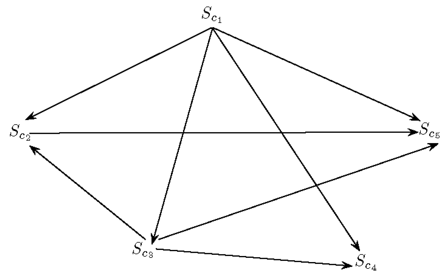
(xii). Finally, to rank the companies according to the outranking values of aggregated 4F linguistic dominance matrix T, we draw a directed graph for each pair of companies as shown in Figure 1.

From directed graph of companies as shown in Figure 1 the following cases arise.

• There exists directed edges from $S_{c_1}$ to $S_{c_2}$,$S_{c_3}$,$S_{c_4}$ and $S_{c_5}$ which show $S_{c_1}$ is preferred over all other companies according to its salary package.
• Similarly, $S_{c_1}$ is preferred over $S_{c_5}$.
• Similarly, $S_{c_3}$ is preferred over $S_{c_2}$,$S_{c_4}$ and $S_{c_5}$.
• There does not exist any edge from $S_{c_4}$ to any other company, which shows $S_{c_4}$ is incomparable to others.
• Similarly, $S_{c_5}$ is incomparable to others.

Hence, $S_{c_1}$ is the most dominated company as compared to others and has highest ranking according to its salary package.

We show the comparison of companies and summarize the whole procedure in

Table 6. Tabular representation of comparison of companies.

Comparison of Companies	${\mathit{Y}}_{\mathit{uv}}$	${\mathit{Z}}_{\mathit{uv}}$	${\mathit{y}}_{\mathit{uv}}$	${\mathit{z}}_{\mathit{uv}}$	${\mathit{r}}_{\mathit{uv}}$	${\mathit{s}}_{\mathit{uv}}$	${\mathit{t}}_{\mathit{uv}}$	$\mathit{Ranking}$
$(S_{c_1},S_{c_2})$	$\{1,3,4\}$	$\left\{2\right\}$	$0.81$	$0.3189$	1	1	1	$S_{c_1}\to S_{c_2}$
$(S_{c_1},S_{c_3})$	$\{3,4\}$	$\{1,2\}$	$0.66$	$0.6639$	1	1	1	$S_{c_1}\to S_{c_3}$
$(S_{c_1},S_{c_4})$	$\{1,3,4\}$	$\left\{2\right\}$	$0.81$	$0.6488$	1	1	1	$S_{c_1}\to S_{c_4}$
$(S_{c_1},S_{c_5})$	$\{1,3,4\}$	$\left\{2\right\}$	$0.81$	$0.8293$	1	1	1	$S_{c_1}\to S_{c_5}$
$(S_{c_2},S_{c_1})$	$\left\{2\right\}$	$\{1,3,4\}$	$0.19$	1	0	0	0	Incomparable
$(S_{c_2},S_{c_3})$	$\{2,4\}$	$\{1,3,4\}$	$0.58$	1	1	0	0	Incomparable
$(S_{c_2},S_{c_4})$	$\{1,3,4\}$	$\{1,3,4\}$	$0.81$	1	1	0	0	Incomparable
$(S_{c_2},S_{c_5})$	$\{3,4\}$	$\{1,2,4\}$	$0.66$	$0.6890$	1	1	1	$S_{c_2}\to S_{c_5}$
$(S_{c_3},S_{c_1})$	$\{1,2\}$	$\{3,4\}$	$0.34$	1	0	0	0	Incomparable
$(S_{c_3},S_{c_2})$	$\{1,2,3\}$	$\{2,4\}$	$0.61$	$0.7222$	1	1	1	$S_{c_3}\to S_{c_2}$
$(S_{c_3},S_{c_4})$	$\{1,3,4\}$	$\left\{2\right\}$	$0.81$	$0.5451$	1	1	1	$S_{c_3}\to S_{c_4}$
$(S_{c_3},S_{c_5})$	$\{1,3,4\}$	$\left\{2\right\}$	$0.81$	$0.4451$	1	1	1	$S_{c_3}\to S_{c_5}$
$(S_{c_4},S_{c_1})$	$\left\{2\right\}$	$\{1,3,4\}$	$0.19$	1	0	0	0	Incomparable
$(S_{c_4},S_{c_2})$	$\{2,3\}$	$\{1,3,4\}$	$0.46$	1	0	0	0	Incomparable
$(S_{c_4},S_{c_3})$	$\left\{2\right\}$	$\{1,3,4\}$	$0.19$	1	0	0	0	Incomparable
$(S_{c_4},S_{c_5})$	$\left\{3\right\}$	$\{1,2,4\}$	$0.27$	1	0	0	0	Incomparable
$(S_{c_5},S_{c_1})$	$\left\{2\right\}$	$\{1,3,4\}$	$0.19$	1	0	0	0	Incomparable
$(S_{c_5},S_{c_2})$	$\{1,2\}$	$\{3,4\}$	$0.34$	1	0	0	0	Incomparable
$(S_{c_5},S_{c_3})$	$\left\{2\right\}$	$\{1,3,4\}$	$0.19$	1	0	0	0	Incomparable
$(S_{c_5},S_{c_4})$	$\{1,2,4\}$	$\left\{3\right\}$	$0.73$	$0.9791$	1	0	0	Incomparable

.

4. $\mathit{m}$F Linguistic ELECTRE-I Approach for MCGDM

In this section, we introduce an mF linguistic ELECTRE-I approach for MCGDM problems, which is based on the concept of mFLV. We also apply this approach to real-life examples in Section 4.1, to show its importance and feasibility. In this approach, a group of r decision-makers ($D_g,g=1,2,\cdots ,r$) is responsible for evaluating mFLV of n different alternatives ($a_p\in A,p=1,2,\cdots ,n$) under k different linguistic values of $L_v$ ($V_l,l=1,2,\cdots ,k$). In the same sense as we used in MCDM, the degree of each alternative over all the linguistic values $V_l^{\prime }s$ is given by an mF set ${\wp }_p=\{(a_p,d_{pl}^{gi})|i=1,2,\cdots m\},$ where $d_{pl}^{gi}=p_i\circ d_{pl}^g(a_p,V_l)\in [0,1]$ and $d_{pl}^i$ classify the different properties or criteria of linguistic values according to each decision-maker.  

$(\mathbf{i}).$ In this case, a group of r decision-makers is responsible for evaluating mFLV of n different alternatives, and the suitable ratings of alternatives are according to all decision-makers that are assessed in terms of m different characteristics under the physical domain $P_d$. Tabular representation of $mF$ linguistic decision matrix under group of r decision-makers is given by

Table 7. Tabular representation of $mF$ linguistic decision matrix under a group of decision-makers.

	$\mathit{m}-$Polar Fuzzy	Physical Domain
Decision	Linguistic	${\mathit{P}}_{{\mathit{d}}_{\mathbf{1}}}$	${\mathit{P}}_{{\mathit{d}}_{\mathbf{2}}}$	⋯	${\mathit{P}}_{{\mathit{d}}_{\mathit{k}}}$
Makers	Variable	$\mathit{m}-$Polar Fuzzy Linguistic Values
	${\mathit{L}}_{\mathit{v}}$	${\mathit{V}}_{\mathbf{1}}$	${\mathit{V}}_{\mathbf{2}}$	⋯	${\mathit{V}}_{\mathit{k}}$
	$a_1$	$(d_{11}^{g1},d_{11}^{g2},\cdots ,d_{11}^{gm})$	$(d_{12}^{g1},d_{12}^{g2},\cdots ,d_{12}^{gm})$	⋯	$(d_{1k}^{g1},d_{1k}^{g2},\cdots ,d_{1k}^{gm})$
$D_g$	$a_2$	$(d_{21}^{g1},d_{21}^{g2},\cdots ,d_{21}^{gm})$	$(d_{22}^{g1},d_{22}^{g2},\cdots ,d_{22}^{gm})$	⋯	$(d_{2k}^{g1},d_{2k}^{g2},\cdots ,d_{2k}^{gm})$
	⋮	⋮	⋮	⋮	⋮
	$a_n$	$(d_{n1}^{g1},d_{n1}^{g2},\cdots ,d_{n1}^{gm})$	$(d_{n2}^{g1},d_{n2}^{g2},\cdots ,d_{n2}^{gm})$	⋯	$(d_{nk}^{g1},d_{nk}^{g2},\cdots ,d_{nk}^{gm})$

, which describes the ratings given by each decision-maker.

Table 7 shows the different ratings of linguistic values assigned by a group of r decision-makers, in which each decision-maker assigns ratings according to his choice. The final $mF$ linguistic decision matrix under group of decision-makers is the aggregated $mF$ linguistic decision matrix that is the average ratings of all decision-makers. Aggregated ratings are calculated as follows:

$$d_{pl}^{1^{\prime }}=\frac{1}{r}{\displaystyle \sum _{g=1}^r}{d}_{pl}^{g1},d_{pl}^{2^{\prime }}=\frac{1}{r}{\displaystyle \sum _{g=1}^r}{d}_{pl}^{g2},\cdots ,d_{pl}^{m^{\prime }}=\frac{1}{r}{\displaystyle \sum _{g=1}^r}{d}_{pl}^{gm}.$$

$$p=1,2,\cdots ,n \mathrm{and} l=1,2,\cdots ,k.$$

For final decisions and ratings, aggregated $mF$ linguistic decision matrix is calculated in

Table 8. Tabular representation of aggregated $mF$ linguistic decision matrix.

$\mathit{m}-$Polar Fuzzy	Physical Domain
Linguistic	${\mathit{P}}_{{\mathit{d}}_1}$	${\mathit{P}}_{{\mathit{d}}_2}$	⋯	${\mathit{P}}_{{\mathit{d}}_{\mathit{k}}}$
Variable	$\mathit{m}-$Polar Fuzzy Linguistic Values and Weights
${\mathit{L}}_{\mathit{v}}$	${\mathit{V}}_{\mathbf{1}}$	${\mathit{V}}_{\mathbf{2}}$	⋯	${\mathit{V}}_{\mathit{k}}$
	${\mathit{w}}_{\mathbf{1}}$	${\mathit{w}}_{\mathbf{2}}$	⋯	${\mathit{w}}_{\mathit{k}}$
$a_1$	$(d_{11}^{1^{\prime }},d_{11}^{2^{\prime }},\cdots ,d_{11}^{m^{\prime }})$	$(d_{12}^{1^{\prime }},d_{12}^{2^{\prime }},\cdots ,d_{12}^{m^{\prime }})$	⋯	$(d_{1k}^{1^{\prime }},d_{1k}^{2^{\prime }},\cdots ,d_{1k}^{m^{\prime }})$
$a_2$	$(d_{21}^{1^{\prime }},d_{21}^{2^{\prime }},\cdots ,d_{21}^{m^{\prime }})$	$(d_{22}^{1^{\prime }},d_{22}^{2^{\prime }},\cdots ,d_{22}^{m^{\prime }})$	⋯	$(d_{2k}^{1^{\prime }},d_{2k}^{2^{\prime }},\cdots ,d_{2k}^{m^{\prime }})$
⋮	⋮	⋮	⋮	⋮
$a_n$	$(d_{n1}^{1^{\prime }},d_{n1}^{2^{\prime }},\cdots ,d_{n1}^{m^{\prime }})$	$(d_{n2}^{1^{\prime }},d_{n2}^{2^{\prime }},\cdots ,d_{n2}^{m^{\prime }})$	⋯	$(d_{nk}^{1^{\prime }},d_{nk}^{2^{\prime }},\cdots ,d_{nk}^{m^{\prime }})$

by using above-average ratings.

$(\mathbf{ii}).$ Decision-makers have an authority to assign weights to each linguistic value of alternatives according to their choice and the importance of each linguistic value, but we are discussing the case of mFLV so decision-makers have to assign the weights in terms of the linguistic term set $L=\{{\mathrm{L}}_1=\mathrm{extremely}\mathrm{low},{\mathrm{L}}_2=\mathrm{medium},\cdots ,{\mathrm{L}}_{\mathrm{k}}=\mathrm{very}\mathrm{high}\}$. We suppose that the weights assigned by the decision-makers are

$$W^g=(w_1^g,w_2^g,\cdots ,w_k^g)\in (0,1],g=1,2,\cdots ,r.$$

Weights assigned by the decision-makers satisfy the normalized condition. i.e.,

$${\displaystyle \sum _{l=1}^k}{w}_l^g=1,g=1,2,\cdots ,r.$$

Aggregated weights according to decision-makers are $W^{{}^{\prime }}=(w_1^{{}^{\prime }},w_2^{{}^{\prime }},\cdots ,w_k^{{}^{\prime }}),$ where,

$$w_l^{{}^{\prime }}=\frac{1}{r}{\displaystyle \sum _{g=1}^r}{w}_l^g,l=1,2,\cdots ,k.$$

$(\mathbf{iii}).$ The weighted aggregated $mF$ linguistic decision matrix $W={[(e_{pl}^{1^{\prime }},e_{pl}^{2^{\prime }},\cdots ,e_{pl}^{m^{\prime }})]}_{n\times k}$ under group decision-making is calculated as

$$e_{pl}^{1^{\prime }}=w_l^{{}^{\prime }}{d}_{pl}^{1^{\prime }},e_{pl}^{2^{\prime }}=w_l^{{}^{\prime }}{d}_{pl}^{2^{\prime }},\cdots ,e_{pl}^{m^{\prime }}=w_l^{{}^{\prime }}{d}_{pl}^{m^{\prime }}.$$

Steps $(\mathbf{iv})$ to $(\mathbf{xii})$ are same as described in Section 3.

4.1. Selection of Corrupted Country

Usually, corruption is considered to be criminal activity or dishonesty initiated by a person or organization associated with the situation of authority, often to attain unauthorized benefits. Corruption may comprise several activities including misappropriation, extortion, and bribery, though it may also involve practices that are enforced in several countries. Corruption can appear on variant scales. It ranges from poor level of consideration between a small number of people—“petty corruption”—to the corruption that influences the government on a large scale—“grand corruption”—and corruption that is so common it is part of the everyday conformation of society, carrying corruption as one of the evidences of organized crime. Crime and corruption are regional, sociological junctures which occur with usual constancy in all countries on a global scale in fluctuating proportions and degrees. Increasingly, several tools and intimators have been developed that can rate several forms of corruption with growing accuracy.

• Petty corruption

Petty corruption appears at a lower scale and occurs at the practical end of civil services when a civil authoritative person accommodates civil people. For example, in several small places such as police stations, registration offices, state licensing boards, and several other government and private sectors, it indicates the daily fault of power by low- and mid-level public officials in their interactions with frequent civilians, who are trying to approach basic services or goods in public places such as schools, police departments, hospitals, and other agencies.

• Grand corruption

Grand corruption occurs at the highest scale of government in a way that depends on the expressive overthrow of the legal, political, and economic systems. Such a type of corruption is usually found in countries with dictatorial or authoritarian governments but also in those without sufficient policing of corruption.

• Systemic corruption

Systemic corruption or endemic corruption is primarily due to the weaknesses of an institution, organization, or management. It can be differentiated with agents or individual officials, who perform corruptly within the system. Factors that encourage systemic corruption include elective powers, lack of transparency, conflicting stimulus, monopolistic powers, low pay, and a culture of immunity. Measuring the corruption at country level is a very difficult phenomenon for anti-corruption agencies because it is willfully hidden, and therefore it is almost impossible to evaluate it directly. Corruption inside a rustic government undermines the solidity of its establishments and tends to cause popular unrest. To overcome this difficulty and to measure the corruption at country level, we use mF linguistic ELECTRE-I approach for MCGDM, in which corruption is the linguistic variable and $C=\{C_1,C_2,C_3,C_4,C_5,C_6,C_7\}$ is the set of seven countries in which corruption must be measured. Let $V=\{\mathrm{petty}\mathrm{corruption},\mathrm{grand}\mathrm{corruption},\mathrm{systemic}\mathrm{corruption}\}$ be the set of linguistic values of corruption. Anti-corruption agencies and media sources work as decision-makers; they have to evaluate the countries on the basis of the linguistic values of corruption and design a physical domain in which corruption takes its quantitative values, i.e., $P_d=[10\%,100\%].$ The physical domain for linguistic values of corruption is given as follows:

• For petty corruption, physical domain is $40\%$–$60\%$,
• For grand corruption, physical domain is $50\%$–$80\%$,
• For systemic corruption, physical domain is $30\%$–$70\%$.

Physical domain of each linguistic value shows the scale of corruption given by group of decision-makers. The degree of corruption of each country over all the linguistic values are given by 4F set ${\wp }_p=\left\{(C_p,d_{pl}^i)\right|i=1,2,3,4\},$ where

• $d_{pl}^1=p_1\circ d_{pl}(a_p,V_l)$ serves for personal greed,
• $d_{pl}^2=p_2\circ d_{pl}(a_p,V_l)$ serves for cultural environment,
• $d_{pl}^3=p_3\circ d_{pl}(a_p,V_l)$ serves for Institutional scale,
• $d_{pl}^4=p_4\circ d_{pl}(a_p,V_l)$ serves for organizational level,

where $p=1,2,\cdots ,7,$ and $l=1,2,3.$ The 4F set shows the further criteria or properties on which linguistic values depend.

(i). Tabular representation of 4F linguistic group decision matrix is given by

Table 9. Tabular representation of 4F linguistic group decision matrix for corruption.

	$4-$Polar Fuzzy	Physical Domain
Decision	Linguistic	40%–60%	50%–80%	30%–70%
Makers	Variable	$\mathbf{4}-$Polar Fuzzy Linguistic Values
	(Corruption)	Petty Corruption	Grand Corruption	Systemic Corruption
Ratings according to anti-corruption agencies
	$C_1$	(0.6,0.5,0.3,0.4)	(0.5,0.6,0.7,0.8)	(0.2,0.1,0.5,0.6)
	$C_2$	(0.5,0.7,0.5,0.6)	(0.4,0.6,0.8,0.9)	(0.3,0.4,0.7,0.8)
	$C_3$	(0.3,0.4,0.4,0.7)	(0.6,0.5,0.7,0.8)	(0.3,0.3,0.5,0.7)
$D_1$	$C_4$	(0.3,0.6,0.5,0.4)	(0.7,0.6,0.8,0.7)	(0.2,0.4,0.4,0.6)
	$C_5$	(0.4,0.4,0.5,0.7)	(0.4,0.5,0.8,0.8)	(0.1,0.4,0.3,0.5)
	$C_6$	(0.6,0.4,0.5,0.7)	(0.6,0.7,0.5,0.7)	(0.5,0.5,0.4,0.7)
	$C_7$	(0.7,0.3,0.2,0.5)	(0.4,0.5,0.6,0.8)	(0.4,0.3,0.5,0.8)
Ratings according to media sources
	$C_1$	(0.5,0.4,0.3,0.5)	(0.6,0.6,0.8,0.6)	(0.3,0.2,0.6,0.7)
	$C_2$	(0.6,0.4,0.5,0.7)	(0.8,0.7,0.7,0.8)	(0.4,0.3,0.7,0.6)
	$C_3$	(0.3,0.5,0.7,0.6)	(0.4,0.5,0.6,0.8)	(0.5,0.4,0.6,0.6)
$D_2$	$C_4$	(0.5,0.6,0.5,0.3)	(0.5,0.7,0.6,0.8)	(0.3,0.5,0.6,0.5)
	$C_5$	(0.5,0.6,0.5,0.7)	(0.7,0.4,0.7,0.7)	(0.3,0.4,0.5,0.4)
	$C_6$	(0.7,0.4,0.4,0.5)	(0.6,0.6,0.6,0.6)	(0.4,0.3,0.6,0.5)
	$C_7$	(0.6,0.5,0.3,0.5)	(0.5,0.7,0.7,0.6)	(0.4,0.4,0.7,0.7)

. It shows the different ratings of linguistic values assigned by a group of two decision-makers, in which each decision-maker assigns ratings according to his choice.

For final decision and ratings, aggregated 4F linguistic decision matrix is calculated in

Table 10. Tabular representation of aggregated 4F linguistic group decision matrix for corruption.

$4-$Polar Fuzzy	Physical Domain
Linguistic	40%–60%	50%–80%	30%–70%
Variable	$\mathbf{4}-$Polar Fuzzy Linguistic Values
(Corruption)	Petty Corruption	Grand Corruption	Systemic Corruption
$C_1$	(0.55,0.45,0.3,0.45)	(0.55,0.6,0.75,0.7)	(0.25,0.15,0.55,0.65)
$C_2$	(0.55,0.55,0.5,0.65)	(0.6,0.65,0.75,0.85)	(0.35,0.35,0.7,0.7)
$C_3$	(0.3,0.45,0.55,0.65)	(0.5,0.5,0.65,0.8)	(0.4,0.35,0.55,0.65)
$C_4$	(0.4,0.6,0.5,0.35)	(0.6,0.65,0.7,0.75)	(0.25,0.45,0.5,0.55)
$C_5$	(0.45,0.5,0.5,0.7)	(0.55,0.45,0.75,0.75)	(0.2,0.4,0.4,0.45)
$C_6$	(0.65,0.4,0.45,0.6)	(0.6,0.65,0.55,0.65)	(0.45,0.4,0.5,0.6)
$C_7$	(0.65,0.4,0.25,0.5)	(0.45,0.6,0.65,0.7)	(0.4,0.35,0.6,0.75)

.

(ii). To measure the corruption at country level, anti-corruption agencies and media sources are considered as decision-makers and the weights assigned by decision-makers are given by

Table 11. Tabular representation of weights assigned by decision-makers.

Decision	$4-$Polar Fuzzy Linguistic Values
Makers	Petty Corruption	Grand Corruption	Systemic Corruption
$D_1$	0.3251	0.3453	0.3296
$D_2$	0.2915	0.3801	0.3284
$D^{{}^{\prime }}$	0.3083	0.3627	0.3290

.

(iii). The weighted aggregated 4F linguistic group decision matrix is calculated in

Table 12. Tabular representation of weighted aggregated 4F linguistic group decision matrix for corruption.

$4-$Polar Fuzzy	Physical Domain
Linguistic	40%–60%	50%–80%	30%–70%
Variable	$4-$Polar Fuzzy Linguistic Values
(Corruption)	Petty Corruption	Grand Corruption	Systemic Corruption
$C_1$	(0.1696,0.1387,0.0925,0.1387)	(0.1995,0.2176,0.2720,0.2539)	(0.0823,0.0494,0.1810,0.2138)
$C_2$	(0.1696,0.1696,0.1542,0.2004)	(0.2176,0.2358,0.2720,0.3083)	(0.1152,0.1152,0.2303,0.2303)
$C_3$	(0.0925,0.1387,0.1696,0.2004)	(0.1814,0.1814,0.2358,0.2902)	(0.1316,0.1152,0.1810,0.2138)
$C_4$	(0.1233,0.1850,0.1542,0.1079)	(0.2176,0.2358,0.2539,0.2720)	(0.0823,0.1481,0.1645,0.1810)
$C_5$	(0.1387,0.1542,0.1542,0.2158)	(0.1995,0.1632,0.2720,0.2720)	(0.0658,0.1316,0.1316,0.1481)
$C_6$	(0.2004,0.1233,0.1387,0.1850)	(0.2176,0.2358,0.1995,0.2358)	(0.1481,0.1316,0.1645,0.1974)
$C_7$	(0.2004,0.1233,0.0771,0.1542)	(0.1632,0.2176,0.2358,0.2539)	(0.1316,0.1152,0.2139,0.2468)

.

(iv). A 4F linguistic concordance set is calculated in

Table 13. Tabular representation of 4F linguistic concordance set.

v	1	2	3	4	5	6	7
$Y_{1v}$	−	$\left\{\right\}$	$\left\{2\right\}$	$\left\{\right\}$	$\{2,3\}$	$\left\{2\right\}$	$\left\{2\right\}$
$Y_{2v}$	$\{1,2,3\}$	−	$\{1,2,3\}$	$\{1,2,3\}$	$\{1,2,3\}$	$\{1,2,3\}$	$\{1,2,3\}$
$Y_{3v}$	$\{1,3\}$	$\left\{\right\}$	−	$\{1,3\}$	$\left\{3\right\}$	$\{2,3\}$	$\{1,2\}$
$Y_{4v}$	$\{1,2,3\}$	$\left\{\right\}$	$\left\{2\right\}$	−	$\{2,3\}$	$\left\{2\right\}$	$\{1,2\}$
$Y_{5v}$	$\left\{1\right\}$	$\left\{\right\}$	$\{1,2\}$	$\left\{1\right\}$	−	$\{1,2\}$	$\{1,2\}$
$Y_{6v}$	$\{1,3\}$	$\left\{\right\}$	$\{1,2,3\}$	$\{1,3\}$	$\left\{3\right\}$	−	$\{1,2\}$
$Y_{7v}$	$\{1,3\}$	$\left\{3\right\}$	$\left\{3\right\}$	$\left\{3\right\}$	$\left\{3\right\}$	$\left\{3\right\}$	−

.

(v). A 4F linguistic discordance set is calculated in

Table 14. Tabular representation of 4F linguistic discordance set.

v	1	2	3	4	5	6	7
$Z_{1v}$	−	$\{1,2,3\}$	$\{1,3\}$	$\{1,2,3\}$	$\left\{1\right\}$	$\{1,3\}$	$\{1,3\}$
$Z_{2v}$	$\left\{\right\}$	−	$\left\{\right\}$	$\left\{\right\}$	$\left\{\right\}$	$\left\{\right\}$	$\left\{3\right\}$
$Z_{3v}$	$\left\{2\right\}$	$\{1,2,3\}$	−	$\left\{2\right\}$	$\{1,2\}$	$\{1,2,3\}$	$\left\{3\right\}$
$Z_{4v}$	$\left\{\right\}$	$\{1,2,3\}$	$\{1,3\}$	−	$\left\{1\right\}$	$\{1,3\}$	$\left\{3\right\}$
$Z_{5v}$	$\{2,3\}$	$\{1,2,3\}$	$\left\{3\right\}$	$\{2,3\}$	−	$\left\{3\right\}$	$\left\{3\right\}$
$Z_{6v}$	$\left\{2\right\}$	$\{1,2,3\}$	$\{2,3\}$	$\left\{2\right\}$	$\{1,2\}$	−	$\left\{3\right\}$
$Z_{7v}$	$\left\{2\right\}$	$\{1,2,3\}$	$\{1,2\}$	$\{1,2\}$	$\{1,2\}$	$\{1,2\}$	−

.

(vi). A 4F linguistic concordance matrix is calculated as follows:

$$Y=\left(\begin{array}{ccccccc}-& 0& 0.3627& 0& 0.6917& 0.3627& 0.3627\\ 1& -& 1& 1& 1& 1& 1\\ 0.6373& 0& -& 0.6373& 0.3290& 0.6917& 0.6710\\ 1& 0& 0.3627& -& 0.6917& 0.3627& 0.6710\\ 0.3083& 0& 0.6710& 0.3083& -& 0.6710& 0.6710\\ 0.6373& 0& 1& 0.6373& 0.3290& -& 0.6710\\ 0.6373& 0.3290& 0.3290& 0.3290& 0.3290& 0.3290& -\end{array}\right).$$

(vii). A 4F linguistic discordance matrix is calculated as follows:

$$Z=\left(\begin{array}{ccccccc}-& 1& 1& 1& 0.8900& 1& 1\\ 0& -& 0& 0& 0& 0& 0.3813\\ 0.5221& 1& -& 0.644& 0.5009& 1& 0.2448\\ 0& 1& 1& -& 1& 1& 0.7079\\ 1& 1& 1& 0.6792& -& 0.9193& 1\\ 0.7328& 1& 0.8089& 0.5182& 1& -& 0.9071\\ 0.5693& 1& 1& 1& 0.8811& 1& -\end{array}\right).$$

(viii). A 4F linguistic concordance level $\overline{y}=0.5243$, and 4F linguistic discordance level $\overline{z}=0.7359$ are calculated.

(ix). A 4F linguistic concordance dominance matrix is calculated as follows:

$$R=\left(\begin{array}{ccccccc}-& 0& 0& 0& 1& 0& 0\\ 1& -& 1& 1& 1& 1& 1\\ 1& 0& -& 1& 0& 1& 1\\ 1& 0& 0& -& 1& 0& 1\\ 0& 0& 1& 0& -& 1& 1\\ 1& 0& 1& 1& 0& -& 1\\ 1& 0& 0& 0& 0& 0& -\end{array}\right).$$

(x). A 4F linguistic discordance dominance matrix is calculated as follows:

$$S=\left(\begin{array}{ccccccc}-& 0& 0& 0& 0& 0& 0\\ 1& -& 1& 1& 1& 1& 1\\ 1& 0& -& 1& 1& 0& 1\\ 1& 0& 0& -& 0& 0& 1\\ 0& 0& 0& 1& -& 0& 0\\ 1& 0& 0& 1& 0& -& 0\\ 1& 0& 0& 0& 0& 0& -\end{array}\right).$$

(xi). An aggregated 4F linguistic dominance matrix is calculated as follows:

$$T=\left(\begin{array}{ccccccc}-& 0& 0& 0& 0& 0& 0\\ 1& -& 1& 1& 1& 1& 1\\ 1& 0& -& 1& 0& 0& 1\\ 1& 0& 0& -& 0& 0& 1\\ 0& 0& 0& 0& -& 0& 0\\ 1& 0& 0& 1& 0& -& 0\\ 1& 0& 0& 0& 0& 0& -\end{array}\right).$$

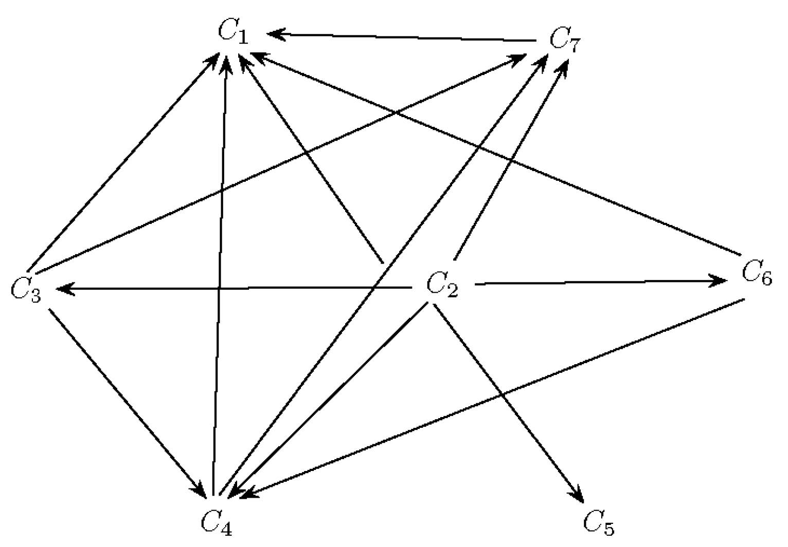
(xii). Finally, to rank the companies according to the outranking values of aggregated 4F linguistic dominance matrix T, we draw a directed graph for each pair of countries as shown in Figure 2.

From directed graph of countries as shown in Figure 2 the following cases arise.

• There does not exist any edge from $C_1$ to any other country, which shows $C_1$ is incomparable to others.
• There exists directed edges from $C_2$ to $C_1$, $C_3$, $C_4$, $C_5$, $C_6$ and $C_7$ which show $C_2$ is preferred over all other countries.
• Similarly, $C_3$ is preferred over $C_1$, $C_4$ and $C_7$.
• Similarly, $C_4$ is preferred over $C_1$ and $C_7$.
• There does not exist any edge from $C_5$ to any other country, which shows $S{C}_5$ is incomparable to others.
• $C_6$ is preferred over $C_1$ and $C_4$.
• Similarly, $C_7$ is preferred over $C_1$.

Hence, the country $C_2$ is most dominated as compared to others. Hence $C_2$ is the most corrupted country.

We show the comparison of countries and summarize the whole procedure in

Table 15. Tabular representation of comparison of countries.

Comparison of Countries	${\mathit{Y}}_{\mathit{uv}}$	${\mathit{Z}}_{\mathit{uv}}$	${\mathit{y}}_{\mathit{uv}}$	${\mathit{z}}_{\mathit{uv}}$	${\mathit{r}}_{\mathit{uv}}$	${\mathit{s}}_{\mathit{uv}}$	${\mathit{t}}_{\mathit{uv}}$	$\mathit{Ranking}$
$(C_1,C_2)$	$\left\{\right\}$	$\{1,2,3\}$	0	1	0	0	0	Incomparable
$(C_1,C_3)$	$\left\{2\right\}$	$\{1,3\}$	$0.3627$	1	0	0	0	Incomparable
$(C_1,C_4)$	$\left\{\right\}$	$\{1,2,3\}$	0	1	0	0	0	Incomparable
$(C_1,C_5)$	$\{2,3\}$	$\left\{1\right\}$	$0.6917$	1	1	0	0	Incomparable
$(C_1,C_6)$	$\left\{2\right\}$	$\{1,3\}$	$0.3627$	1	0	0	0	Incomparable
$(C_1,C_7)$	$\left\{2\right\}$	$\{1,3\}$	$0.3627$	1	0	0	0	Incomparable
$(C_2,C_1)$	$\{1,2,3\}$	$\left\{\right\}$	1	0	1	1	1	$C_2\to C_1$
$(C_2,C_3)$	$\{1,2,3\}$	$\left\{\right\}$	1	0	1	1	1	$C_2\to C_3$
$(C_2,C_4)$	$\{1,2,3\}$	$\left\{\right\}$	1	0	1	1	1	$C_2\to C_4$
$(C_2,C_5)$	$\{1,2,3\}$	$\left\{\right\}$	1	0	1	1	1	$C_2\to C_5$
$(C_2,C_6)$	$\{1,2,3\}$	$\left\{\right\}$	1	0	1	1	1	$C_2\to C_6$
$(C_2,C_7)$	$\{1,2,3\}$	$\left\{3\right\}$	1	$0.3813$	1	1	1	$C_2\to C_7$
$(C_3,C_1)$	$\{1,3\}$	$\left\{2\right\}$	$0.6373$	$0.5221$	1	1	1	$C_3\to C_1$
$(C_3,C_2)$	$\left\{\right\}$	$\{1,2,3\}$	0	1	0	0	0	Incomparable
$(C_3,C_4)$	$\{1,3\}$	$\left\{2\right\}$	$0.6373$	$0.6444$	1	1	1	$C_3\to C_4$
$(C_3,C_5)$	$\left\{3\right\}$	$\{1,2\}$	$0.3290$	$0.5009$	0	1	0	Incomparable
$(C_3,C_6)$	$\{2,3\}$	$\{1,2,3\}$	$0.6917$	1	1	0	0	Incomparable
$(C_3,C_7)$	$\{1,2\}$	$\left\{3\right\}$	$0.6710$	$0.2448$	1	1	1	$C_3\to C_7$
$(C_4,C_1)$	$\{1,2,3\}$	$\left\{\right\}$	1	0	1	1	1	$C_4\to C_1$
$(C_4,C_2)$	$\left\{\right\}$	$\{1,2,3\}$	0	1	0	0	0	Incomparable
$(C_4,C_3)$	$\left\{2\right\}$	$\{1,3\}$	$0.3627$	1	0	0	0	Incomparable
$(C_4,C_5)$	$\{2,3\}$	$\left\{1\right\}$	$0.6917$	1	1	0	0	Incomparable
$(C_4,C_6)$	$\left\{2\right\}$	$\{1,3\}$	$0.3627$	1	0	0	0	Incomparable
$(C_4,C_7)$	$\{1,2\}$	$\left\{3\right\}$	$0.6710$	$0.7079$	1	1	1	$C_4\to C_7$
$(C_5,C_1)$	$\left\{1\right\}$	$\{2,3\}$	$0.3083$	1	0	0	0	Incomparable
$(C_5,C_2)$	$\left\{\right\}$	$\{1,2,3\}$	0	1	0	0	0	Incomparable
$(C_5,C_3)$	$\{1,2\}$	$\left\{3\right\}$	$0.6710$	1	1	0	0	Incomparable
$(C_5,C_4)$	$\left\{1\right\}$	$\{2,3\}$	$0.3083$	$0.6792$	0	1	0	Incomparable
$(C_5,C_6)$	$\{1,2\}$	$\left\{3\right\}$	$0.6710$	$0.9193$	1	0	0	Incomparable
$(C_5,C_7)$	$\{1,2\}$	$\left\{3\right\}$	$0.6710$	1	1	0	0	Incomparable
$(C_6,C_1)$	$\{1,3\}$	$\left\{2\right\}$	$0.6373$	$0.7328$	1	1	1	$C_6\to C_1$
$(C_6,C_2)$	$\left\{\right\}$	$\{1,2,3\}$	0	1	0	0	0	Incomparable
$(C_6,C_3)$	$\{1,2,3\}$	$\{2,3\}$	1	$0.8089$	1	0	0	Incomparable
$(C_6,C_4)$	$\{1,3\}$	$\left\{2\right\}$	$0.6373$	$0.5182$	1	1	1	$C_6\to C_4$
$(C_6,C_5)$	$\left\{3\right\}$	$\{1,2\}$	$0.3290$	1	0	0	0	Incomparable
$(C_6,C_7)$	$\{1,2\}$	$\left\{3\right\}$	$0.6710$	$0.9071$	1	0	0	Incomparable
$(C_7,C_1)$	$\{1,3\}$	$\left\{2\right\}$	$0.6373$	$0.5693$	1	1	1	$C_7\to C_1$
$(C_7,C_2)$	$\left\{3\right\}$	$\{1,2,3\}$	$0.3290$	1	0	0	0	Incomparable
$(C_7,C_3)$	$\left\{3\right\}$	$\{1,2\}$	$0.3290$	1	0	0	0	Incomparable
$(C_7,C_4)$	$\left\{3\right\}$	$\{1,2\}$	$0.3290$	1	0	0	0	Incomparable
$(C_7,C_5)$	$\left\{3\right\}$	$\{1,2\}$	$0.3290$	$0.8811$	0	0	0	Incomparable
$(C_7,C_6)$	$\left\{3\right\}$	$\{1,2\}$	$0.3290$	1	0	0	0	Incomparable

.

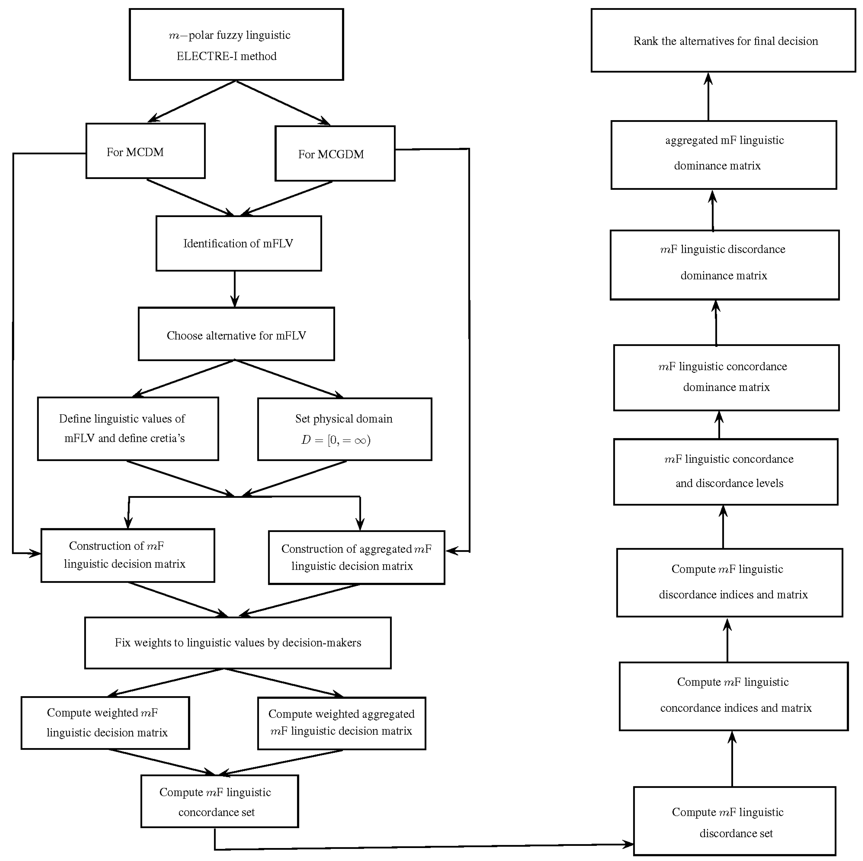
We present our proposed method of decision-making in an Algorithm 1 and show its flow chart in Figure 3.

Algorithm 1: The algorithm of proposed approach for MCGDM.

Step 1. Input n, no. of alternatives against linguistic variable. k, no. of linguistic values. m, no. of membership values. g, no. of decision-makers. $D_g$, mF linguistic decision matrices according to decision-makers. $w_l^g$, weights according to decision-makers. Step 2. Compute an aggregated mF linguistic decision matrix D. Step 3. Compute aggregated weights $W^{{}^{\prime }}$. Step 4. Compute the weighted aggregated mF linguistic decision matrix W. Step 5. Compute mF linguistic concordance set $Y_{uv}$. Step 6. Compute mF linguistic discordance set $Z_{uv}$. Step 7. Compute mF linguistic concordance indices $y_{uv}$ and concordance matrix Y. Step 8. Compute mF linguistic discordance indices $z_{uv}$ and discordance matrix Z. Step 9. Compute mF linguistic concordance and discordance levels $\overline{y}$ and $\overline{z}$. Step 10. Compute mF linguistic concordance dominance matrix R. Step 11. Compute mF linguistic discordance dominance matrix S. Step 12. Compute aggregated mF linguistic dominance matrix T. Step 13. Output The most dominating alternative with maximum value of T.

5. Discussion of Proposed Approach

In this section, we discuss the novelty of our purposed concept and its decision-making methods.

• Linguistic variables are considered to be the generalizations of numerical variables and take the concept of words in natural languages as values and associate human knowledge into various systems in an organized, efficient and productive manner. In many applications of decision-making, where the situations totally depend upon uncertainty and imprecision, fuzzy linguistic variables are used extensively. All previously defined concepts related to linguistic variables are insufficient for explaining the situation, when the given data is in the form of sentences and words with m different numeric and fuzzy values within its crisp domain. It is actually the generalization of fuzzy linguistic variables, because in the proposed concept the linguistic values are further characterized into m different numeric and fuzzy values.
• ELECTRE-I method is preferred over all other MCDM methods, because it is a binary outranking method in which the alternatives can be compared without consideration of their fine preference. It is more reliable as it does not depend on expert personal opinions, and alternatives can be eliminated that are dominated by other alternatives to a specified degree.
• The comparison of mF linguistic variable and mF linguistic ELECTRE-I method with fuzzy linguistic approaches and decision-making methods given in the literature is described by an example of salary analysis of companies given in Section 3.1. In this example, we consider salary as a linguistic variable and define its linguistic values such as low, moderate, good, and very good; we call it 4F linguistic variable because we categorize these linguistic values in a further four different fuzzy values such as career, labor market, experience, and credential. Previous knowledge tells us about the linguistic values of a linguistic variable, but it is unable to deal the criteria on which linguistic values depend. An mF linguistic variable covers all the aspects on which salary is based and an mF linguistic ELECTRE-I approach can deal with such a complex situation and provides flexible decision results.

6. Conclusions

ELECTRE has been considered to be one of the MCDM techniques, based on the outranking relations, which has induced a new preference relation called incomparability used to handle situations in which the decision-makers are unable to compare two alternatives. Traditional methods are deemed ineffectual for studying the imprecise behavior of linguistic computations and assessments, because it has become difficult to collect data about linguistic assessments in terms of numeric and fuzzy values. To deal with such a complexity, we have proposed the concept of mFLV, which can deal with the situation when we have data in terms of linguistic assessments and m different numeric or fuzzy values as well. We also have developed an mF linguistic ELECTRE-I approach to deal with MCDM and MCGDM problems, which are used to handle complex situations of mFLV and compile the outranking relations of alternatives to choose and compare the best alternatives, among others. The mF linguistic ELECTRE-I method is used to get more authentic and consistent results, when we must eliminate the choices and to deal with the systems with more than one arrangement. Moreover, the proposed method is considered more efficient than previously existing methods, when the alternatives are eliminated that are dominated by other alternatives to a specified degree with linguistic values. However, the proposed approach is unable to determine and describe the weights assigned by decision-makers, although the weights considered in this approach are normalized but arbitrary. Finally, we have applied our technique to real-life problems, developed an algorithm, presented its flow chart, and generated computer programming code. In the future, we plan to extend our research study to MCDM and MCGDM methods such as PROMETHEE, AHP, and other versions of ELECTRE based on mFLV.

References

1. Dubois, D.; Prade, H. Fuzzy Sets and Systems: Theory and Applications; Kluwer: New York, NY, USA, 1980. [Google Scholar]
2. Zadeh, L.A. Fuzzy sets. Inf Control 1965, 8, 338–353. [Google Scholar] [CrossRef]
3. Torra, V.; Narukawa, Y. On hesitant fuzzy sets and decisions. IEEE Int. Conf. Fuzzy Syst. 2009, 1–3, 1378–1382. [Google Scholar]
4. Zhang, W.-R. Bipolar fuzzy sets and relations: A computational framework forcognitive modeling and multiagent decision analysis. Proc. IEEE Conf. 1994, 305–309. [Google Scholar] [CrossRef]
5. Chen, J.; Li, S.; Ma, S.; Wang, X. m—Polar fuzzy sets: An extension of bipolar fuzzy sets. Sci. World J. 2014, 2014, 416530. [Google Scholar] [CrossRef]
6. Akram, M. m—Polar fuzzy graphs-theory, methods & applications. Stud. Fuzziness Soft Comput. 2019, 371, 1–284. [Google Scholar]
7. Zadeh, L.A. The concept of a linguistic variable and its application to approximate reasoning, part I. Inf. Sci. 1975, 8, 199–249. [Google Scholar] [CrossRef]
8. Zadeh, L.A. The concept of a linguistic variable and its application to approximate reasoning, part II. Inf. Sci. 1975, 8, 301–357. [Google Scholar] [CrossRef]
9. Zadeh, L.A. The concept of a linguistic variable and its application to approximate reasoning, part III. Inf. Sci. 1975, 9, 43–80. [Google Scholar] [CrossRef]
10. RodrA-guez, R.M.; MartA-nez, L.; Herrera, F. A group decision-making model dealing with comparative linguistic expressions based on hesitant fuzzy linguistic term sets. Inf. Sci. 2013, 241, 28–42. [Google Scholar] [CrossRef]
11. Herrera, F.; Herrera-Viedma, E. Linguistic decision analysis: Steps for solving decision problems under linguistic information. Fuzzy Sets Syst. 2000, 115, 67–82. [Google Scholar] [CrossRef]
12. Herrera, F.; Herrera-Viedma, E.; Martinez, L. A fusion approach for managing multi-granularity linguistic term sets in decision making. Fuzzy Sets Syst. 2000, 114, 43–58. [Google Scholar] [CrossRef]
13. Meng, F.; Chen, X.; Zhang, Q. Multi-attribute decision analysis under a linguistic hesitant fuzzy environment. Inf. Sci. 2014, 267, 287–305. [Google Scholar] [CrossRef]
14. Ren, F.; Kong, M.; Pei, Z. A new hesitant fuzzy linguistic TOPSIS method for group multi-criteria linguistic decision-making. Symmetry 2017, 9, 289. [Google Scholar] [CrossRef]
15. Wang, R.C.; Chuu, S.J. Group decision-making using a fuzzy linguistic approach for evaluating the flexibility in a manufacturing system. Eur. J. Oper. Res. 2004, 154, 563–572. [Google Scholar] [CrossRef]
16. Herrera, F.; Alonso, S.; Chiclana, F.; Herrera-Viedma, E. Computing with words in decision-making: Foundations, trends and prospects. Fuzzy Opt. Decis. Mak. 2009, 8, 337–364. [Google Scholar] [CrossRef]
17. Mendel, J.M.; Zadeh, L.A.; Trillas, E.; Yager, R.; Lawry, J.; Hagras, H.; Guadarrama, S. What computing with words means to me [discussion forum]. IEEE Comput. Intell. Mag. 2010, 5, 20–26. [Google Scholar] [CrossRef]
18. Liu, P.D.; Su, Y. The extended TOPSIS based on trapezoid fuzzy linguistic variables. J. Converg. Inf. Technol. 2010, 5, 38–53. [Google Scholar]
19. Selvachandran, G.; Salleh, A.R. Intuitionistic fuzzy linguistic variables and intuitionistic fuzzy hedges. Far East J. Math. Sci. 2014, 95, 221–233. [Google Scholar]
20. Liao, H.C.; Xu, Z.S.; Zeng, X.J. Distance and similarity measures for hesitant fuzzy linguistic term sets and their application in multi-criteria decision-making. Inf. Sci. 2014, 271, 125–142. [Google Scholar] [CrossRef]
21. Riera, J.V.; Massanet, S.; Herrera-Viedma, E.; Torrens, J. Some interesting properties of the fuzzy linguistic model based on discrete fuzzy numbers to manage hesitant fuzzy linguistic information. Appl. Soft Comput. 2015, 36, 383–391. [Google Scholar] [CrossRef]
22. RodrA-guez, R.M.; MartA-nez, L.; Herrera, F. Hesitant fuzzy linguistic term sets for decision-making. IEEE Trans. Fuzzy Syst. 2012, 20, 109–119. [Google Scholar] [CrossRef]
23. Benayoun, R.; Roy, B.; Sussman, N. Manual de reference du programme electre. Note Synth. Form. 1966, 25, 79. [Google Scholar]
24. Govindan, K.; Jepsen, M.B. ELECTRE: A comprehensive literature review on methodologies and applications. Eur. J. Oper. Res. 2016, 250, 1–29. [Google Scholar] [CrossRef]
25. Roy, B. Classement et choix en presence de points de vue multiples. Revue Franiaise d Informatique et de Recherche Operationnelle 1968, 2, 57–75. [Google Scholar] [CrossRef]
26. Tzeng, G.H.; Huang, J.J. Multiple Attribute Decision Making: Methods and Applications; Chapman and Hall/CRC: Boca Raton, FL, USA, 2011. [Google Scholar]
27. Sevkli, M. An application of the fuzzy ELECTRE method for supplier selection. Int. J. Prod. Res. 2010, 48, 3393–3405. [Google Scholar] [CrossRef]
28. Rouyendegh, B.D.; Erkan, T.E. An Application of the Fuzzy ELECTRE Method for Academic Staff Selection. Hum. Factors Ergon. Manuf. Serv. Ind. 2013, 23, 107–115. [Google Scholar] [CrossRef]
29. Vahdani, B.; Mousavi, S.M.; Tavakkoli-Moghaddam, R.; Hashemi, H. A new design of the elimination and choice translating reality method for multi-criteria group decision-making in an intuitionistic fuzzy environment. Appl. Math. Model. 2013, 37, 1781–1799. [Google Scholar] [CrossRef]
30. Hatami-Marbini, A.; Tavana, M.; Moradi, M.; Kangi, F. A fuzzy group ELECTRE method for safety and health assessment in hazardous waste recycling facilities. Saf. Sci. 2013, 51, 414–426. [Google Scholar] [CrossRef]
31. Devi, K.; Yadav, S.P. A multicriteria intuitionistic fuzzy group decision making for plant location selection with ELECTRE method. Int. J. Adv. Manuf. Technol. 2013, 66, 1219–1229. [Google Scholar] [CrossRef]
32. Zandi, A.; Roghanian, E. Extension of fuzzy ELECTRE based on VIKOR method. Comput. Ind. Eng. 2013, 66, 258–263. [Google Scholar] [CrossRef]
33. Kheirkhah, A.S.; Dehghani, A. The group fuzzy ELECTRE method to evaluate the quality of public transportation service. Int. J. Eng. Math. Comput. Sci. 2013, 1. [Google Scholar]
34. Vahdani, B.; Hadipour, H. Extension of the ELECTRE method based on interval-valued fuzzy sets. Soft Comput. 2011, 15, 569–579. [Google Scholar] [CrossRef]
35. Hatami-Marbini, A.; Tavana, M. An extension of the ELECTRE-I method for group decision-making under a fuzzy environment. Omega 2011, 39, 373–386. [Google Scholar] [CrossRef]
36. Asghari, F.; Amidian, A.A.; Muhammadi, J.; Rabiee, H. A fuzzy ELECTRE approach for evaluating mobile payment business models. In Proceedings of the 2010 International Conference on Management of e-Commerce and e-Government, Chengdu, China, 23–24 October 2010; pp. 351–355. [Google Scholar]
37. Aytac, E.; Tus-Isk, A.; Kundaki, N. Fuzzy ELECTRE-I method for evaluating catering firm alternatives. Edge Acad. Rev. 2011, 11, 125–134. [Google Scholar]
38. Kaya, T.; Kahraman, C. An integrated fuzzy AHP-ELECTRE methodology for environmental impact assessment. Expert Syst. Appl. 2011, 38, 8553–8562. [Google Scholar] [CrossRef]
39. Wu, M.-C.; Chen, T.-Y. The ELECTRE multicriteria analysis approach based on Atanssovs intuitionistic fuzzy sets. Expert Syst. Appl. 2011, 38, 12318–12327. [Google Scholar] [CrossRef]
40. Chen, N.; Xu, Z. Hesitant fuzzy ELECTRE-II approach: A new way to handle multi-criteria decision-making problems. Inf. Sci. 2015, 292, 175–197. [Google Scholar] [CrossRef]
41. Lupo, T. Fuzzy ServPerf model combined with ELECTRE-III to comparatively evaluate service quality of international airports in Sicily. J. Air Transp. Manag. 2015, 42, 249–259. [Google Scholar] [CrossRef]
42. Akram, M.; Adeel, A. TOPSIS approach for MAGDM based on interval-valued hesitant fuzzy N-soft environment. Int. J. Fuzzy Syst. 2018, 1–17. [Google Scholar] [CrossRef]
43. Akram, M.; Adeel, A. Novel hybrid decision-making methods based on mF rough information. Granul. Comput. 2018, 1–17. [Google Scholar] [CrossRef]
44. Akram, M.; Adeel, A.; Alcantud, J.C.R. Group decision-making methods based on hesitant N-soft sets. Expert Syst. Appl. 2019, 115, 95–105. [Google Scholar] [CrossRef]
45. Akram, M.; Ali, G.; Alshehri, N.O. A new multi-attribute decision-making method based on m-polar fuzzy soft rough sets. Symmetry 2017, 9, 271. [Google Scholar] [CrossRef]
46. Alghamdi, M.A.; Alshehria, N.O.; Akram, M. Multi-criteria decision-making methods in bipolar fuzzy environment. Int. J. Fuzzy Syst. 2018, 20, 2057–2064. [Google Scholar] [CrossRef]
47. Chen, S.M.; Lee, L.W. Fuzzy multiple attributes group decision-making based on the ranking values and the arithmetic operations of interval type-2 fuzzy sets. Expert Syst. Appl. 2010, 37, 824–833. [Google Scholar] [CrossRef]
48. Chen, N.; Xu, Z.; Xia, M. The ELECTRE-I multi-criteria decision-making method based on hesitant fuzzy sets. Int. J. Inf. Technol. Decis. Mak. 2015, 14, 621–657. [Google Scholar] [CrossRef]
49. Li, X.; Zhang, X. Single-valued neutrosophic hesitant fuzzy choquet aggregation operators for multi-attribute decision-making. Symmetry 2018, 10, 50. [Google Scholar] [CrossRef]
50. Liu, P.; Teng, F. Some muirhead mean operators for probabilistic linguistic term sets and their applications to multiple attribute decision-making. Appl. Soft Comput. 2018, 68, 396–431. [Google Scholar] [CrossRef]
51. Montazer, G.A.; Saremi, H.Q.; Ramezani, M. Design a new mixed expert decision aiding system using fuzzy ELECTRE-III method for vendor selection. Expert Syst. Appl. 2009, 36, 10837–10847. [Google Scholar] [CrossRef]
52. Rouyendegh, B.D.; Erol, S. Selecting the best project using the fuzzy ELECTRE method. Math. Prob. Eng. 2012, 790142. [Google Scholar] [CrossRef]
53. Yang, H.; Wang, X.; Qin, K. New similarity and entropy measures of interval neutrosophic sets with applications in multi-attribute decision-making. Symmetry 2019, 11, 370. [Google Scholar] [CrossRef]
54. Evangelos, T. Multi-Criteria Decision-Making Methods: A Comparative Study; Kluwer Academic Publishers: Dordrecht, The Netherlands, 2000. [Google Scholar]
55. Kahraman, C.; Ertay, T.; Buyukozkan, G. A fuzzy optimization model for QFD planning process using analytic network approach. Eur. J. Oper. Res. 2006, 171, 390–411. [Google Scholar] [CrossRef]
56. Shahrestani, M.; Yao, R.; Cook, G.K. A fuzzy multiple attribute decision making tool for HVAC&R systems selection with considering the future probabilistic climate changes and electricity decarbonisation plans in the UK. Energy Buil. 2018, 159, 398–418. [Google Scholar]
57. Wang, J.J.; Jing, Y.Y.; Zhang, C.F. Weighting methodologies in multi-criteria evaluations of combined heat and power systems. Int. J. Energy Res. 2009, 33, 1023–1039. [Google Scholar] [CrossRef]
58. Wang, J.J.; Zhang, C.F.; Jing, Y.Y.; Zheng, G.Z. Using the fuzzy multi-criteria model to select the optimal cool storage system for air conditioning. Energy Build. 2008, 40, 2059–2066. [Google Scholar] [CrossRef]
59. Antucheviciene, J.; Kala, Z.; Marzouk, M.; Vaidogas, E.R. Solving civil engineering problems by means of fuzzy and stochastic MCDM methods: Current state and future research. Math. Prob. Eng. 2015, 2015, 362579. [Google Scholar] [CrossRef]
Figure 1. Graphical representation of outranking relation of companies.
Symmetry 11 00471 g001
Figure 2. Graphical representation of outranking relation of countries.
Symmetry 11 00471 g002
Figure 3. mF linguistic ELECTRE-I approach for MCDM and MCGDM.
Symmetry 11 00471 g003