Article

A Refined Approach for Forecasting Based on Neutrosophic Time Series

1
Department of Operations Research, Faculty of Computers and Informatics, Zagazig University, Sharqiyah 44519, Egypt
2
School of Electronics and Computer Science, University of Southampton, Southampton SO17 1BJ, UK
3
Mathematics Department, University of New Mexico, Gallup, NM 87301, USA
*
Author to whom correspondence should be addressed.
Symmetry 2019, 11(4), 457; https://doi.org/10.3390/sym11040457
Submission received: 3 February 2019 / Revised: 15 March 2019 / Accepted: 26 March 2019 / Published: 1 April 2019

Abstract

:
This research introduces a neutrosophic forecasting approach based on neutrosophic time series (NTS). Historical data can be transformed into neutrosophic time series data to determine their truth, indeterminacy and falsity functions. The basis for the neutrosophication process is the score and accuracy functions of historical data. In addition, neutrosophic logical relationship groups (NLRGs) are determined and a deneutrosophication method for NTS is presented. The objective of this research is to suggest an idea of first-and high-order NTS. By comparing our approach with other approaches, we conclude that the suggested approach of forecasting gets better results compared to the other existing approaches of fuzzy, intuitionistic fuzzy, and neutrosophic time series.

1. Introduction

There are different methods in the literature on fuzzy and intuitionistic fuzzy time series methods to forecast future values. The major difference between traditional and fuzzy time series is that the values of traditional time series are presented in numbers, whereas the values in fuzzy time series are fuzzy sets or linguistic values with real meanings. In intuitionistic fuzzy time series, the values are intuitionistic fuzzy sets or linguistic values. The first method in literature for forecasting future values based on fuzzy time series was introduced by Song and Chissom [1]. They also applied time-variant and time-invariant models for forecasting the enrollment data at the University of Alabama [1,2]. The identification of fuzzy relationship and the defuzzification process in both models were the main steps for calculating forecasted values. In time variant fuzzy time series it is proposed that autocorrelation is dependent due to the time, while in time invariant it is proposed that autocorrelation is independent due to the time.
The term “fuzzy relationship” means a collection of fuzzy sets which are caused only by other sets. In addition, the “defuzzification” process means converting the fuzzy values into crisp ones. Furthermore, a straightforward approach for time series forecasting was presented by Chen [3] by using uncomplicated arithmetic computations. To enhance the accuracy of forecasted outputs, some papers suggested various methods on fuzzy time series (FTS) forecasting [4,5,6,7]. A high-order FTS method was also presented by Chen [8] and Singh [9], and a method of bivariate fuzzy time series analysis for the forecasting of a stock index was introduced by Hsu et al. [10]. Furthermore, a framework developed for evaluation and forecasting based on the fuzzy NEAT F-PROMETHEE method was presented by Ziemba and Becker [11] for taking into account the uncertainty of input data, which is particularly burdened with the forecast values of the information and communication technologies development indicators.
The concept of fuzzy set was introduced by Zadeh [12], and it was generalized by Atanassov [13] to intuitionistic fuzzy set (IFS) to make it more suitable to handle ambiguity. The IFS considers both the membership (truth) and non-membership (falsity) degrees. However, the fuzzy set considers only the membership degree. Recently, the IFS was used for handling the fuzzy time series forecasting by Gangwar and Kumar [14] and Wang et al. [15]. In addition, the notion of intuitionistic fuzzy time series (IFTS)was employed in forecasting, as in [16,17,18]. Several researchers [19,20] proposed forecasting models using a genetic algorithm, or suggested a method of forecasting based on aggregated FTS and particle swarm optimization [21]. A novel method of forecasting based on hesitant fuzzy set was proposed by Bisht and Kumar [22], and fuzzy descriptor models for earthquakes was introduced by Bahrami and Shafiee [23]. A heuristic adaptive-order IFTS forecasting model was presented by Wang et al. [24]. Subsequently, Abhishekh et al. [25,26] presented a weighted type 2 FTS and score function-based IFTS forecasting approach. Moreover, Abhishekh and Kumar [27] suggested an approach for forecasting rice production in the area of FTS.
Since the accuracy rates of forecasting in the previous approaches are not good enough in the field of fuzzy and intuitionistic fuzzy time series, we introduce the notion of first- and high-order neutrosophic time series data for this research. Additionally, with the growing need to represent vague and random information, neutrosophic set (NS) theory [28] is an effective extension of fuzzy and intuitionistic fuzzy set theories. Smarandache [29] suggested NSs, which consist of truth membership function, indeterminacy membership function, and falsity membership function, as a better representation of reality. Neutrosophic sets received wide attention, as well as benefitting from various practical applications in diverse fields [30,31,32,33,34,35,36,37,38,39]. However, there are only two recent research papers published in the forecasting field (e.g., for stock market analysis). Guan et al. [40] proposed a new forecasting model based on multi-valued neutrosophic sets and two-factor third-order fuzzy logical relationships to forecast the stock market. Subsequently, Guan et al. [41] proposed a new forecasting method based on high-order fluctuation trends and information entropy.
The aim of this research is to enhance accuracy rates of forecasting in the area of fuzzy, intuitionistic fuzzy, and neutrosophic time series (NTS). In this research, we present the notion of forecasting based on first-and high-order NTS data by determining the suitable length of neutrosophic numbers that influence on expected values. We also suggest a neutrosophication of historical time series data, based on the biggest score function (i.e., the maximum value of score function), and define neutrosophic logical relationship groups (NLRGs) for obtaining forecasted outputs. The suggested approach of neutrosophic time series forecasting has been validated and compared with different existing models for showing its superiority.
The remaining parts of this research are organized as follows. The essential concepts of neutrosophic set and neutrosophic time series are briefly presented in Section 2. Section 3 presents the proposed neutrosophic time series method for the forecasting process. Section 4 validates the proposed method by applying it to two numerical examples for showing its effectiveness; a comparison with other existing methods is presented. Finally, Section 5 concludes the research and determines future trends.

2. Some Basic Definitions of Neutrosophic Set and Neutrosophic Time Series

Neutrosophic time series is a concept for solving forecasting problems using neutrosophic concepts. In this section, we present the basic concepts of the neutrosophic set and of the neutrosophic time series (NTS).
Definition 1.
Let X be a finite universal set. A neutrosophic set N in X is an object having the following form: N = { x , T N ( x ) , I N ( x ) , F N ( x ) | x X } , where T N ( x ) : X [ 0 , 1 ] determines the degree of truth membership function, I N ( x ) : X [ 0 , 1 ] determines the degree of indeterminacy, and function F N ( x ) : X [ 0 , 1 ] determines the degree of non-membership or falsity function. For every x X , 0 T N ( x ) + I N ( x ) + F N ( x ) 3 +   [29].
Definition 2.
A single valued triangular neutrosophic number N ˜ = ( n 1 ,   n 2 ,   n 3 ) ; T N ˜ , I N ˜ ,   F N ˜ is a special neutrosophic set on the real number set R whose truth (membership), indeterminacy, and falsity (non-membership) degrees are as follows [29]:
T N ˜ ( x ) = { T N ˜ ( x n 1 n 2 n 1 ) ( n 1 x n 2 ) T N ˜ ( x = n 2 ) T N ˜ ( n 3 x n 3 n 2 ) ( n 2 < x n 3 ) 0 otherwise ,
I N ˜ ( x ) = { ( n 2 x + I N ˜ ( x n 1 ) ) ( n 2 n 1 ) ( n 1 x n 2     ) I N ˜ ( x = n 2 ) ( x n 2 + I N ˜ ( n 3 x ) ) ( n 3 n 2 ) ( n 2 < x n 3 ) 1 otherwise ,
F N ˜ ( x ) = { ( n 2 x + F N ˜ ( x n 1 ) ) ( n 2 n 1 ) ( n 1 x n 2     ) F N ˜ ( x = n 2 ) ( x n 2 + F N ˜   ( n 3 x ) ) ( n 3 n 2 ) ( n 2 < x n 3 ) 1 otherwise ,
where 0   T N ˜   1 , 0   I N ˜   1 , 0   F N ˜   1 , 0   T N ˜ + I N ˜ + F N ˜   3 ,   n 1 , n 2 , n 3 R , and being the lower, median, and upper values of the triangular neutrosophic number.
Definition 3.
Let X and Y be two finite universal sets. A neutrosophic relation R from X to Y is a neutrosophic set in the direct product space X to Y:
R   =   { ( x , y ) , T N ( x , y ) , I N ( x , y ) , F N ( x ) | ( x , y ) X × Y }
where 0 T N ( x , y ) + I N ( x , y ) + F N ( x , y ) 3 + , ( x , y ) X × Y for T N ( x , y ) [ 0 , 1 ] ,   I N ( x , y ) [ 0 , 1 ] , and   F N ( x , y ) [ 0 , 1 ] : X × Y [ 0 , 1 ] .
Definition 4.
Let X ( t ) ( t = 1 , 2 , , ) , a subset of R , be the universe of discourse on which neutrosophic sets f i ( t ) = T N ( x , y ) , I N ( x , y ) , F N ( x ) ( i = 1 , 2 , ) are defined. F ( t ) = { f 1 ( x ) , f 2 ( x ) , } is a collection of f i ( t ) and it defines a neutrosophic time series on X ( t ) ( t = 0 , 1 , 2 , ) .
Definition 5.
If there exists a neutrosophic relationship R ( t 1 , t ) , such that F ( t ) = F ( t 1 ) × R ( t 1 , t ) , where ‘ × ’ represents an operator, then   F ( t ) is said to be caused by   F ( t 1 ) . The relationship between F ( t ) and F ( t 1 ) is symbolized by F ( t 1 ) F ( t ) .
Definition 6.
Let F ( t ) caused by F ( t 1 )   only and symbolized by   F ( t 1 ) F ( t ) ; consequently, a neutrosophic relationship exists between   F ( t ) and F ( t 1 ) that is denoted as F ( t ) = F ( t 1 ) × R ( t 1 , t ) , since   R is a first-order model of F ( t ) . The F ( t ) is a time-invariant neutrosophic time series if R ( t 1 , t ) is independent of time   t , R ( t , t 1 ) = R ( t 1 , t 2 )   t . Otherwise, F ( t ) is called a time-variant neutrosophic time series.
Definition 7.
Let   F ( t 1 ) = N ˜ i and ( t ) = N ˜ j ; a neutrosophic logical relationship (NLR) can be defined as N ˜ i N ˜ j , where N ˜ i , N ˜ j are the current and next state of NLR. Since F ( t ) is occurred by more than one neutrosophic set F ( t n ) , F ( t n + 1 ) , F ( t 1 ) , then the neutrosophic relationship is represented by N ˜ i 1 , N ˜ i 2 , , N ˜ i n N ˜ j , where F ( t n ) = N ˜ i 1 ,   F ( t n + 1 ) = N ˜ i 2 . The relationship is called high-order neutrosophic time series model.

3. Neutrosophic Time Series Forecasting Algorithm

Because a neutrosophic set plays a significant role in decision-making and data analysis problems by handling vague, inconsistent, and incomplete information [30,31,32,33,34,35,36,37,38,39], we propose in this section an enhanced approach of forecasting using the concept of neutrosophic time series (NTS).
The stepwise method of the suggested algorithm of neutrosophic time series forecasting is dependent on historical time series data.

3.1. The Proposed Method of Forecasting Based on First-Order NTS Data

Step 1: By depending on the range of the existing data set, determine the universe of discourse U as follows:
- Select the largest D l and the smallest D s from all available data D v , then
U   =   [ D s D 1 ,   D l   +   D 2 ]
where D 1 and D 2 are two proper positive numbers assigned by experts in the problem domain. So, we can define   D 1 ,   D 2 as the values by which the range of the universe of discourse is less than the specified value of D s for the first (i.e., D 1 ) or greater than the specified value of   D l for the latter (i.e., D 2 ).
Step 2: Create a partition of the universe of discourse, to m triangular neutrosophic numbers as follows:
-
Decide the suitable length ( L e ) of available time series data:
Among the value D v 1 , D v , calculate all absolute differences and take the average of these differences.
Consider half the average as the initial length.
According to the obtained result, use the base mapping table [42] to determine the base for the length of intervals.
Round the result to determine the appropriate length of neutrosophic numbers.
For example: if we have these time series data 30 , 50 , 80 , 120 , 100 , 70 , then the absolute differences will be 20 , 30 , 40 , 20 , 30 , and the average of these values = 28 . Then, half of the average will be 14 and this is the initial value of length. By using the base mapping table [42], the base for length =   10 because 14 locates in the range [ 11 100 ] and by rounding the length 14 by the base ten, the result will equal 10 . Here, the appropriate length of neutrosophic numbers equals 10 .
-
Compute the number of triangular neutrosophic numbers ( m ) as follows:
m = D l + D 2 D s + D 1 l e
Step 3: According to the numbers of triangular neutrosophic numbers on the universe of discourse and determined length ( l e ), begin to construct the triangular neutrosophic numbers. The triangular neutrosophic numbers are N ˜ 1 , N ˜ 2 , , N ˜ m .
As we illustrated in Definition 2, each triangular neutrosophic number consists of two parts which are the value of the triangular neutrosophic number (lower, median, upper) and the degree of confirmation (truth/membership degree T , indeterminacy degree   I , falsity/non-membership degree   F ). The initial value of   T , I , F must be determined by experts according to the existing problem.
Step 4: Make a neutrosophication process of the existing data:
For i , j = 1 , 2 , , v   (the end of data):
Rule 1: Use this equation to calculate the score degree, and if the score degree of two neutrosophic numbers is not equal for any data, then choose the maximum value of the score degree:
S C N ˜ j ( x i ) = 2 + T N ˜ j ( x i ) I N ˜ j ( x i ) F ( x i )
Then, select   S C N ˜ k = m a x (   S C N ˜ k ,   S C N ˜ k , ,   S C N ˜ k ) for x i , i = 1 , 2 . , n , 1 k n , and assign the neutrosophic number N ˜ k to x i .
Rule 2: If two neutrosophic numbers have the same score degree, then use the following equation to calculate the score degree, and select the minimum accuracy degree:
A C N ˜ j ( x i ) = 2 + T N ˜ j ( x i ) I N ˜ j ( x i ) + F ( x i )
Furthermore,   A C N ˜ k = m i n (   A C N ˜ k ,   A C N ˜ k , ,   A C N ˜ k ) for x i ,   i = 1 , 2 . , n , 1 k n ; assign the neutrosophic number N ˜ k to x i .
Step 5: Construct the neutrosophic logical relationships (NLRs) as follows:
If N ˜ j , N ˜ k are the neutrosophication values of year n and year n + 1 , respectively, then the NLR is symbolized as   N ˜ j N ˜ k .
Step 6: Based on the NLR, begin to establish the neutrosophic logical relationship groups (NLRGs).
Step 7: Calculate the forecasted values as follows:
Rule 1: If the neutrosophication value of d a t a i is N ˜ k and it is not caused by any other neutrosophication values and, by looking at the NLRG of this value, you cannot find the value which it depends on (i.e., N ˜ k ), then the forecasted value in this case will equal—(i.e., leave it empty). The symbol means no value.
Rule 2: If the neutrosophication value of d a t a i is N ˜ k and it is caused by N ˜ j ( N ˜ j N ˜ k ), then look at NLRG of N ˜ j , and
-
If NLRG of N ˜ j is empty (i.e.,   N ˜ j , or N ˜ j N ˜ j ), then the forecasted value is the middle value of N ˜ j .
-
If NLRG of N ˜ j is one-to-one (i.e.,   N ˜ j N ˜ k ) , then the forecasted value is the middle value of N ˜ k .
-
If NLRG of N ˜ j is one-to-many (i.e., N ˜ j N ˜ k 1 , N ˜ k 2 , , N ˜ k n ), then the forecasted value is the average of the middle values of N ˜ k 1 , N ˜ k 2 , , N ˜ k n .
Step 8: Use the following equations to calculate the forecasting error:
Root   mean   square   error   ( RMSE )   =   i = 1 n ( Forecast i Actua l i ) 2 n ,
Forecasting   error   =   |   Forecast Actua l | A c t u a l × 100 ,
Average   forecasting   error   ( AFE )   ( % )   =   Sum   of   forecasting   error n u m b e r   o f   e r r o r s × 100 .

3.2. The Proposed Method of Forecasting Based on High-Order NTS Data

We can also apply the proposed method of forecasting based on high-order NTS data:
-
All steps from 1 to 4 are the same as previously, but in step 5 we begin to construct the neutrosophic logical relationships (NLRs) of the n th order NTS, where n 2 .
-
Based on the NLR of the n th order, NTS begin to establish the neutrosophic logical relationship groups (NLRGs).
-
Calculate the forecasted values as follows:
Rule 1: If the neutrosophication values of d a t a i is N ˜ l and it is not caused by any other neutrosophication values and, by looking at the NLRG of this value, you cannot find the values which it depends on (i.e., N ˜ l ), then the forecasted value in this case will equal—(i.e., leave it empty). The symbol means no value.
Rule 2: If the neutrosophication value of d a t a i is N ˜ l and it is caused by N ˜ i n , N ˜ i ( n 1 ) , …, N ˜ i k (i.e., N ˜ i n , N ˜ i ( n 1 ) , …, N ˜ i k N ˜ l ), then look at the NLRG of N ˜ i n , N ˜ i ( n 1 ) , …, N ˜ i k , and
  • If N ˜ i n , N ˜ i ( n 1 ) , …, N ˜ i k , then the forecasted value at this year is the average of the middle value of N ˜ i n , N ˜ i ( n 1 ) , …, N ˜ i k .
  • If N ˜ i n , N ˜ i ( n 1 ) , …, N ˜ i k N ˜ j , then the forecasted value at this year is the middle value of N ˜ j .
  • If N ˜ i n , N ˜ i ( n 1 ) , …, N ˜ i k N ˜ j , N ˜ j 1 , N ˜ j 2 , then the forecasted value at this year is the average of the middle value of N ˜ j , N ˜ j 1 , N ˜ j 2 .

4. Numerical Examples

In this section, we solve two numerical examples and compare outputs with other existing methods for verifying the applicability and superiority of the suggested method.

4.1. Numerical Example 1

In this example, the suggested approach is implemented on the benchmarking time series data of student enrollments at the University of Alabama from year 1971 to 1992 adopted from [26]. The steps are as follows:
Step 1: Let the two proper positive numbers D 1 and D 2 be 5 and 13 , determined by the expert. By selecting the largest and the smallest observation from all available data which are presented in Table 1, then D l = 19 , 337 and D s = 13 , 055 , respectively. Consequently, the universe of discourse U = [ 13,055 5 ,   19,337 + 13 ]   =   [ 13,050 ,   19,350 ] .
Step 2: Create a partition of the universe of discourse, to m triangular neutrosophic numbers, as follows:
-
Determine the suitable length ( L e ) of available time series data:
From Table 1, the average of absolute differences = 510.3 .
The initial length = 510.3 2 = 255.15 .
By using the base mapping table [42], the base for length of intervals = 100 , since it is located in the range [ 101,1000 ] .
By rounding 255.15 with regard to base 100 , then the appropriate length of neutrosophic numbers = 300.
-
Compute the number of triangular neutrosophic numbers ( m ) as follows:
m = 19350 13050 300 = 21 .
Then, we can partition U into 21 triangular neutrosophic numbers with length =   300 .
Step 3: According to the number of triangular neutrosophic numbers on the universe of discourse and determined length ( l e ), begin to construct the triangular neutrosophic numbers as follows:
N ˜ 1 = 13050 , 13350 , 13650 ; 0.90 , 0.10 , 0.10 , N ˜ 2 = 13350 , 13650 , 13950 ; 0.80 , 0.20 , 0.10 , N ˜ 3 = 13650 , 13950 , 14250 ; 0.90 , 0.20 , 0.10 , N ˜ 4 = 13950 , 14250 , 14550 ; 0.85 , 0.15 , 0.10 , N ˜ 5 = 14250 , 14550 , 14850 ; 0.75 , 0.10 , 0.30 , N ˜ 6 = 14550 , 14850 , 15150 ; 0.90 , 0.10 , 0.10 ,   N ˜ 7 = 14850 , 15150 , 15450 ; 0.60 , 0.30 , 0.40 , N ˜ 8 = 15150 , 15450 , 15750 ; 0.80 , 0.20 , 0.20 , N ˜ 9 = 15450 , 15750 , 16050 ; 0.70 , 0.20 , 0.30 , N ˜ 10 =   15750 , 16050 , 16350 ; 0.90 , 0.10 , 0.30 , N ˜ 11 = 16050 , 16350 , 16650 ; 0.85 , 0.10 , 0.15 ,   N ˜ 12 = 16350 , 16650 , 16950 ; 0.80 , 0.20 , 0.20 , N ˜ 13 = 16650 , 16950 , 17250 ; 0.90 , 0.10 , 0.30 , N ˜ 14 = 16950 , 17250 , 17550 ; 0.90 , 0.10 , 0.30 , N ˜ 15 = 17250 , 17550 , 17850 ; 0.75 , 0.10 , 0.30 , N ˜ 16 = 17550 , 17850 , 18150 ; 0.65 , 0.20 , 0.35 , N ˜ 17 = 17850 , 18150 , 18450 ; 0.90 , 0.10 , 0.10 , N ˜ 18 = 18150 , 18450 , 18750 ; 0.90 , 0.10 , 0.10 , N ˜ 19 = 18450 , 18750 , 19050 ; 0.60 , 0.20 , 0.30 , N ˜ 20 = 18750 , 19050 , 19350 ; 0.90 , 0.10 , 0.10 , N ˜ 21 = 19050 , 19350 , 19350 ; 0.90 , 0.10 , 0.10 .
Step 4: Make a neutrosophication of the available time series data:
The first value of actual enrollments is 13,055 which is located only in the range of triangular neutrosophic number N ˜ 1 , then the neutrosophication value of 13,055 is N ˜ 1 as in Table 1.
Also, the second value of actual enrollments (i.e., 13,563) locates in the range of triangular neutrosophic numbers N ˜ 1 = 13050 , 13350 , 13650 ; 0.90 , 0.10 , 0.10 and N ˜ 2 = 13350 , 13650 , 13950 ; 0.80 , 0.20 , 0.10 .
Then, we must select the highest score degree of 13,563 as follows:
The membership, indeterminacy, and non-membership degrees of this value are calculated by using Equations (1)–(3) as follows:
T N ˜ 1 ( 13563 )   =   0.261 ,   I N ˜ 1 ( 13563 ) = 0.739 , F N ˜ 1 ( 13563 ) =   0.739 .  
We must also calculate membership, indeterminacy, and non-membership degrees of 13,563 according to N ˜ 2 = 13350 , 13650 , 13950 ; 0.80 , 0.20 , 0.10 as follows:
T N ˜ 2 ( 13563 )     =   0.568 , I N ˜ 2 ( 13563 ) = 0.432 ,   F N ˜ 2 ( 13563 )   =   0.361 .  
In this case, we must calculate the score degree of 13563 in both N ˜ 1 and N ˜ 2 and select the maximum value.
S C N ˜ 1 ( 13563 ) = 2 + 0.262 0.739 0.739 = 0.783 , and   S C N ˜ 2 ( 13563 ) = 2 + 0.568 0.432 0.361 = 1.775 .
Since the score degree of 13563 in N ˜ 2 is greater than N ˜ 1 , then the neutrosophication value of 13563 is N ˜ 2 , as in Table 1.
We will apply the previous steps on the remaining data as follows:
The value 13867 locates in the range of N ˜ 2 = 13350 , 13650 , 13950 ; 0.80 , 0.20 , 0.10 , and   N ˜ 3 = 13650 , 13950 , 14250 ; 0.90 , 0.20 , 0.10 .
Then
T N ˜ 2 ( 13867 ) = 0.221 , I N ˜ 2 ( 13867 ) = 0.156 , F N ˜ 2 ( 13867 ) = 0.751 . T N ˜ 3 ( 13867 ) =   0.651 , I N ˜ 3 ( 13867 ) =   0.421 , F N ˜ 3 ( 13867 ) = 0.349 , S C N ˜ 2 ( 13867 ) = 2 + 0.221 0.156 0.751 = 1.314 , and   S C N ˜ 3 ( 13867 ) = 2 + 0.651 0.421 0.349 = 1.881 .
So, the neutrosophication value of 13867 is N ˜ 3 .
Also, the value of 14,696 locates in the range of N ˜ 5 = 14250 , 14550 , 14850 ; 0.75 , 0.10 , 0.30 ,   N ˜ 6 = 14550 , 14850 , 15150 ; 0.90 , 0.10 , 0.10 , then
T N ˜ 5 ( 14696 ) = 0.385 , I N ˜ 5 ( 14696 ) = 0.538 , F N ˜ 5 ( 14696 ) = 0.641 . T N ˜ 6 ( 14696 ) =   0.438 , I N ˜ 6 ( 14696 ) = 0.562 , F N ˜ 6 ( 14696 ) = 0.562 . S C N ˜ 5 ( 14696 ) = 2 + 0.385 0.538 0.641 = 1.206 , S C N ˜ 6 ( 14696 ) = 2 + 0.438 0.562 0.562 = 1.314 .
So, the neutrosophication value of 14,696 is N ˜ 6 .
The value 15,460 locates in the range of N ˜ 8 = 15150 , 15450 , 15750 ; 0.80 , 0.20 , 0.20 , and N ˜ 9 = 15450 , 15750 , 16050 ; 0.70 , 0.20 , 0.30 , then
T N ˜ 8 ( 15460 ) = 0.773 , I N ˜ 8 ( 15460 ) = 0.226 , F N ˜ 8 ( 15460 ) = 0.226 . T N ˜ 9 ( 15460 ) = 0.023 , I N ˜ 9 ( 15460 ) = 0.973 , F N ˜ 9 ( 15460 ) = 0.973 . S C N ˜ 8 ( 15460 ) = 2 + 0.773 0.226 0.226 = 2.321 , and   S C N ˜ 9 ( 15460 ) = 2 + 0.023 0.973 0.976 = 0.074 .
So, the neutrosophication value of 15,460 is N ˜ 8 .
The value of 15,311 locates in the range of N ˜ 7 = 14850 , 15150 , 15450 ; 0.60 , 0.30 , 0.40 and N ˜ 8 = 15150 , 15450 , 15750 ; 0.80 , 0.20 , 0.20 , then
T N ˜ 7 ( 15311 ) = 0.278 , I N ˜ 7 ( 15311 ) = 0.675 , F N ˜ 7 ( 15311 ) = 0.722 . S C N ˜ 7 ( 15311 ) = 2 + 0.278 0.675 0.722 =   0.881 . T N ˜ 8 ( 15311 ) = 0.429 , I N ˜ 8 ( 15311 ) = 0.570 , F N ˜ 8 ( 15311 ) = 0.570 . S C N ˜ 8 ( 15311 ) = 2 + 0.429 0.570 0.570 =   1.289 .
So, the neutrosophication value of 15,311 is N ˜ 8 .
The value of 15,603 locates in the range of N ˜ 8 = 15150 , 15450 , 15750 ; 0.80 , 0.20 , 0.20 and N ˜ 9 = 15450 , 15750 , 16050 ; 0.70 , 0.20 , 0.30 , then
T N ˜ 8 ( 15603 ) = 0.392 , I N ˜ 8 ( 15603 ) = 0.608 , F N ˜ 8 ( 15603 ) = 0.608 . S C N ˜ 8 ( 15603 ) = 2 + 0.392 0.608 0.608 =   1.176 . T N ˜ 9 ( 15603 ) = 0.357 , I N ˜ 9 ( 15603 ) = 0.592 , F N ˜ 9 ( 15603 ) = 0.643 . S C N ˜ 9 ( 15603 ) = 2 + 0.357 0.592 0.643 =   1.122 .
So, the neutrosophication value of 15,603 is N ˜ 8 .
The value of 15,861 locates in the range of N ˜ 9 = 15450 , 15750 , 16050 ; 0.70 , 0.20 , 0.30 , and N ˜ 10 = 15750 , 16050 , 16350 ; 0.90 , 0.10 , 0.30 , then
T N ˜ 9 ( 15861 ) = 0.441 , I N ˜ 9 ( 15861 ) = 0.496 , F N ˜ 9 ( 15861 ) = 0.559 . S C N ˜ 9 ( 15861 ) = 2 + 0.441 0.496 0.559 =   1.386 . T N ˜ 10 ( 15861 ) = 0.333 , I N ˜ 10 ( 15861 ) = 0.667 , F N ˜ 10 ( 15861 ) = 0.741 . S C N ˜ 10 ( 15861 ) = 2 + 0.333 0.667 0.741 =   0.925 .
So, the neutrosophication value of 15861 is N ˜ 9 .
The value of 16,807 locates in the range of N ˜ 12 = 16350 , 16650 , 16950 ; 0.80 , 0.20 , 0.20 , N ˜ 13 = 16650 , 16950 , 17250 ; 0.90 , 0.10 , 0.30 then,
T N ˜ 12 ( 16807 ) = 0.381 , I N ˜ 12 ( 16807 ) = 0.618 , F N ˜ 12 ( 16807 ) = 0.618 . S C N ˜ 12 ( 16807 ) = 2 + 0.381 0.618 0.618 =   1.145 . T N ˜ 13 ( 16807 ) = 0.471 , I N ˜ 13 ( 16807 ) = 0.529 ,   F N ˜ 13 ( 16807 ) = 0.634 . S C N ˜ 13 ( 16807 ) = 2 + 0.471 0.529 0.634   =   1.308 .
So, the neutrosophication value of 16807 is N ˜ 13 .
The value of 16919 locates in the range of N ˜ 12 = 16350 , 16650 , 16950 ; 0.80 , 0.20 , 0.20 , N ˜ 13 = 16650 , 16950 , 17250 ; 0.90 , 0.10 , 0.30 , then
T N ˜ 12 ( 16919 ) = 0.063 , I N ˜ 12 ( 16919 ) = 0.917 , F N ˜ 12 ( 16919 ) = 0.917 . S C N ˜ 12 ( 16919 ) = 2 + 0.063 0.917 0.917 =   0.229 . T N ˜ 13 ( 16919 ) = 0.807 , I N ˜ 13 ( 16919 ) = 0.193 , F N ˜ 13 ( 16919 ) = 0.372 . S C N ˜ 13 ( 16919 ) = 2 + 0.807 0.193 0.372 =   2.24 .
So, the neutrosophication value of 16919 is N ˜ 13 .
The value of 16388 locates in the range of N ˜ 11 = 16050 , 16350 , 16650 ; 0.85 , 0.10 , 0.15 , N ˜ 12 = 16350 , 16650 , 16950 ; 0.80 , 0.20 , 0.20 , then
T N ˜ 11 ( 16388 ) = 0.742 , I N ˜ 11 ( 16388 ) = 0.214 , F N ˜ 11 ( 16388 ) = 0.257 . S C N ˜ 11 ( 16388 ) = 2 + 0.742 0.214 0.257 =   2.271 . T N ˜ 12 ( 16388 ) = 0.101 , I N ˜ 12 ( 16388 ) = 0.898 , F N ˜ 12 ( 16388 ) = 0.898 . S C N ˜ 12 ( 16388 ) = 2 + 0.101 0.898 0.898 = 0.305 .
So, the neutrosophication value of 16388 is N ˜ 11 .
The value of 15433 locates in the range of N ˜ 7 = 14850 , 15150 , 15450 ; 0.60 , 0.30 , 0.40 , and N ˜ 8 = 15150 , 15450 , 15750 ; 0.80 , 0.20 , 0.20 , then
T N ˜ 7 ( 15433 ) = 0.034 , I N ˜ 7 ( 15433 ) = 0.960 , F N ˜ 7 ( 15433 ) = 0.966 . S C N ˜ 7 ( 15433 ) = 2 + 0.034 0.960 0.966 = 0.108 . T N ˜ 8 ( 15433 ) = 0.754 , I N ˜ 8 ( 15433 ) = 0.245 , F N ˜ 8 ( 15433 ) = 0.245 . S C N ˜ 8 ( 15433 ) = 2 + 0.754 0.245 0.245 = 2.264 .
So, the neutrosophication value of 15433 is N ˜ 8 .
The value of 15497 locates in the range of N ˜ 8 = 15150 , 15450 , 15750 ; 0.80 , 0.20 , 0.20 and   N ˜ 9 = 15450 , 15750 , 16050 ; 0.70 , 0.20 , 0.30 then,
T N ˜ 8 ( 15497 ) =   0.674 ,   I N ˜ 8 ( 15497 ) = 0.325 ,   F N ˜ 8 ( 15497 ) = 0.325 . S C N ˜ 8 ( 15497 ) =   2.024 .  
Also,
T N ˜ 9 ( 15497 ) = 0.109 , I N ˜ 9 ( 15497 ) = 0.874 ,   F N ˜ 9 ( 15497 ) = 0.890 . S C N ˜ 9 ( 15497 ) =   0.345 .
So, the neutrosophication value of 15,433 is N ˜ 8 .
The value of 15,145 locates in the range of N ˜ 6 = 14550 , 14850 , 15150 ; 0.90 , 0.10 , 0.10 , and N ˜ 7 = 14850 , 15150 , 15450 ; 0.60 , 0.30 , 0.40 , then
T N ˜ 6 ( 15145 ) =   0.015 ,   I N ˜ 6 ( 15145 ) = 0.985 ,   F N ˜ 6 ( 15145 ) = 0.985 . S C N ˜ 6 ( 15145 ) =   0.045 .
Also,
T N ˜ 7 ( 15145 ) =   0.59 , I N ˜ 7 ( 15145 ) = 0.311 ,   F N ˜ 7 ( 15145 ) = 0.41 . S C N ˜ 7 ( 15145 ) =   1.869 .
So, the neutrosophication value of 15,145 is N ˜ 7 .
The value of 15 , 163 locates in the range of N ˜ 7 = 14850 , 15150 , 15450 ; 0.60 , 0.30 , 0.40 , N ˜ 8 = 15150 , 15450 , 15750 ; 0.80 , 0.20 , 0.20 , then
T N ˜ 7 ( 15163 ) =   0.6 ,    I N ˜ 7 ( 15163 ) = 0.330 ,     F N ˜ 7 ( 15163 ) = 0.426 .   S C N ˜ 7 ( 15163 ) =   1.844 .
Also
  T N ˜ 8 ( 15163 ) = 0.034 ,   I N ˜ 8 ( 15163 ) = 0.965 ,   F N ˜ 8 ( 15163 ) = 0.965 . S C N ˜ 8 ( 15163 ) =   0.104 .
So, the neutrosophication value of 15,163 is N ˜ 7 .
The value of 15 , 984 locates in the range of N ˜ 9 = 15450 , 15750 , 16050 ; 0.70 , 0.20 , 0.30 ,   N ˜ 10 =   15750 , 16050 , 16350 ; 0.90 , 0.10 , 0.30 , then
T N ˜ 9 ( 15984 ) = 0.154 , I N ˜ 9 ( 15984 ) = 0.824 , F N ˜ 9 ( 15984 ) = 0.846 . S C N ˜ 9 ( 15984 ) =   0.484 .
Also,
T N ˜ 10 ( 15984 ) = 0.702 , I N ˜ 10 ( 15984 ) = 0.298 , F N ˜ 10 ( 15984 ) = 0.454 , S C N ˜ 10 ( 15984 ) =   1.95 .
So, the neutrosophication value of 15984 is N ˜ 10 .
The value of 16859 locates in the range of N ˜ 12 = 16350 , 16650 , 16950 ; 0.80 , 0.20 , 0.20 ,   N ˜ 13 = 16650 , 16950 , 17250 ; 0.90 , 0.10 , 0.30 , then
T N ˜ 12 ( 16859 ) = 0.242 , I N ˜ 12 ( 16859 ) = 0.757 ,               F N ˜ 12 ( 16859 ) = 0.757 , S C N ˜ 12 ( 16859 ) =   0.728 .
Also,
T N ˜ 13 ( 16859 ) =   0.627 ,   I N ˜ 13 ( 16859 ) = 0.373 ,               F N ˜ 13 ( 16859 ) = 0.512 , S C N ˜ 13 ( 16859 ) =   1.442 .
So, the neutrosophication value of 16859 is N ˜ 13 .
The value of 18150 locates in the range of N ˜ 16 = 17550 , 17850 , 18150 ; 0.65 , 0.20 , 0.35 ,   N ˜ 17 = 17850 , 18150 , 18450 ; 0.90 , 0.10 , 0.10 , then
T N ˜ 16 ( 18150 ) =   0 ,   I N ˜ 16 ( 18150 ) = 1 ,               F N ˜ 16 ( 18150 ) = 1 ,   S C N ˜ 16 ( 18150 ) =   0 .
Also,
T N ˜ 17 ( 18150 ) =   0.90 ,   I N ˜ 17 ( 18150 ) = 0.1 ,     F N ˜ 17 ( 18150 ) = 0.1 , S C N ˜ 17 ( 18150 ) =   2.7 .
So, the neutrosophication value of 18150 is N ˜ 17 .
The value of 18970 locates in the range of N ˜ 19 = 18450 , 18750 , 19050 ; 0.60 , 0.20 , 0.30 , N ˜ 20 = 18750 , 19050 , 19350 ; 0.90 , 0.10 , 0.10 , then
T N ˜ 19 ( 18970 ) =   0.16 ,   I N ˜ 19 ( 18970 ) = 0.786 ,               F N ˜ 19 ( 18970 ) = 0.813 . S C N ˜ 19 ( 18970 ) =   0.561 .
Also,
T N ˜ 20 ( 18970 ) =     0.66 , I N ˜ 20 ( 18970 ) = 0.34 ,               F N ˜ 20 ( 18970 ) = 0.34 . S C N ˜ 20 ( 18970 ) =   1.98 .
So, the neutrosophication value of 18,970 is N ˜ 20 .
The value of 19 , 328 locates in the range of N ˜ 20 = 18750 , 19050 , 19350 ; 0.90 , 0.10 , 0.10 ,   N ˜ 21 = 19050 , 19350 , 19 ; 0.90 , 0.10 , 0.10 , then
T N ˜ 20 ( 19328 ) = 0.066 ,   I N ˜ 20 ( 19328 ) = 0.992 ,               F N ˜ 20 ( 19328 ) = 0.992 . S C N ˜ 20 ( 19328 ) = 0.082 .
Also,
T N ˜ 21 ( 19328 ) = 0.834 ,   I N ˜ 21 ( 19328 ) = 0.166 ,               F N ˜ 21 ( 19328 ) = 0.166 . S C N ˜ 21 ( 19328 ) =   2.502 .
So, the neutrosophication value of 19,328 is N ˜ 21 .
The value of 19 , 337 locates in the range of N ˜ 20 = 18750 , 19050 , 19350 ; 0.90 , 0.10 , 0.10 , N ˜ 21 = 19050 , 19350 , 19 ; 0.90 , 0.10 , 0.10 , then
T N ˜ 20 ( 19337 ) =   0.039 , I N ˜ 20 ( 19337 ) = 0.961 ,               F N ˜ 20 ( 19337 ) = 0.961 .     S C N ˜ 20 ( 19337 ) = 0.117 .
Also,
T N ˜ 21 ( 19337 ) =     0.861 , I N ˜ 21 ( 19337 ) = 0.139 ,               F N ˜ 21 ( 19337 ) = 0.139 . S C N ˜ 21 ( 19337 ) =   2.583 .
So, the neutrosophication value of 19,337 is N ˜ 21 .
Finally, the value of 18 , 876 locates in the range of N ˜ 19 = 18450 , 18750 , 19050 ; 0.60 , 0.20 , 0.30 , N ˜ 20 = 18750 , 19050 , 19350 ; 0.90 , 0.10 , 0.10 , then
T N ˜ 19 ( 18876 ) =     0.348 , I N ˜ 19 ( 18876 ) = 0.536 ,               F N ˜ 19 ( 18876 ) = 0.594 .   S C N ˜ 19 ( 18876 ) =   1.218 .
Also,
T N ˜ 20 ( 18876 ) =   0.378 ,   I N ˜ 20 ( 18876 ) = 0.622 ,               F N ˜ 20 ( 18876 ) = 0.622 . S C N ˜ 20 ( 18876 ) =   1.134 .
So, the neutrosophication value of 18,876 is N ˜ 19 .
Step 5: Construct the neutrosophic logical relationships (NLRs) as in Table 2:
Step 6: Based on NLR, begin to establish the neutrosophic logical relationship groups (NLRGs) as in Table 3.
Step 7: Calculate the forecasted values as in Table 4:
To calculate the forecasted value of 13,055 in year 1971, do the following:
-
Look at the neutrosophication value of 13055 in year 1971 which is N ˜ 1 as it appears in Table 1.
-
Go to NLRG which is presented in Table 3, and because N ˜ 1 is the first neutrosophication value of data, then it is not caused by any other value (i.e. ,   N ˜ 1 ) as in Table 3.
Therefore, the forecasted value of 13,055 is—Which means leaving it empty, as we illustrated in Step 7, Rule 1 of the proposed algorithm.
Also, to calculate the forecasted value of 13,563 in year 1972, do the following:
-
Look at the neutrosophication value of 13,563 in year 1972 which is N ˜ 2 as it appears in Table 1, and because N ˜ 2 is caused by N ˜ 1 (i.e.,   N ˜ 1 N ˜ 2 ), then
-
Go to Table 3, and look at the NLRG which starts with N ˜ 1 , and we noted that it is N ˜ 1 N ˜ 2 . Then the forecasted value of 13,563 is the middle value of N ˜ 2 .
Another illustrating example for calculating the forecasted value of 18,876 in year 1992:
-
Look at the neutrosophication value of 18,876 in year 1992 which is   N ˜ 19 as it appears in Table 1. Since N ˜ 19 is caused by   N ˜ 21 , then
-
Go to Table 3, and look at the NLRG which starts with N ˜ 21 (i.e. ,   N ˜ 21 N ˜ 19 , N ˜ 21 N ˜ 21 ). Then the forecasted value of 18876 is the average of the middle values of N ˜ 19 ,   N ˜ 21 , and it will equal 19,050.
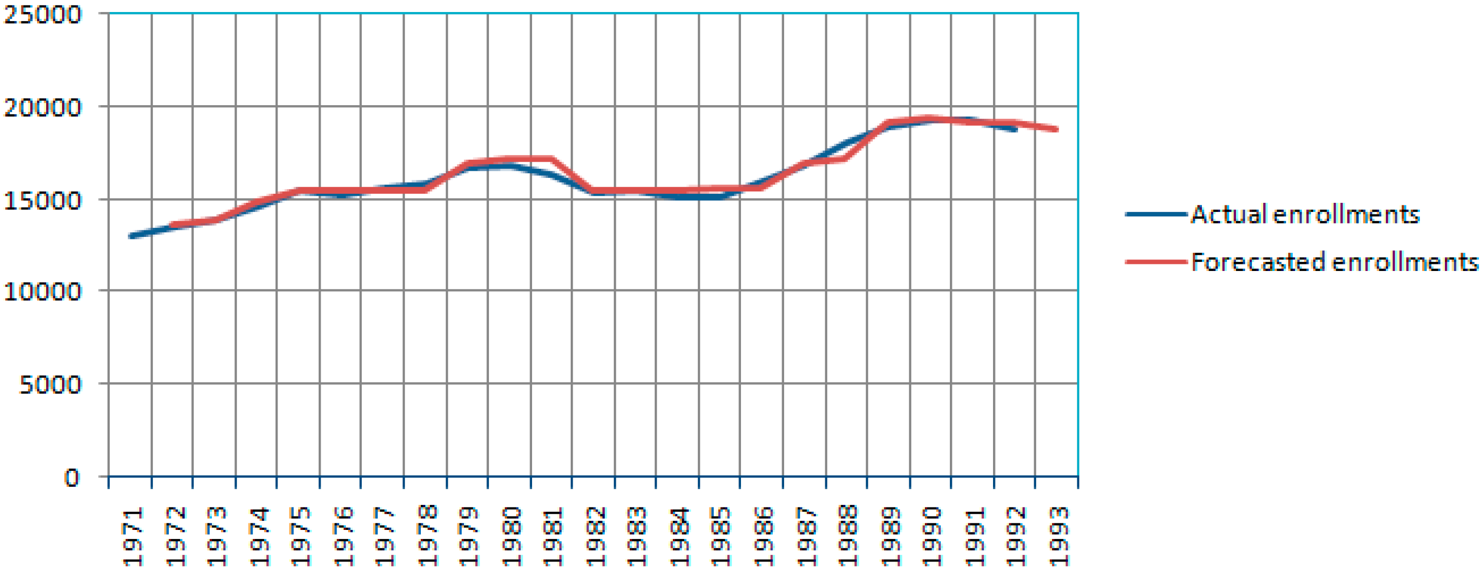
The other forecasted values are calculated in the same manner.
The actual and forecasted values of enrollments appear in Figure 1.
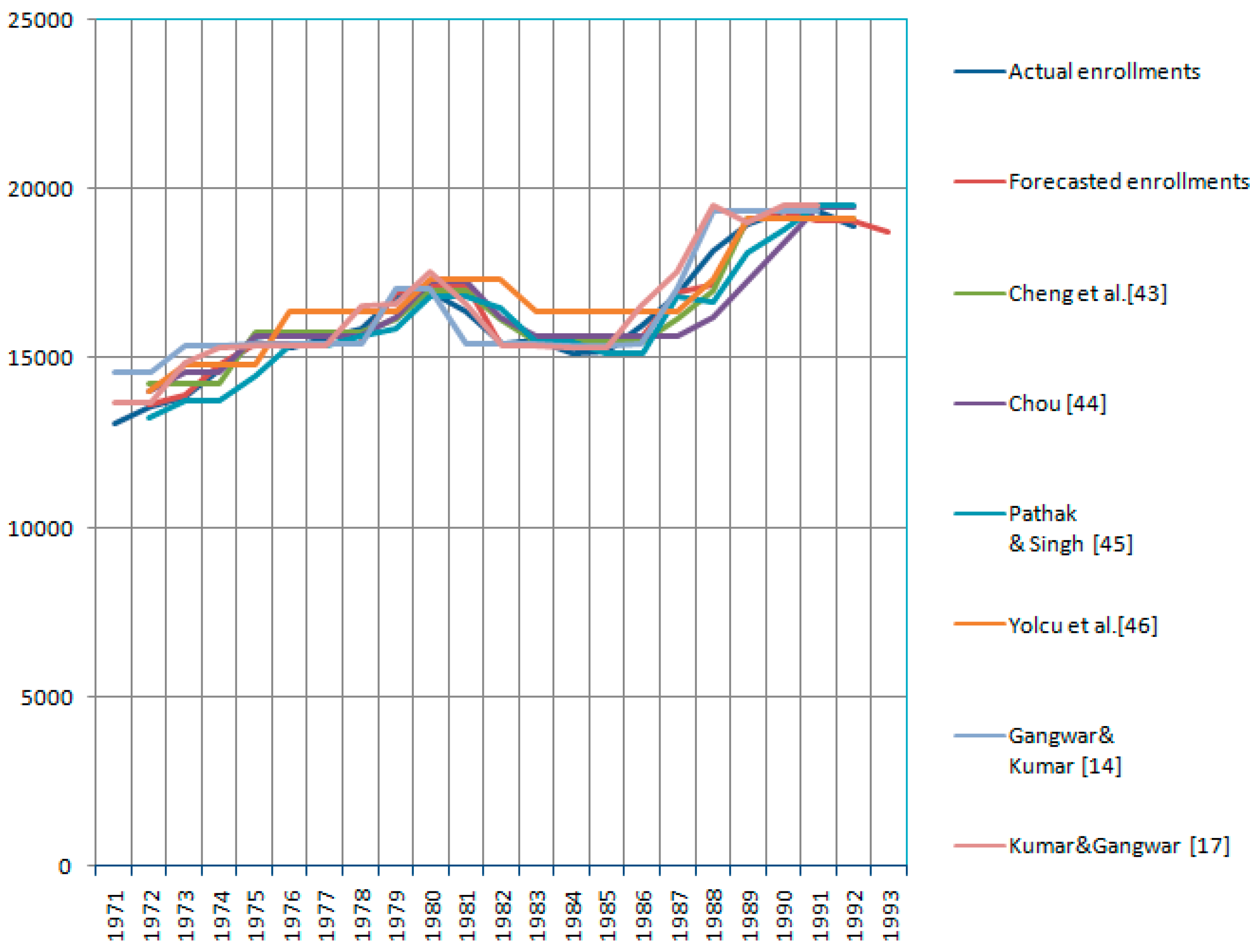
The forecasted enrollment data obtained with the suggested method, along with the forecasted data obtained with the models in [14,17,43,44,45,46], are presented in Table 5.
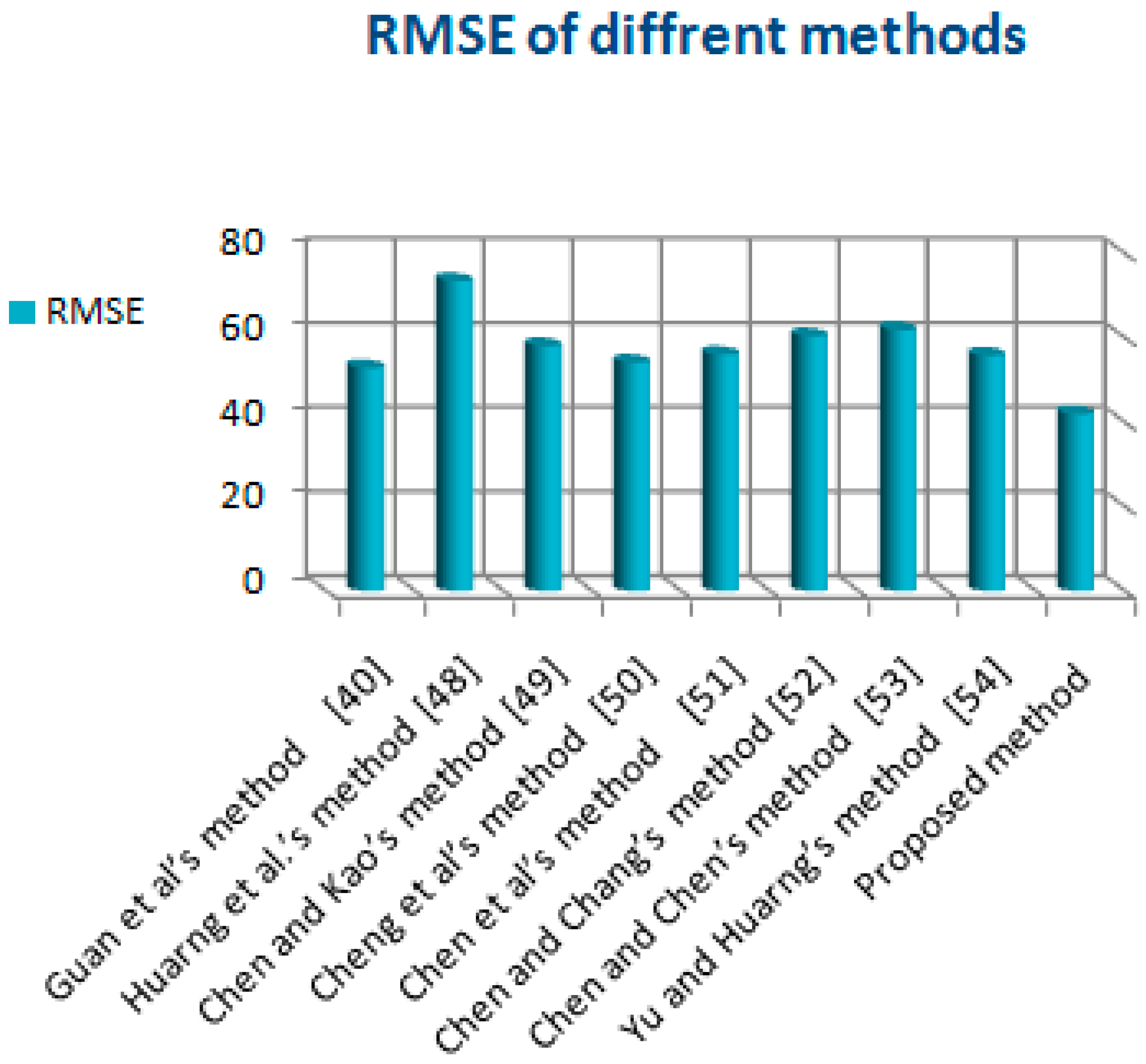
By comparing the proposed method with other existing methods in Table 5, the RMSE and AFE tools confirm that the suggested method is better than others, as shown in Table 6.
We combined forecasted values with respect to all methods in Figure 2.
If we plan to find the second-order neutrosophic logical relationships of the previous example by applying the proposed method of forecasting based on the second-order NTS, they are as shown in Table 7.
The second-order neutrosophic logical relationship groups of the previous example are as shown in Table 8.
We compared forecasted values of enrollments based on the second order of neutrosophic logical relationship groups of the proposed method with the method of second order presented by Gautam and Singh [47]. The results are shown in Table 9.
The MSE and AFE of the two methods are presented in Table 10.
From Table 10, it appears that our proposed method of second order is also better than the proposed method of second order presented by Gautam and Singh [47].
In addition, the third-order neutrosophic logical relationship groups of the previous example are constructed and shown in Table 11.
We also compared the forecasted values of enrollments based on the third order of neutrosophic logical relationship groups of the proposed method with the proposed methods of third order presented by [8,9,47], and the results are shown in Table 12.
The MSE and AFE of the methods are presented in Table 13.

4.2. Numerical Example 2

We verified the proposed method by solving the TAIEX2004 example [40], and by putting D 1 and D 2 equal 56 and 61 , respectively, then U = [ 5600.17 ,   6200.69 ]. Also we calculated the suitable length as we illustrated previously and found that it is equal to 40. Therefore, the number of triangular neutrosophic numbers is equal to 12. For these neutrosophic numbers, the decision makers determined the truth, indeterminacy, and falsity degrees equal to 0.9 , 0.1 , 0.1 , respectively. The actual and forecasted values of the TAIEX2004 example are presented in Table 14 and Figure 3.
The RMSE and AFE of the proposed method are presented in Table 15.
To confirm the performance of the suggested method, we compared it with other existing methods and the results are shown in Table 16 and Figure 4.
TAIEX2004 is used as a baseline to compare our method with other competitive methods, to compare and identify how all the methods can manage error reduction. The RMSE is a common approach used in financial analysis [55]. Compared with the existing methods as shown in Table 16, our proposed method can offer the least presence of errors since it has the most minimized RMSE. In other words, our method appears to be performing the best in reducing errors and ensuring all our analyses are accurate with insights. This may provide a new insight for business intelligence with artificial intelligence, cloud computing, and neutrosophic research.

5. Conclusion and Future Directions

The objective of this research was to enhance the accuracy rates of forecasting, since the forecasting accuracy rates in the existing approaches of fuzzy and intuitionistic fuzzy time series were not accurate enough. Thus, in this research we introduced the notion of first-and high-order neutrosophic time series data by defining the fitting length of intervals and proposing a novel method for calculating forecasted values. In order to obtain truth, indeterminacy, and falsity membership degrees of historical data, we defined triangular neutrosophic numbers. The neutrosophication process of historical time series data depends on the biggest score function of the triangular neutrosophic numbers. For the deneutrosophication process of first- and high-order NTS, we used simple arithmetic computations. The suggested approach of first- and high-order neutrosophic time series proved its superiority against other existing methods in the field of fuzzy, intuitionistic fuzzy, and neutrosophic time series. In the future, we plan to apply meta-heuristic optimization techniques for improving the accuracy of the suggested method. We will apply this model for predicting other time series, such as demand forecasting, electricity consumption, etc. Furthermore, we may consider using other approaches for comparing similarities of historical data, like information entropy.

Author Contributions

All authors contributed equally to this research. The individual responsibilities and contribution of all authors can be described as follows: the idea of this entire paper was put forward by M.A.-B. and M.M.; V.C. completed the preparatory work of the paper. F.S. analyzed the existing work. The revision and submission of this paper was completed by F.S. and M.A.-B.

Funding

This research received no external funding.

Acknowledgments

The authors are very thankful to the reviewers for their constructive suggestion to improve the quality of this research.

Conflicts of Interest

The authors declare no conflict of interest.

References

  1. Song, Q.; Chissom, B.S. Forecasting enrollments with fuzzy time series—Part I. Fuzzy Sets Syst. 1993, 54, 1–9. [Google Scholar] [CrossRef]
  2. Song, Q.; Chissom, B.S. Forecasting enrollments with fuzzy time series—Part II. Fuzzy Sets Syst. 1994, 62, 1–8. [Google Scholar] [CrossRef]
  3. Chen, S.M. Forecasting enrollments based on fuzzy time series. Fuzzy Sets Syst. 1996, 81, 311–319. [Google Scholar] [CrossRef]
  4. Lee, H.S.; Chou, M.T. Fuzzy forecasting based on fuzzy time series. Int. J. Comput. Math. 2004, 81, 781–789. [Google Scholar] [CrossRef]
  5. Singh, S.R. A simple method of forecasting based on fuzzy time series. Appl. Math. Comput. 2007, 186, 330–339. [Google Scholar] [CrossRef]
  6. Singh, S.R. A robust method of forecasting based on fuzzy time series. Appl. Math. Comput. 2007, 188, 472–484. [Google Scholar] [CrossRef]
  7. Tsaur, R.C.; Yang, J.C.O.; Wang, H.F. Fuzzy relation analysis in fuzzy time series model. Comput. Math. Appl. 2005, 49, 539–548. [Google Scholar] [CrossRef]
  8. Chen, S.M. Forecasting enrollments based on high-order fuzzy time series. Cybern. Syst. 2002, 33, 1–16. [Google Scholar] [CrossRef]
  9. Singh, S.R. A simple time variant method for fuzzy time series forecasting. Cybern. Syst. Int. J. 2007, 38, 305–321. [Google Scholar] [CrossRef]
  10. Hsu, Y.Y.; Tse, S.M.; Wu, B. A new approach of bivariate fuzzy time series analysis to the forecasting of a stock index. Int. J. Uncertain. Fuzziness Knowl.-Based Syst. 2003, 11, 671–690. [Google Scholar] [CrossRef]
  11. Ziemba, P.; Becker, J. Analysis of the Digital Divide Using Fuzzy Forecasting. Symmetry 2019, 11, 166. [Google Scholar] [CrossRef]
  12. Zadeh, L.A. On fuzzy algorithms. In Fuzzy Sets, Fuzzy Logic, and Fuzzy Systems: Selected Papers by Lotfi A Zadeh; World Scientific: Singapore, 1996; pp. 127–147. [Google Scholar]
  13. Atanassov, K.T. Intuitionistic fuzzy sets. Fuzzy Sets Syst. 1986, 20, 87–96. [Google Scholar] [CrossRef]
  14. Gangwar, S.S.; Kumar, S. Probabilistic and intuitionistic fuzzy sets—Based method for fuzzy time series forecasting. Cybern. Syst. 2014, 45, 349–361. [Google Scholar] [CrossRef]
  15. Wang, Y.N.; Lei, Y.; Fan, X.; Wang, Y. Intuitionistic fuzzy time series forecasting model based on intuitionistic fuzzy reasoning. Math. Prob. Eng. 2016, 2016, 5035160. [Google Scholar] [CrossRef]
  16. Joshi, B.P.; Kumar, S. Intuitionistic fuzzy sets based method for fuzzy time series forecasting. Cybern. Syst. 2012, 43, 34–47. [Google Scholar] [CrossRef]
  17. Kumar, S.; Gangwar, S.S. Intuitionistic fuzzy time series: An approach for handling non-determinism in time series forecasting. IEEE Trans. Fuzzy Syst. 2016, 24, 1270–1281. [Google Scholar] [CrossRef]
  18. Kumar, S.; Gangwar, S.S. A fuzzy time series forecasting method induced by intuitionistic fuzzy sets. Int. J. Model. Simul. Sci. Comput. 2015, 6, 1550041. [Google Scholar] [CrossRef]
  19. Eğrioglu, E.; Aladag, C.H.; Yolcu, U.; Dalar, A.Z. A hybrid high order fuzzy time series forecasting approach based on PSO and ANNS methods. Am. J. Intell. Syst. 2016, 6, 22–29. [Google Scholar]
  20. Cai, Q.; Zhang, D.; Wu, B.; Leung, S.C. A novel stock forecasting model based on fuzzy time series and genetic algorithm. Procedia Comput. Sci. 2013, 18, 1155–1162. [Google Scholar] [CrossRef]
  21. Huang, Y.L.; Horng, S.J.; He, M.; Fan, P.; Kao, T.W.; Khan, M.K.; Kuo, I.H. A hybrid forecasting model for enrollments based on aggregated fuzzy time series and particle swarm optimization. Expert Syst. Appl. 2011, 38, 8014–8023. [Google Scholar] [CrossRef]
  22. Bisht, K.; Kumar, S. Fuzzy time series forecasting method based on hesitant fuzzy sets. Expert Syst. Appl. 2016, 64, 557–568. [Google Scholar] [CrossRef]
  23. Bahrami, B.; Shafiee, M. Fuzzy descriptor models for earthquake time prediction using seismic time series. Int. J. Uncertain. Fuzziness Knowl.-Based Syst. 2015, 23, 505–519. [Google Scholar] [CrossRef]
  24. Wang, Y.; Lei, Y.; Wang, Y.; Zheng, K. A heuristic adaptive-order intuitionistic fuzzy time series forecasting model. J. Electron. Inf. Technol. 2016, 38, 2795–2802. [Google Scholar]
  25. Abhishekh, S.S.G.; Singh, S.R. A refined weighted method for forecasting based on type 2 fuzzy time series. Int. J. Model. Simul. 2018, 38, 180–188. [Google Scholar] [CrossRef]
  26. Abhishekh, S.S.G.; Singh, S.R. A score function-based method of forecasting using intuitionistic fuzzy time series. New Math. Nat. Comput. 2018, 14, 91–111. [Google Scholar] [CrossRef]
  27. Abhishekh, S.K. A computational method for rice production forecasting based on high-order fuzzy time series. Int. J. Fuzzy Math. Arch. 2017, 13, 145–157. [Google Scholar]
  28. Abdel-Basset, M.; Mohamed, M.; Chang, V. NMCDA: A framework for evaluating cloud computing services. Future Gener. Comput. Syst. 2018, 86, 12–29. [Google Scholar] [CrossRef]
  29. Smarandache, F. A Unifying Field in Logics: Neutrosophic Logic. In Neutrosophy, Neutrosophic Set, Neutrosophic Probability, 3rd ed.; American Research Press: Rehoboth, DE, USA, 1999; Volume 8, pp. 489–503. [Google Scholar]
  30. Abdel-Basset, M.; Mohamed, M. The role of single valued neutrosophic sets and rough sets in smart city: Imperfect and incomplete information systems. Measurement 2018, 124, 47–55. [Google Scholar] [CrossRef]
  31. Abdel-Basset, M.; Mohamed, M.; Smarandache, F.; Chang, V. Neutrosophic Association Rule Mining Algorithm for Big Data Analysis. Symmetry 2018, 10, 106. [Google Scholar] [CrossRef]
  32. Abdel-Basset, M.; Mohamed, M.; Zhou, Y.; Hezam, I. Multi-criteria group decision making based on neutrosophic analytic hierarchy process. J. Intell. Fuzzy Syst. 2017, 33, 4055–4066. [Google Scholar] [CrossRef]
  33. Abdel-Basset, M.; Gunasekaran, M.; Mohamed, M.; Smarandache, F. A novel method for solving the fully neutrosophic linear programming problems. Neural Comput. Appl. 2018, 1–11. [Google Scholar] [CrossRef]
  34. Abdel-Basset, M.; Mohamed, M.; Sangaiah, A.K. Neutrosophic AHP-Delphi Group decision making model based on trapezoidal neutrosophic numbers. J. Ambient Intell. Hum. Comput. 2018, 9, 1427–1443. [Google Scholar] [CrossRef]
  35. Abdel-Basset, M.; Mohamed, M.; Hussien, A.N.; Sangaiah, A.K. A novel group decision-making model based on triangular neutrosophic numbers. Soft Comput. 2018, 22, 6629–6643. [Google Scholar] [CrossRef]
  36. Abdel-Basset, M.; Zhou, Y.; Mohamed, M.; Chang, V. A group decision making framework based on neutrosophic VIKOR approach for e-government website evaluation. J. Intell. Fuzzy Syst. 2018, 34, 4213–4224. [Google Scholar] [CrossRef]
  37. Abdel-Basset, M.; Gunasekaran, M.; Mohamed, M.; Chilamkurti, N. Three-way decisions based on neutrosophic sets and AHP-QFD framework for supplier selection problem. Futur. Gener. Comput. Syst. 2018, 89, 19–30. [Google Scholar] [CrossRef]
  38. Mohamed, M.; Abdel-Baset, M.; Smarandache, F.; Zhou, Y. A Critical Path Problem in Neutrosophic Environment; Infinite Study: El Segundo, CA, USA, 2017. [Google Scholar]
  39. Abdel-Basset, M.; Mohamed, M.; Smarandache, F. A hybrid neutrosophic group ANP-TOPSIS framework for supplier selection problems. Symmetry 2018, 10, 226. [Google Scholar] [CrossRef]
  40. Guan, H.; He, J.; Zhao, A.; Dai, Z.; Guan, S. A Forecasting Model Based on Multi-Valued Neutrosophic Sets and Two-Factor, Third-Order Fuzzy Fluctuation Logical Relationships. Symmetry 2018, 10, 245. [Google Scholar] [CrossRef]
  41. Guan, H.; Dai, Z.; Guan, S.; Zhao, A. A Forecasting Model Based on High-Order Fluctuation Trends and Information Entropy. Entropy 2018, 20, 669. [Google Scholar] [CrossRef]
  42. Huarng, K. Effective lengths of intervals to improve forecasting in fuzzy time series. Fuzzy Sets Syst. 2001, 123, 387–394. [Google Scholar] [CrossRef]
  43. Cheng, C.H.; Cheng, G.W.; Wang, J.W. Multi-attribute fuzzy time series method based on fuzzy clustering. Expert Syst. Appl. 2008, 34, 1235–1242. [Google Scholar] [CrossRef]
  44. Chou, M.T. Long-term predictive value interval with the fuzzy time series. J. Mar. Sci. Technol. 2011, 19, 509–513. [Google Scholar]
  45. Pathak, H.K.; Singh, P. A new bandwidth interval based forecasting method for enrollments using fuzzy time series. Appl. Math. 2011, 2, 504–507. [Google Scholar] [CrossRef]
  46. Yolcu, U.; Egrioglu, E.; Uslu, V.R.; Basaran, M.A.; Aladag, C.H. A new approach for determining the length of intervals for fuzzy time series. Appl. Soft Comput. 2009, 9, 647–651. [Google Scholar] [CrossRef]
  47. Gautam, S.S.; Singh, S.R. A refined method of forecasting based on high-order intuitionistic fuzzy time series data. Prog. Artif. Intell. 2018, 7, 339–350. [Google Scholar]
  48. Huarng, K.H.; Yu, T.H.K.; Hsu, Y.W. A multivariate heuristic model for fuzzy time-series forecasting. IEEE Trans. Syst. Man Cybern. Part B (Cybern.) 2007, 37, 836–846. [Google Scholar] [CrossRef]
  49. Chen, S.M.; Kao, P.Y. TAIEX forecasting based on fuzzy time series, particle swarm optimization techniques and support vector machines. Inf. Sci. 2013, 247, 62–71. [Google Scholar] [CrossRef]
  50. Cheng, S.H.; Chen, S.M.; Jian, W.S. Fuzzy time series forecasting based on fuzzy logical relationships and similarity measures. Inf. Sci. 2016, 327, 272–287. [Google Scholar] [CrossRef]
  51. Chen, S.M.; Manalu, G.M.T.; Pan, J.S.; Liu, H.C. Fuzzy forecasting based on two-factors second-order fuzzy-trend logical relationship groups and particle swarm optimization techniques. IEEE Trans. Cybern. 2013, 43, 1102–1117. [Google Scholar] [CrossRef] [PubMed]
  52. Chen, S.M.; Chang, Y.C. Multi-variable fuzzy forecasting based on fuzzy clustering and fuzzy rule interpolation techniques. Inf. Sci. 2010, 180, 4772–4783. [Google Scholar] [CrossRef]
  53. Chen, S.M.; Chen, C.D. TAIEX forecasting based on fuzzy time series and fuzzy variation groups. IEEE Trans. Fuzzy Syst. 2011, 19, 1–12. [Google Scholar] [CrossRef]
  54. Yu, T.H.K.; Huarng, K.H. A neural network-based fuzzy time series model to improve forecasting. Expert Syst. Appl. 2010, 37, 3366–3372. [Google Scholar] [CrossRef]
  55. Chang, V. The business intelligence as a service in the cloud. Futur. Gener. Comput. Syst. 2014, 37, 512–534. [Google Scholar] [CrossRef]
Figure 1. Forecasted and actual enrollments.
Symmetry 11 00457 g001
Figure 2. Comparison figures between all forecasted values.
Symmetry 11 00457 g002
Figure 3. Actual and forecasted values of TAIEX2004.
Symmetry 11 00457 g003
Figure 4. The RMSE of different methods that solved the TAIEX2004 example.
Symmetry 11 00457 g004
Table 1. Actual and neutrosophication values of student enrollments.
YearsActual Enrollments Neutrosophication   Values   of   Enrollments   N ˜
197113,055 N ˜ 1
197213,563 N ˜ 2
197313,867 N ˜ 3
197414,696 N ˜ 6
197515,460 N ˜ 8
197615,311 N ˜ 8
197715,603 N ˜ 8
197815,861 N ˜ 9
197916,807 N ˜ 13
198016,919 N ˜ 13
198116,388 N ˜ 11
198215,433 N ˜ 8
198315,497 N ˜ 8
198415,145 N ˜ 7
198515,163 N ˜ 7
198615,984 N ˜ 10
198716,859 N ˜ 13
198818,150 N ˜ 17
198918,970 N ˜ 20
199019,328 N ˜ 21
199119,337 N ˜ 21
199218,876 N ˜ 19
Table 2. Neutrosophic logical relationships.
N ˜ 1 N ˜ 2 N ˜ 2 N ˜ 3 N ˜ 3 N ˜ 6 N ˜ 6 N ˜ 8 N ˜ 8 N ˜ 8
N ˜ 8 N ˜ 9 N ˜ 9 N ˜ 13 N ˜ 13 N ˜ 13 N ˜ 13 N ˜ 11 N ˜ 11 N ˜ 8
N ˜ 8 N ˜ 7 N ˜ 7 N ˜ 7 N ˜ 7 N ˜ 10 N ˜ 10 N ˜ 13 N ˜ 13 N ˜ 17
N ˜ 17 N ˜ 20 N ˜ 20 N ˜ 21 N ˜ 21 N ˜ 21 N ˜ 21 N ˜ 19
Table 3. Neutrosophic logical relationship groups (NLRGs) of enrollments.
N ˜ 1 N ˜ 2
N ˜ 2 N ˜ 3
N ˜ 3 N ˜ 6
N ˜ 6 N ˜ 8
N ˜ 7 N ˜ 7 N ˜ 7 N ˜ 10
N ˜ 8 N ˜ 7 N ˜ 8 N ˜ 8 N ˜ 8 N ˜ 9
N ˜ 9 N ˜ 13
N ˜ 10 N ˜ 13
N ˜ 11 N ˜ 8
N ˜ 13 N ˜ 11 N ˜ 13 N ˜ 13 N ˜ 13 N ˜ 17
N ˜ 17 N ˜ 20
N ˜ 20 N ˜ 21
N ˜ 21 N ˜ 19 N ˜ 21 N ˜ 21
Table 4. Actual and forecasted values of enrollments.
YearsActual EnrollmentsForecasted Values of Enrollments
197113,055
197213,563 13,650
197313,86713,950
197414,696 14,850
197515,460 15,450
197615,311 15,450
197715,603 15,450
197815,861 15,450
197916,807 16,950
198016,919 17,150
198116,388 17,150
198215,43315,450
198315,497 15,450
198415,145 15,450
198515,163 15,600
198615,984 15,600
198716,859 16,950
198818,150 17,150
198918,970 19,050
199019,328 19,350
199119,337 19,050
199218,876 19,050
Table 5. Forecasted values by suggested method and other methods.
YearsActual ValuesForecasted Values
Proposed[43][44][45][46][14][17]
197113,055
197213,563 13 , 650 14,242.014,02513,25014,031.3514,58613,693
197313,86713,95014,242.014,56813,75014,795.3614,58613,693
197414,696 14 , 850 14,242.014,56813,75014,795.3615,36314,867
197515,460 15 , 450 15,774.315,65414,50014,795.3615,36315,287
197615,311 15 , 450 15,774.315,65415,37516,406.5715,44215,376
197715,603 15 , 450 15,774.315,65415,37516,406.5715,44215,376
197815,861 15 , 450 15,774.315,65415,62516,406.5715,44215,376
197916,807 16 , 950 16,146.516,19715,87516,406.5715,44216,523
198016,919 17 , 150 16,988.317,28316,83317,315.2917,06416,606
198116,388 17 , 150 16,988.317,28316,83317,315.2917,06417,519
198215,433 15 , 450 16,146.516,19716,50017,315.2915,43816,606
198315,497 15 , 450 15,474.315,65415,50016,406.5715,44215,376
198415,145 15 , 450 15,474.315,65415,50016,406.5715,44215,376
198515,163 15 , 600 15,474.315,65415,12516,406.5715,36315,287
198615,984 15 , 600 15,474.315,65415,12516,406.5715,36315,287
198716,859 16 , 950 16,146.515,65416,83316,406.5715,43816,523
198818,150 17 , 150 16,988.316,19716,66717,315.2917,06417,519
198918,970 19 , 050 19,144.017,28318,12519,132.7919,35619,500
199019,328 19 , 350 19,144.018,36918,75019,132.7919,35619,000
199119,337 19 , 050 19,144.019,45419,50019,132.7919,35619,500
199218,876 19 , 050 19,144.019,45419,50019,132.7919,35619,500
Table 6. Error measures.
ToolProposed[43][44][45][46][14][17]
RMSE342.68478.45781.47646.67805.17642.68493.56
AFE (%)1.442.393.612.984.282.962.33
Table 7. Second-order NLR.
N ˜ 1 , N ˜ 2 N ˜ 3
N ˜ 2 , N ˜ 3 N ˜ 6
N ˜ 3 , N ˜ 6 N ˜ 8
N ˜ 6 , N ˜ 8 N ˜ 8
N ˜ 8 , N ˜ 8 N ˜ 8
N ˜ 8 , N ˜ 8 N ˜ 9
N ˜ 8 , N ˜ 9 N ˜ 13
N ˜ 9 , N ˜ 13 N ˜ 13
N ˜ 13 , N ˜ 13 N ˜ 11 N ˜ 13 , N ˜ 11 N ˜ 8
N ˜ 11 , N ˜ 8 N ˜ 8
N ˜ 8 , N ˜ 8 N ˜ 7
N ˜ 8 , N ˜ 7 N ˜ 7
N ˜ 7 , N ˜ 7 N ˜ 10
N ˜ 7 , N ˜ 10 N ˜ 13
N ˜ 10 , N ˜ 13 N ˜ 17
N ˜ 13 , N ˜ 17 N ˜ 20
N ˜ 17 , N ˜ 20 N ˜ 21
N ˜ 20 , N ˜ 21 N ˜ 21
N ˜ 21 , N ˜ 21 N ˜ 19
Table 8. Second-order NLRGs.
N ˜ 1 , N ˜ 2 N ˜ 3
N ˜ 2 , N ˜ 3 N ˜ 6
N ˜ 3 , N ˜ 6 N ˜ 8
N ˜ 6 , N ˜ 8 N ˜ 8
N ˜ 8 , N ˜ 8 N ˜ 8 N ˜ 8 , N ˜ 8 N ˜ 9 N ˜ 8 , N ˜ 8 N ˜ 7
N ˜ 8 , N ˜ 9 N ˜ 13
N ˜ 9 , N ˜ 13 N ˜ 13
N ˜ 13 , N ˜ 13 N ˜ 11
N ˜ 13 , N ˜ 11 N ˜ 8
N ˜ 11 , N ˜ 8 N ˜ 8
N ˜ 8 , N ˜ 7 N ˜ 7
N ˜ 7 , N ˜ 7 N ˜ 10
N ˜ 7 , N ˜ 10 N ˜ 13
N ˜ 10 , N ˜ 13 N ˜ 17
N ˜ 13 , N ˜ 17 N ˜ 20
N ˜ 17 , N ˜ 20 N ˜ 21
N ˜ 20 , N ˜ 21 N ˜ 21
N ˜ 21 , N ˜ 21 N ˜ 19
Table 9. Actual and forecasted values of enrollments based on the second order of the proposed method vs. the Gautam and Singh [47] method.
YearsActual EnrollmentsSecond-Order Forecasted Values of the Proposed MethodForecasted Values in [47]
197113,055
197213,563
197313,86713,95013,800
197414,696 14 , 850 14,400
197515,460 15 , 450 15,300
197615,311 15 , 450 15,300
197715,603 15 , 450 15,600
197815,861 15 , 450 15,600
197916,807 16 , 950 16,800
198016,919 16 , 950 16,800
198116,388 16 , 350 16,200
198215,433 15 , 450 15,300
198315,497 15 , 450 15,300
198415,14515,45015,000
198515,163 15 , 150 15,000
198615,984 16 , 050 15,900
198716,859 16 , 950 16,800
198818,150 18 , 150 18,000
198918,970 19 , 050 18,900
199019,328 19 , 350 19,200
199119,337 19 , 350 19,200
199218,876 18 , 750 18,600
Table 10. Error measures of the proposed method and the Gautam and Singh method [47].
ToolProposed[47]
MSE19,823.424,443.4
AFE (%)0.600.81
Table 11. Third-order NLRGs.
N ˜ 1 , N ˜ 2 , N ˜ 3 N ˜ 6
N ˜ 2 , N ˜ 3 , N ˜ 6 N ˜ 8
N ˜ 3 , N ˜ 6 , N ˜ 8 N ˜ 8
N ˜ 6 , N ˜ 8 , N ˜ 8 N ˜ 8
N ˜ 8 , N ˜ 8 , N ˜ 8 N ˜ 9
N ˜ 8 , N ˜ 8 , N ˜ 9 N ˜ 13
N ˜ 8 , N ˜ 9 , N ˜ 13 N ˜ 13
N ˜ 9 , N ˜ 13 , N ˜ 13 N ˜ 11
N ˜ 13 , N ˜ 13 , N ˜ 11 N ˜ 8
N ˜ 13 , N ˜ 11 , N ˜ 8 N ˜ 8
N ˜ 11 , N ˜ 8 , N ˜ 8 N ˜ 7
N ˜ 8 , N ˜ 8 , N ˜ 7 N ˜ 7
N ˜ 8 , N ˜ 7 , N ˜ 7 N ˜ 10
N ˜ 7 , N ˜ 7 , N ˜ 10 N ˜ 13
N ˜ 7 , N ˜ 10 , N ˜ 13 N ˜ 17
N ˜ 10 , N ˜ 13 , N ˜ 17 N ˜ 20
N ˜ 13 , N ˜ 17 , N ˜ 20 N ˜ 21
N ˜ 17 , N ˜ 20 , N ˜ 21 N ˜ 21
N ˜ 20 , N ˜ 21 , N ˜ 21 N ˜ 19
Table 12. Actual and forecasted values of enrollments based on the third order of the proposed method vs. the methods presented by [8,9,47].
YearsActual EnrollmentsThird-Order Forecasted Values of the Proposed MethodForecasted Values in [47]Forecasted Values in [8]Forecasted Values in [9]
197113,055
197213,563
197313,867
197414,69614,85014,40014,50014,750
197515,46015,45015,30015,50015,750
197615,31115,45015,30015,50015,500
197715,60315,45015,60015,50015,500
197815,86115,75015,60015,50015,500
197916,80716,95016,80016,50016,500
198016,91916,95016,80016,50016,500
198116,38816,35016,20016,50016,500
198215,43315,45015,30015,50015,500
198315,49715,45015,30015,50015,500
198415,14515,15015,00015,50015,250
198515,16315,15015,00015,50015,500
198615,98416,05015,90015,50015,500
198716,85916,95016,80016,50016,500
198818,15018,15018,00018,50018,500
198918,97019,05018,90018,50018,500
199019,32819,35019,20019,50019,500
199119,33719,35019,20019,50019,500
199218,87618,75018,60018,50018,750
Table 13. Error measures of the proposed method and the [8,9,47] methods.
ToolProposed[47][8][9]
MSE7367.31625,493.686,69476,509
AFE (%)0.400.821.521.40
Table 14. Actual and forecasted values of TAIEX2004.
DatesActual ValuesForecasted Values of the Proposed Method
01/11/20045656.17
02/11/20045759.615760.17
03/11/20045862.855813.5
04/11/20045860.735900.17
05/11/20045931.315900.17
08/11/20045937.465903.02
09/11/20045945.25903.02
10/11/20045948.495940.17
11/11/20045874.525940.17
12/11/20045917.165903.02
15/11/20045906.695903.02
16/11/20045910.855903.02
17/11/20046028.685940.17
18/11/20046049.495940.17
19/11/20046026.555940.17
22/11/20045838.425830.17
23/11/20045851.15830.17
24/11/20045911.315903.02
25/11/20045855.245830.17
26/11/20045778.655813.5
29/11/20045785.265813.5
30/11/20045844.765860.17
1/12/20045798.625830.17
02/12/20045867.955860.17
03/12/20045893.275900.17
06/12/20045919.175900.17
07/12/20045925.285903.02
08/12/20045892.515903.02
09/12/20045913.975900.17
10/12/20045911.635903.02
13/12/20045878.895903.02
14/12/20045909.655900.17
15/12/20046002.585903.02
16/12/20046019.236040.17
17/12/20046009.326040.17
20/12/20045985.946040.17
21/12/20045987.856040.17
22/12/20046001.526040.17
23/12/20045997.676040.17
24/12/20046019.426040.17
27/12/20045985.946040.17
28/12/20046000.576040.17
29/12/20046088.496040.17
30/12/20046100.866080.17
31/12/20046139.696080.17
Table 15. Error measures of the proposed method.
ToolProposed
RMSE42.05
AFE (%)0.005
Table 16. Error measures of the proposed method and other existing methods which solved the TAIEX2004 example.
MethodsRMSE
Guan et al.’s method [40]53.01
Huarng et al.’s method [48]73.57
Chen and Kao’s method [49]58.17
Cheng et al.’s method [50]54.24
Chen et al.’s method [51]56.16
Chen and Chang’s method [52]60.48
Chen and Chen’s method [53]61.94
Yu and Huarng’s method [54]55.91
Proposed method42.05

