Scale Invariant Effective Hamiltonians for a Graph with a Small Compact Core

Abstract

We consider a compact metric graph of size $\epsilon$ and attach to it several edges (leads) of length of order one (or of infinite length). As $\epsilon$ goes to zero, the graph ${\mathcal{G}}^{\epsilon }$ obtained in this way looks like the star-graph formed by the leads joined in a central vertex. On ${\mathcal{G}}^{\epsilon }$ we define an Hamiltonian $H^{\epsilon }$, properly scaled with the parameter $\epsilon$. We prove that there exists a scale invariant effective Hamiltonian on the star-graph that approximates $H^{\epsilon }$ (in a suitable norm resolvent sense) as $\epsilon \to 0$. The effective Hamiltonian depends on the spectral properties of an auxiliary $\epsilon$-independent Hamiltonian defined on the compact graph obtained by setting $\epsilon =1$. If zero is not an eigenvalue of the auxiliary Hamiltonian, in the limit $\epsilon \to 0$, the leads are decoupled.

1. Introduction

One nice feature of quantum graphs (metric graphs equipped with differential operators) is that they are simple objects. In many cases, for example in the framework of the analysis of self-adjoint realizations of the Laplacian, it is possible to write down explicit formulae for the relevant quantities, such as the resolvent or the scattering matrix (see, e.g., [1] and [2]).

If the graph is too intricate though, it can be difficult, if not impossible, to perform exact computations. In such a situation, one may be interested in a simpler, effective model which captures only the most essential features of a complex quantum graph.

If several edges of the graph are much shorter then others, an effective model should rely on a simpler graph obtained by shrinking the short edges into vertices. These new vertices should keep track of at least some of the spectral or scattering properties of the shrinking edges, and perform as a black box approximation for a small, possibly intricate, network.

Our goal is to understand under what circumstances this type of effective models can be implemented. In this report we give some preliminary results showing that under certain assumptions such approximation is possible.

To fix the ideas, consider a compact metric graph ${\mathcal{G}}^{in,\epsilon }$ of size (total length) $\epsilon$, and attach to it several edges of length of order one (or of infinite length), the leads. Clearly, when $\epsilon$ goes to zero, the graph obtained in this way (let us denote it by ${\mathcal{G}}^{\epsilon }$) looks like the star-graph formed by the leads joined in a central vertex. Let us denote by ${\mathcal{G}}^{out}$ such star-graph and by $v_0$ the central vertex.

Given a certain Hamiltonian (self-adjoint Schrödinger operator) $H^{\epsilon }$ on ${\mathcal{G}}^{\epsilon }$, we want to show that there exists an Hamiltonian $H^{out}$ on ${\mathcal{G}}^{out}$ such that, for small $\epsilon$, $H^{out}$ approximates (in a sense to be specified) $H^{\epsilon }$. Of course, one main issue is to understand what boundary conditions in the vertex $v_0$ characterize the domain of $H^{out}$.

It turns out that, under several technical assumptions, the boundary conditions in $v_0$ are fully determined by the spectral properties of an auxiliary, $\epsilon$-independent Hamiltonian defined on the graph ${\mathcal{G}}^{in}={\mathcal{G}}^{in,\epsilon =1}$.

Below we briefly discuss these technical assumptions, and refer to Section 2 for the details.

(i)

The Hamiltonian $H^{\epsilon }$ on ${\mathcal{G}}^{\epsilon }$ is a self-adjoint realization of the operator $-\Delta +B^{\epsilon }$ on ${\mathcal{G}}^{\epsilon }$, where $B^{\epsilon }$ is a potential term.

(ii)

To set up the graph ${\mathcal{G}}^{\epsilon }$ we select N distinct vertices in ${\mathcal{G}}^{in,\epsilon }$ (we call them connecting vertices) and attach to each of them one lead, which is either a finite or an infinite length edge. The domain of $H^{\epsilon }$ is characterized by Kirchhoff (also called standard or free) boundary conditions at the connecting vertices, i.e., in each connecting vertex functions are continuous and the sum of the outgoing derivatives equals zero.

(iii)

Scale invariance; the small (or inner) part of the graph scales uniformly in $\epsilon$, i.e., ${\mathcal{G}}^{in,\epsilon }=\epsilon {\mathcal{G}}^{in}$. The Hamiltonian $H^{\epsilon }$ has a specific scaling property with respect to the parameter $\epsilon$; loosely speaking, up to a multiplicative factor, the “restriction” of $H^{\epsilon }$ to ${\mathcal{G}}^{in,\epsilon }$ is unitarily equivalent to an $\epsilon$-independent operator on ${\mathcal{G}}^{in}$. The scale invariance property can be made precise by reasoning in terms of Hamiltonians on the inner graph ${\mathcal{G}}^{in,\epsilon }$. This is done in Section 4 below. Here we just mention that this assumption forces the scaling on the $in$ component of the potential $B^{in,\epsilon }(x)={\epsilon }^{-2}{B}^{in}(x/\epsilon )$, $x\in {\mathcal{G}}^{in,\epsilon }$, and, in the vertices of ${\mathcal{G}}^{in,\epsilon }$, the Robin-type vertex conditions (if any) also scale with $\epsilon$ accordingly.

(iv)

The “restriction” of $H^{\epsilon }$ to the leads does not depend on $\epsilon$. In particular, $B^{out}$, the $out$ component of the potential, does not depend on $\epsilon$.

We prove that it is always possible to identify an Hamiltonian $H^{out}$ on ${\mathcal{G}}^{out}$ that approximates the Hamiltonian $H^{\epsilon }$. The Hamiltonian $H^{out}$ is a self-adjoint realization of the operator $-\Delta +B^{out}$ on ${\mathcal{G}}^{out}$, and it is characterized by scale invariant vertex conditions in $v_0$, i.e., vertex conditions with no Robin part (see [3], Section 1.4.2); in our notation, scale invariant means ${\Theta }_v=0$ in Equation (1). The precise form of the possible effective Hamiltonians is given in Definitions 6 and 7 below.

The convergence of $H^{\epsilon }$ to $H^{out}$ is understood in the following sense. We look at the resolvent operator $R_z^{\epsilon }:={(H^{\epsilon }-z)}^{-1}$, $z\in \mathbb{C}\setminus \mathbb{R}$, as an operator in the Hilbert space $L^2({\mathcal{G}}^{\epsilon })=L^2({\mathcal{G}}^{out})\oplus L^2({\mathcal{G}}^{in,\epsilon })$. In the limit $\epsilon \to 0$, the bounded operator $R_z^{\epsilon }$ converges to an operator which is diagonal in the decomposition $L^2({\mathcal{G}}^{out})\oplus L^2({\mathcal{G}}^{in,\epsilon })$. The $out/out$ component of the limiting operator is the resolvent of a self-adjoint operator in $L^2({\mathcal{G}}^{out})$, which we identify as the effective Hamiltonian on the star-graph.

Additionally, we characterize the limiting boundary conditions in the vertex $v_0$ in terms of the spectral properties of an auxiliary Hamiltonian on the (compact) graph ${\mathcal{G}}^{in}={\mathcal{G}}^{in,\epsilon =1}$. We distinguish two mutually exclusive cases: in one case (that we call generic) zero is not an eigenvalue of the auxiliary Hamiltonian; in the other case (we call it non-generic) zero is an eigenvalue of the auxiliary Hamiltonian.

In the generic case the effective Hamiltonian, denoted by ${\mathring{H}}^{out}$, is characterized by Dirichlet (also called decoupling) boundary conditions in the vertex $v_0$, i.e., functions in its domain are zero in $v_0$, see Definition 6. From the point of view of applications this is the less interesting case, since the leads are decoupled (no transmission through $v_0$ is possible).

In the non-generic case the situation is more involved. If zero is an eigenvalue of the auxiliary Hamiltonian one can identify a corresponding set of orthonormal eigenfunctions (in general eigenvalues can have multiplicity larger than one, included the zero eigenvalue). In the domain of the effective Hamiltonian ${\widehat{H}}^{out}$, the boundary conditions in $v_0$ are associated to the values of these eigenfunctions in the connecting vertices, see Definition 7. In this case, the boundary conditions in the vertex $v_0$ are scale invariant but, in general, not of decoupling type. For example, if the multiplicity of the zero eigenvalue is one, and the corresponding eigenfunction assumes the same value in all the connecting vertices, the boundary conditions are of Kirchhoff type.

The proof of the convergence is based on a Kreĭn-type formula for the resolvent $R_z^{\epsilon }$. This formula allows us to write $R_z^{\epsilon }$ as a block matrix operator in the decomposition $L^2({\mathcal{G}}^{\epsilon })=L^2({\mathcal{G}}^{out})\oplus L^2({\mathcal{G}}^{in,\epsilon })$ (see Equation (31)). In the formula, the first term, ${\mathring{R}}_z^{\epsilon }$, is block diagonal and contains the resolvents of ${\mathring{H}}^{out}$ and ${\mathring{H}}^{in,\epsilon }$ (a scaled down version of the auxiliary Hamiltonian, see Section 2.4); the second term is non-trivial, and couples the $out$ and $in$ components to reconstruct the resolvent of the full Hamiltonian $H^{\epsilon }$. As $\epsilon$ goes to zero, the off-diagonal components in $R_z^{\epsilon }$ converge to zero, hence, the $out$ and $in$ components are always decoupled in the limit. A careful analysis of the non-trivial term in Formula (31) shows that it converges to zero in the generic case. In the non-generic case, instead, the $out/out$ component of the non-trivial term converges to a finite operator, and the whole $out/out$ component of $R_z^{\epsilon }$ reconstructs the resolvent of the effective Hamiltonian ${\widehat{H}}_0$.

The limiting behavior of $H^{\epsilon }$ is essentially determined by the small $\epsilon$ asymptotics of the spectrum of the inner Hamiltonian ${\mathring{H}}^{in,\epsilon }$. The scale invariance assumption implies that the eigenvalues of ${\mathring{H}}^{in,\epsilon }$ are given by ${\lambda }_n^{\epsilon }={\lambda }_n/{\epsilon }^2$, where ${\lambda }_n$ are the eigenvalues of the (scaled up) auxiliary Hamiltonian ${\mathring{H}}^{in}$. Obviously, all the non-zero eigenvalues move to infinity as $\epsilon \to 0$; the zero eigenvalue instead, if it exists, persists, and for this reason it plays a special role in the analysis.

Closely related to our work is the paper by G. Berkolaiko, Y. Latushkin, and S. Sukhtaiev [4], to which we refer also for additional references. In [4] the authors analyze the convergence of Schrödinger operators on metric graphs with shrinking edges. Our setting is similar to the one in [4] with several differences. In [4] there are no restrictions on the topology of the graph, i.e., ${\mathcal{G}}^{out}$ is not necessarily a star-graph; outer edges can form loops, be connected among them or to arbitrarily intricate finite length graphs. In [4], moreover, the scale invariance assumption is missing. With respect to our work, however, the potential terms in [4] do not play an essential role in the limiting problem (because they are uniformly bounded in the scaling parameter).

As it was done in [4], to analyze the convergence of $H^{\epsilon }$ to $H^{out}$, since they are operators on different Hilbert spaces, one could use the notion of ${\delta }^{\epsilon }$-quasi unitary equivalence (or generalized norm resolvent convergence) introduced by P. Exner and O. Post in the series of works [5,6,7,8,9]. In Theorems 1 and 2 we state our main results in terms of the expansion of the resolvent in the decomposition $L^2({\mathcal{G}}^{\epsilon })=L^2({\mathcal{G}}^{out})\oplus L^2({\mathcal{G}}^{in,\epsilon })$; and comment on the ${\delta }^{\epsilon }$-quasi unitary equivalence of the operators $H^{\epsilon }$ and ${\mathring{H}}^{out}$ (or ${\widehat{H}}^{out}$) in Remark 6.

Our analysis, with the scaling on the potential $B^{in,\epsilon }(x)={\epsilon }^{-2}{B}^{in}(x/\epsilon )$, is also related to the problem of approximating point-interactions on the real line through scaled potentials in the presence of a zero energy resonance, see, e.g., [10]. The same type of scaling arises naturally also in the study of the convergence of Schrödinger operators in thin waveguides to operators on graphs, see, e.g., [11,12,13,14].

Problems on graphs with a small compact core have been studied in several papers in the case in which ${\mathcal{G}}^{\epsilon }$ is itself a star-graph, see, e.g., [15,16,17,18,19]. In particular, in the latter series of works, the authors point out the role of the zero energy eigenvalue.

Also related to our work is the problem of the approximation of vertex conditions through “physical Hamiltonians”. In [20] (see also references therein), it is shown that all the possible self-adjoint boundary conditions at the central vertex of a star-graph, can be obtained as the limit of Hamiltonians with $\delta$-interactions and magnetic field terms on a graph with a shrinking inner part.

Instead of looking at the convergence of the resolvent, a different approach consists in the analysis of the time dependent problem. This is done, e.g., in [21], for a tadpole-graph as the circle shrinks to a point.

The paper is structured as follows. In Section 2 we introduce some notation, our assumptions and present the main results, see Theorems 1 and 2. In Section 3 we discuss the Kreĭn formulae for the resolvents of $H^{\epsilon }$ and ${\widehat{H}}^{out}$ (the limiting Hamiltonian in the non-generic case). These formulae are the main tools in our analysis. In Section 4 we discuss the scale invariance properties of the auxiliary Hamiltonian, and other relevant operators. In Section 5 we prove Theorems 1 and 2. In doing so we present the results with a finer estimate of the remainder, see Theorems 3 and 4. We conclude the paper with two appendices: in Appendix A we briefly discuss the proofs of the Kreĭn resolvent formulae from Section 3; in Appendix B we prove some useful bounds on the eigenvalues and eigenfunctions of ${\mathring{H}}^{in}$.

Index of Notation

For the convenience of the reader we recall here the notation for the Hamiltonians used in our analysis. For the definitions we refer to Section 2 below.

• $H^{\epsilon }$ is the full Hamiltonian.
• ${\mathring{H}}^{in}$ is the auxiliary Hamiltonian
• ${\mathring{H}}^{in,\epsilon }$ is the scaled down auxiliary Hamiltonian (see Definition 2 and Section 4); ${\mathring{H}}^{in}={\mathring{H}}^{in,\epsilon =1}$.
• ${\mathring{H}}^{out}$ is the effective Hamiltonian in the generic case.
• ${\widehat{H}}^{out}$ is the effective Hamiltonian in the non-generic case.
• ${\mathring{H}}^{\epsilon }$ is the diagonal Hamiltonian ${\mathring{H}}^{\epsilon }=diag({\mathring{H}}^{out},{\mathring{H}}^{in,\epsilon })$ in the decomposition $L^2({\mathcal{G}}^{\epsilon })=L^2({\mathcal{G}}^{out})\oplus L^2({\mathcal{G}}^{in,\epsilon })$ (see Section 3).

2. Preliminaries and Main Results

For a general introduction to metric graphs we refer to the monograph [3]. Here, for the convenience of the reader, we introduce some notation and recall few basic notions that will be used throughout the paper.

2.1. Basic Notions and Notation

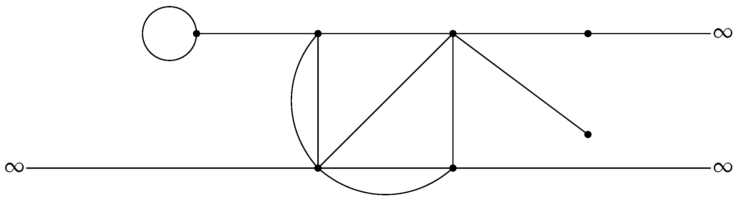
To fix the ideas we start by selecting a collection of points, the vertices of the graph, and a connection rule among them. The bonds joining the vertices are associated to oriented segments and are the finite-length edges of the graph. Other edges can be of infinite length, and these edges are connected only to one vertex and are associated to half-lines. In this way we obtained a metric graph, see, e.g., Figure 1.

Figure 1. A metric graph with seven vertices (marked by dots) and 14 edges (three of which are half-lines).

Given a metric graph $\mathcal{G}$ we denote by $\mathcal{E}$ the set of its edges and by $\mathcal{V}$ the set of its vertices. We shall also use the notation $|\mathcal{E}|$ and $|\mathcal{V}|$ to denote the cardinality of $\mathcal{E}$ and $\mathcal{V}$ respectively. We shall always assume that both $|\mathcal{E}|$ and $|\mathcal{V}|$ are finite.

For any $e\in \mathcal{E}$, we identify the corresponding edge with the segment $[0,{\ell }_e]$ if e has finite length ${\ell }_e>0$, or with $[0,+\infty )$ if e has infinite length.

Given a function $\psi :\mathcal{G}\to \mathbb{C}$, for $e\in \mathcal{E}$, ${\psi }_e$ denotes its restriction to the edge e. With this notation in mind one can define the Hilbert space

$$\mathcal{H}:=\underset{e\in \mathcal{E}}{⨁}{L}^2(e),$$

with scalar product and norm given by

$${(\varphi ,\psi )}_{\mathcal{H}}:=\sum _{e\in \mathcal{E}}{({\varphi }_e,{\psi }_e)}_{L^2(e)}\mathrm{and}{\parallel \psi \parallel }_{\mathcal{H}}:={\left(\psi ,\psi \right)}_{\mathcal{H}}^{1/2}.$$

In a similar way one can define the Sobolev space ${\mathcal{H}}_2:={⨁}_{e\in \mathcal{E}}{H}^2(e)$, equipped with the norm

$${\parallel \psi \parallel }_{{\mathcal{H}}_2}:={\left(\sum _{e\in \mathcal{E}}{\parallel {\psi }_e\parallel }_{H^2(e)}^2\right)}^{1/2}.$$

Note that functions in ${\mathcal{H}}_2$ are continuous in the edges of the graph but do not need to be continuous in the vertices.

For any vertex $v\in \mathcal{V}$ we denote by $d(v)$ the degree of the vertex, this is the number of edges having one endpoint identified by v, counting twice the edges that have both endpoints coinciding with v (loops). Let ${\mathcal{E}}_v\subseteq \mathcal{E}$ be the set of edges which are incident to the vertex v. For any vertex v we order the edges in ${\mathcal{E}}_v$ in an arbitrary way, counting twice the loops. In this way, for an arbitrary function $\psi \in {\mathcal{H}}_2$, one can define the vector $\Psi (v)\in {\mathbb{C}}^{d(v)}$ associated to the evaluation of $\psi$ in v, i.e., the components of $\Psi (v)$ are given by ${\psi }_e(0)$ or ${\psi }_e({\ell }_e)$, $e\in {\mathcal{E}}_v$, depending whether v is the initial or terminal vertex of the edge e, or by both values if e is a loop.

In a similar way one can define the vector ${\Psi }^{\prime }(v)\in {\mathbb{C}}^{d(v)}$ with components ${\psi }_e^{\prime }(0)$ and $-{\psi }_e^{\prime }({\ell }_e)$, $e\in {\mathcal{E}}_v$. Note that in the definition of ${\Psi }^{\prime }(v)$, ${\psi }_e^{\prime }$ denotes the derivative of ${\psi }_e(x)$ with respect to x, and the derivative in v is always taken in the outgoing direction with respect to the vertex.

We are interested in defining self-adjoint operators in $\mathcal{H}$ which coincide with the Laplacian, possibly plus a potential term.

We denote by B the potential term in the operator, so that $B:\mathcal{G}\to \mathbb{R}$ is a real-valued function on the graph; and denote by $B_e$ its restriction to the edge e. Additionally we assume that B is bounded and compactly supported on $\mathcal{G}$.

For every vertex $v\in \mathcal{V}$ we define a projection $P_v:{\mathbb{C}}^{d(v)}\to {\mathbb{C}}^{d(v)}$ and a self-adjoint operator ${\Theta }_v$ in $Ran{P}_v$, both $P_v$ and ${\Theta }_v$ can be identified with Hermitian $d(v)\times d(v)$ matrices.

It is well known, see, e.g., [3] and ([22], Example 5.2) that the operator $H_{P,\Theta }$ defined by:

$$D(H_{P,\Theta }):=\left\{\psi \in {\mathcal{H}}_2|P_v^{\perp }\Psi (v)=0;P_v{\Psi }^{\prime }(v)-{\Theta }_v{P}_v\Psi (v)=0\forall v\in \mathcal{V}\right\}$$

(1)

$${(H_{P,\Theta }\psi )}_e:=-{\psi }_e^{″}+B_e{\psi }_e\forall e\in \mathcal{E}$$

(2)

is self-adjoint. Instead of Equation (2), we shall write

$$H_{P,\Theta }\psi :=-{\psi }^{″}+B\psi ,$$

(3)

to be understood componentwise.

We remark that for every $P_v$ and ${\Theta }_v$ as above, $H_{P,\Theta }$ is a self-adjoint extension of the symmetric operator $H_{min}$

$$D(H_{min}):=\left\{\psi \in {\mathcal{H}}_2|\Psi (v)=0;{\Psi }^{\prime }(v)=0\forall v\in \mathcal{V}\right\}{H}_{min}\psi :=-{\psi }^{″}+B\psi .$$

2.2. Graphs with a Small Compact Core

We consider a graph ${\mathcal{G}}^{\epsilon }$ obtained by attaching several edges to a small compact core (a compact metric graph of size $\epsilon$).

We denote the compact core of the graph by ${\mathcal{G}}^{in,\epsilon }$. The graph ${\mathcal{G}}^{in,\epsilon }$ is obtained by shrinking a compact graph ${\mathcal{G}}^{in}$ by means of a parameter $0<\epsilon <1$, more precisely, we set

$${\mathcal{G}}^{in,\epsilon }=\epsilon {\mathcal{G}}^{in}.$$

(4)

We denote by ${\mathcal{E}}^{in}$ the set of edges of the graph ${\mathcal{G}}^{in}$ and by ${\mathcal{E}}^{in,\epsilon }$ the set of edges of the graph ${\mathcal{G}}^{in,\epsilon }$.

In the graph ${\mathcal{G}}^{in}$ (or, equivalently, in ${\mathcal{G}}^{in,\epsilon }$) we select N distinct vertices that we label with $v_1,\dots ,v_N$, and refer to them as connecting vertices. We shall denote by $\mathcal{C}$ the set of connecting vertices. We denote by ${\mathcal{V}}^{in}$ the set of all the remaining vertices, and call the elements of ${\mathcal{V}}^{in}$inner vertices (note that the set ${\mathcal{V}}^{in}$ may be empty).

To construct the graph ${\mathcal{G}}^{\epsilon }$, we attach to each connecting vertex one additional edge which can be an half-line or an edge of finite length (not dependent on $\epsilon$). We shall call these additional edges outer edges and denote by ${\mathcal{E}}^{out}$ the corresponding set of edges; obviously $|{\mathcal{E}}^{out}|=N$. When needed, we shall denote these edges by $e_1,\dots ,e_N$, so that the edge $e_j$ is connected to the vertex $v_j$, $j=1,\dots ,N$. Moreover we shall use the notation

$${\psi }_{e_j}\equiv {\psi }_j{e}_j\in {\mathcal{E}}^{out},j=1,\dots ,N.$$

Note that if $e\in {\mathcal{E}}^{out}$ is of finite length the endpoint which does not coincide with the connecting vertex is of degree one (all the finite length outer edges are pendants).

We shall always assume, without loss of generality, that for each edge in ${\mathcal{E}}^{out}$ the connecting vertex is identified by $x=0$.

We denote by ${\mathcal{E}}^{\epsilon }$ and $\mathcal{V}$ the sets of edges and vertices of the graph ${\mathcal{G}}^{\epsilon }$. We note that ${\mathcal{E}}^{\epsilon }={\mathcal{E}}^{out}\cup {\mathcal{E}}^{in,\epsilon }$ and $\mathcal{V}={\mathcal{V}}^{out}\cup \mathcal{C}\cup {\mathcal{V}}^{in}$, where ${\mathcal{V}}^{out}$ is the set of vertices in ${\mathcal{G}}^{\epsilon }$ which are neither connecting nor inner vertices.

Remark 1.

For any$v\in \mathcal{C}$we denote by$d^{in}(v)$its degree as a vertex of the graph${\mathcal{G}}^{in,\epsilon }$, so that its degree as a vertex of the graph ${\mathcal{G}}^{\epsilon }$ is $d(v)=d^{in}(v)+1$.

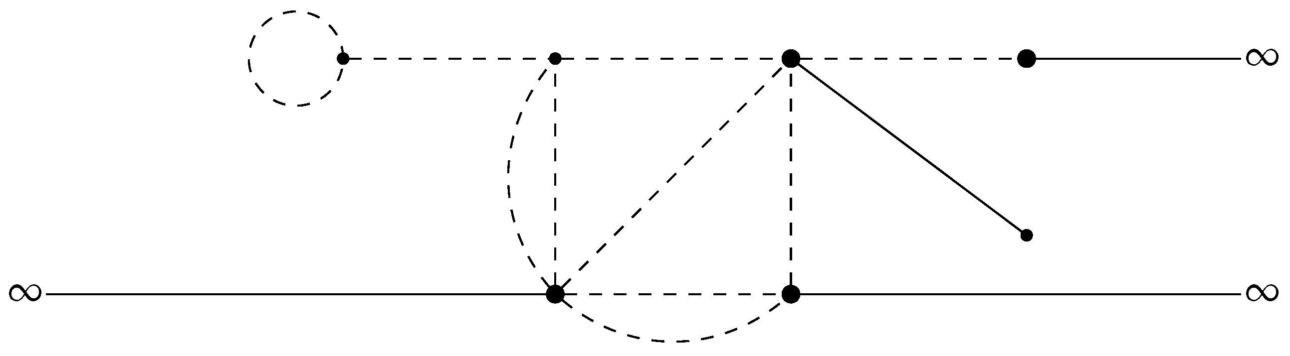
As $\epsilon \to 0$, the inner graph shrinks to one point, in the limit all the connecting vertices merge in one vertex which we identify with the point $x_j=0$, $x_j$ being the coordinate along the edge $e_j\in {\mathcal{E}}^{out}$, $j=1,\dots ,N$. In the limit the graph ${\mathcal{G}}^{\epsilon }$ looks like a star-graph with N edges connected in the origin, see Figure 2; we denote the star-graph by ${\mathcal{G}}^{out}$.

Figure 2. The dashed lines represent the edges of ${\mathcal{G}}^{in,\epsilon }$, the large dots the connecting vertices. The graph ${\mathcal{G}}^{out}$ is obtained by merging the connecting vertices. In the example in the picture, ${\mathcal{G}}^{out}$ has three infinite edges and one edge of finite length.

We define the Hilbert spaces:

$${\mathcal{H}}^{\epsilon }:=\underset{e\in {\mathcal{E}}^{\epsilon }}{⨁}{L}^2(e),{\mathcal{H}}^{out}:=\underset{e\in {\mathcal{E}}^{out}}{⨁}{L}^2(e),{\mathcal{H}}^{in,\epsilon }:=\underset{e\in {\mathcal{E}}^{in,\epsilon }}{⨁}{L}^2(e).$$

We remark that one can always think of ${\mathcal{H}}^{\epsilon }$ as the direct sum

$${\mathcal{H}}^{\epsilon }={\mathcal{H}}^{out}\oplus {\mathcal{H}}^{in,\epsilon },$$

(5)

and decompose each function $\psi \in {\mathcal{H}}^{\epsilon }$ as $\psi =({\psi }^{out},{\psi }^{in})$ with ${\psi }^{out}\in {\mathcal{H}}^{out}$ and ${\psi }^{in}\in {\mathcal{H}}^{in,\epsilon }$. When no misunderstanding is possible, we omit the dependence on $\epsilon$, moreover we simply write $\psi$, instead of ${\psi }^{out}$ or ${\psi }^{in}$.

In a similar way we introduce the Sobolev spaces

$${\mathcal{H}}_2^{\epsilon }:=\underset{e\in {\mathcal{E}}^{\epsilon }}{⨁}{H}^2(e),{\mathcal{H}}_2^{out}:=\underset{e\in {\mathcal{E}}^{out}}{⨁}{H}^2(e),{\mathcal{H}}_2^{in,\epsilon }:=\underset{e\in {\mathcal{E}}^{in,\epsilon }}{⨁}{H}^2(e).$$

2.3. Full Hamiltonian

Next we define an Hamiltonian $H^{\epsilon }$ in ${\mathcal{H}}^{\epsilon }$ (of the form given in Equations (1)–(3)); this is the object of our investigation.

• Recall that if $v\in {\mathcal{V}}^{out}$, then $d(v)=1$. For any $v\in {\mathcal{V}}^{out}$ we fix an orthogonal projection $P_v^{out}:\mathbb{C}\to \mathbb{C}$, and a self-adjoint operator ${\Theta }_v^{out}$ in $Ran(P_v^{out})$. Since vertices in ${\mathcal{V}}^{out}$ have degree one, $P_v^{out}$ is either 1 or 0; whenever $P_v^{out}=1$ it makes sense to define ${\Theta }_v^{out}$ which turns out to be the operator acting as the multiplication by a real constant. In other words, the boundary conditions in $v\in {\mathcal{V}}^{out}$ (of the form given in the definition of $D(H_{P,\Theta })$) can be of Dirichlet type, ${\psi }_e(v)=0$; of Neumann type ${\psi }_e^{\prime }(v)=0$; or of Robin type ${\psi }_e^{\prime }(v)=\alpha {\psi }_e(v)$ with $\alpha \in \mathbb{R}$.
  It would be possible to consider a more general setting in which the outer graph has a non trivial topology, in same spirit of the work [4], but we will not pursue this goal.
• For any $v\in \mathcal{C}$ we define the orthogonal projection (see Remark 1 for the definition of $d(v)$):

  $$K_v:{\mathbb{C}}^{d(v)}\to {\mathbb{C}}^{d(v)},K_v:={\mathbf{1}}_{d(v)}{\left({\mathbf{1}}_{d(v)},·\right)}_{{\mathbb{C}}^{d(v)}}\forall v\in \mathcal{C},$$

  where ${\mathbf{1}}_{d(v)}$ denotes the vector (of unit norm) in ${\mathbb{C}}^{d(v)}$ defined by ${\mathbf{1}}_{d(v)}={(d(v))}^{-1/2}(1,\dots ,1)$. In a similar way, we define the orthogonal projection

  $$K_v^{in}:{\mathbb{C}}^{d^{in}(v)}\to {\mathbb{C}}^{d^{in}(v)},K_v^{in}:={\mathbf{1}}_{d^{in}(v)}{\left({\mathbf{1}}_{d^{in}(v)},·\right)}_{{\mathbb{C}}^{d^{in}(v)}}\forall v\in \mathcal{C},$$

  where ${\mathbf{1}}_{d^{in}(v)}\in {\mathbb{C}}^{d^{in}(v)}$ is defined by ${\mathbf{1}}_{d^{in}(v)}={(d^{in}(v))}^{-1/2}(1,\dots ,1)$. Both $K_v$ and $K_v^{in}$ have one-dimensional range given by the span of the vectors ${\mathbf{1}}_{d(v)}$ and ${\mathbf{1}}_{d^{in}(v)}$ respectively.
  A function $\psi$ satisfies Kirchhoff conditions in the vertex v (it is continuous in v and the sum of the outgoing derivatives in v equals zero) if and only if $K_v^{\perp }\Psi (v)=0$ and $K_v{\Psi }^{\prime }(v)=0$.
• For any $v\in {\mathcal{V}}^{in}$ we fix an orthogonal projection $P_v^{in}:{\mathbb{C}}^{d(v)}\to {\mathbb{C}}^{d(v)}$, and a self-adjoint operator ${\Theta }_v^{in,\epsilon }$ in $Ran(P_v^{in})$.
• We fix an $\epsilon$-dependent real-valued function $B^{\epsilon }:{\mathcal{G}}^{\epsilon }\to \mathbb{R}$, such that in the $out/in$ decomposition (5) one has $B^{\epsilon }=(B^{out},B^{in,\epsilon })$. With $B^{out}:{\mathcal{G}}^{out}\to \mathbb{R}$ bounded and compactly supported.
• Scale invariance; recall that ${\mathcal{G}}^{in,\epsilon }=\epsilon {\mathcal{G}}^{in}$, see Equation (4). We assume additionally: that $B^{in,\epsilon }(x)={\epsilon }^{-2}{B}^{in}(x/\epsilon )$, where $B^{in}:{\mathcal{G}}^{in}\to \mathbb{R}$ is bounded; and that ${\Theta }_v^{in,\epsilon }={\epsilon }^{-1}{\Theta }_v^{in}$, for all $v\in {\mathcal{V}}^{in}$. For a discussion on the meaning and the main consequences of these assumptions we refer to Section 4.

Definition 1 (Hamiltonian H^ε).

We denote by$H^{\epsilon }$the self-adjoint operator in${\mathcal{H}}^{\epsilon }$defined by

$$\begin{array}{cc}\hfill D(H^{\epsilon }):=\{\psi \in {\mathcal{H}}_2^{\epsilon }|& {P_v^{in}}^{\perp }\Psi (v)=0,P_v^{in}{\Psi }^{\prime }(v)-{\Theta }_v^{in,\epsilon }{P}_v^{in}\Psi (v)=0\forall v\in {\mathcal{V}}^{in};\hfill \\ & {P_v^{out}}^{\perp }\Psi (v)=0,P_v^{out}{\Psi }^{\prime }(v)-{\Theta }_v^{out}{P}_v^{out}\Psi (v)=0\forall v\in {\mathcal{V}}^{out};\hfill \\ & K_v^{\perp }\Psi (v)=0,K_v{\Psi }^{\prime }(v)=0\forall v\in \mathcal{C}\}\hfill \end{array}$$

$$H^{\epsilon }\psi :=-{\psi }^{″}+B^{\epsilon }\psi \forall \psi \in D(H^{\epsilon }).$$

Remark 2.

In the$out/in$decomposition one has

$${(H^{\epsilon }\psi )}^{out}=-{{\psi }^{out}}^{″}+B^{out}{\psi }^{out}$$

$${(H^{\epsilon }\psi )}^{in}=-{{\psi }^{in}}^{″}+B^{in,\epsilon }{\psi }^{in}.$$

Note that the action of the outer component of$H^{\epsilon }$does not depend on ε.

Remark 3.

By the definition of$K_v$, in each connecting vertex boundary conditions in$D(H^{\epsilon })$are of Kirchhoff-type: the function ψ is continuous in$v\in \mathcal{C}$and

$$\sum _{e\sim v}{\psi }_e^{\prime }(v)=0v\in \mathcal{C},$$

where the sum is taken on all the edges incident on v (counting loops twice) and the derivative is understood in the outgoing direction from the vertex.

2.4. Auxiliary Hamiltonian

We are interested in the limit of the operator $H^{\epsilon }$ as $\epsilon \to 0$. We shall see that the limiting properties of $H^{\epsilon }$ are strongly related to spectral properties of the Hamiltonian ${\mathring{H}}^{in,\epsilon }$:

Definition 2 (Auxiliary Hamiltonian, scaled down version).

$$\begin{array}{cc}\hfill D({\mathring{H}}^{in,\epsilon }):=\{\psi \in {\mathcal{H}}_2^{in,\epsilon }|& {P_v^{in}}^{\perp }\Psi (v)=0,P_v^{in}{\Psi }^{\prime }(v)-{\Theta }_v^{in,\epsilon }{P}_v^{in}\Psi (v)=0\forall v\in {\mathcal{V}}^{in};\hfill \\ & {K_v^{in}}^{\perp }\Psi (v)=0,K_v^{in}{\Psi }^{\prime }(v)=0\forall v\in \mathcal{C}\}\hfill \end{array}$$

(6)

$${\mathring{H}}^{in,\epsilon }\psi :=-{\psi }^{″}+B^{in,\epsilon }\psi \forall \psi \in D({\mathring{H}}^{in,\epsilon }).$$

Let ${\mathcal{H}}^{in}={\mathcal{H}}^{in,\epsilon =1}$, and define the unitary scaling group

$$U^{in,\epsilon }:{\mathcal{H}}^{in}\to {\mathcal{H}}^{in,\epsilon },(U^{in,\epsilon }{\psi }^{in})(x):={\epsilon }^{-1/2}{\psi }^{in}(x/\epsilon );$$

its inverse is

$${U^{in,\epsilon }}^{-1}:{\mathcal{H}}^{in,\epsilon }\to {\mathcal{H}}^{in},({U^{in,\epsilon }}^{-1}{\psi }^{in})(x)={\epsilon }^{1/2}{\psi }^{in}(\epsilon x).$$

By the scaling properties ${\Theta }_v^{in,\epsilon }={\epsilon }^{-1}{\Theta }_v^{in}$ and $B^{in,\epsilon }(x/\epsilon )={\epsilon }^{-2}{B}^{in}(x)$, one infers the unitary relation

$${\mathring{H}}^{in,\epsilon }={\epsilon }^{-2}{U}^{in,\epsilon }{\mathring{H}}^{in}{U^{in,\epsilon }}^{-1}$$

(7)

with ${\mathring{H}}^{in}$ defined on ${\mathcal{H}}^{\epsilon }$ and given by ${\mathring{H}}^{in}={\mathring{H}}^{in,\epsilon =1}$. One consequence of Equation (7) is that the spectrum of ${\mathring{H}}^{in,\epsilon }$ is related to the spectrum of ${\mathring{H}}^{in}$ by the relation $\sigma ({\mathring{H}}^{in,\epsilon })={\epsilon }^{-2}\sigma ({\mathring{H}}^{in})$ (see Section 4 for more comments on the implications of the scale invariance assumption). For this reason, we prefer to formulate the results in terms of the spectral properties of the $\epsilon$-independent Hamiltonian ${\mathring{H}}^{in}$ instead of the spectral properties of ${\mathring{H}}^{in,\epsilon }$.

Definition 3 (Auxiliary Hamiltonian ${\mathring{H}}^{in}$).

We call Auxiliary Hamiltonian the Hamiltonian${\mathring{H}}^{in}={\mathring{H}}^{in,\epsilon =1}$defined on${\mathcal{H}}^{in}$.

Letting${\mathcal{H}}_2^{in}={\mathcal{H}}_2^{in,\epsilon =1}$, the domain and action of${\mathring{H}}^{in}$are given by

$$\begin{array}{cc}\hfill D({\mathring{H}}^{in})=\{\psi \in {\mathcal{H}}_2^{in}|& {P_v^{in}}^{\perp }\Psi (v)=0,P_v^{in}{\Psi }^{\prime }(v)-{\Theta }_v^{in}{P}_v^{in}\Psi (v)=0\forall v\in {\mathcal{V}}^{in};\hfill \\ & {K_v^{in}}^{\perp }\Psi (v)=0,K_v^{in}{\Psi }^{\prime }(v)=0\forall v\in \mathcal{C}\}\hfill \end{array}$$

(8)

$${\mathring{H}}^{in}\psi =-{\psi }^{″}+B^{in}\psi \forall \psi \in D({\mathring{H}}^{in}).$$

The spectrum of ${\mathring{H}}^{in}$ consists of isolated eigenvalues of finite multiplicity, see, e.g., ([3], Theorem 3.1.1). For $n\in \mathbb{N}$, we denote by ${\lambda }_n$ the eigenvalues of ${\mathring{H}}^{in}$ (counting multiplicity) and by ${\left\{{\phi }_n\right\}}_{n\in \mathbb{N}}$ a corresponding set of orthonormal eigenfunctions.

Definition 4 (Generic/non-generic case).

In the analysis of the limit of$H^{\epsilon }$we distinguish two cases:

(1) 

Generic (or non-resonant, or decoupling) case.$\lambda =0$is not an eigenvalue of the operator${\mathring{H}}^{in}$.

(2) 

Non-generic (or resonant) case.$\lambda =0$is an eigenvalue of the operator${\mathring{H}}^{in}$.

In the non-generic case we denote by${\left\{{\widehat{\phi }}_k\right\}}_{k=1,\dots ,m}$a set of (orthonormal) eigenfunctions corresponding to the zero eigenvalue. By Equation (8), functions in$D({\mathring{H}}^{in})$are continuous in the connecting vertices (see also Remark 3). We denote by${\widehat{\phi }}_k(v)$,$v\in \mathcal{C}$, the value of${\widehat{\phi }}_k$in v, and define the vectors

$${\underline{\widehat{c}}}_k:=({\widehat{\phi }}_k(v_1),\dots ,{\widehat{\phi }}_k(v_N))\in {\mathbb{C}}^N,k=1,\dots ,m,v_j\in \mathcal{C},j=1,\dots ,N.$$

(9)

Definition 5 ($\widehat{C}-\widehat{P}$).

In the non-generic case, let$\widehat{C}$be the operator

$$\widehat{C}:=\sum _{k=1}^m{\underline{\widehat{c}}}_k{({\underline{\widehat{c}}}_k,·)}_{{\mathbb{C}}^N}:{\mathbb{C}}^N\to {\mathbb{C}}^N.$$

$\widehat{C}$is a bounded self-adjoint operator (it is an$N\times N$Hermitian matrix). Denote by$Ran\widehat{C}\subseteq {\mathbb{C}}^N$and$Ker\widehat{C}\subseteq {\mathbb{C}}^N$, the range and the kernel of$\widehat{C}$respectively. One has that the subspaces$Ran\widehat{C}$and$Ker\widehat{C}$are$\widehat{C}$-invariant. Moreover,${\mathbb{C}}^N=Ran\widehat{C}\oplus Ker\widehat{C}$. In what follows we denote by$\widehat{P}$the orthogonal projection (Riesz projection, see, e.g., ([23], Section I.2)) on$Ran(\widehat{C})$, and by${\widehat{P}}^{\perp }={\mathbb{I}}_N-\widehat{P}$the orthogonal projection on$Ker(\widehat{C})$.

Remark 4.

We note that$\underline{q}\in Ker\widehat{C}$if and only if${({\underline{\widehat{c}}}_k,\underline{q})}_{{\mathbb{C}}^N}=0$for all$k=1,\dots ,m$. To see that this indeed the case, observe that if$\underline{q}\in Ker\widehat{C}$then it must be${(\underline{q},\widehat{C}\underline{q})}_{{\mathbb{C}}^N}=0$, hence,${\sum }_{k=1}^m{|{({\underline{\widehat{c}}}_k,\underline{q})}_{{\mathbb{C}}^N}|}^2=0$, which in turn implies${({\underline{\widehat{c}}}_k,\underline{q})}_{{\mathbb{C}}^N}=0$for all$k=1,\dots ,m$. The other implication is trivial.

Since${\widehat{P}}^{\perp }{\underline{\widehat{c}}}_k\in Ker\widehat{C}$, we infer$0={({\underline{\widehat{c}}}_k,{\widehat{P}}^{\perp }{\underline{\widehat{c}}}_k)}_{{\mathbb{C}}^N}={({\widehat{P}}^{\perp }{\underline{\widehat{c}}}_k,{\widehat{P}}^{\perp }{\underline{\widehat{c}}}_k)}_{{\mathbb{C}}^N}={\parallel {\widehat{P}}^{\perp }{\underline{\widehat{c}}}_k\parallel }_{{\mathbb{C}}^N}^2$for all$k=1,\dots ,m$; hence,${\widehat{P}}^{\perp }{\underline{\widehat{c}}}_k=0$, or, equivalently,${\underline{\widehat{c}}}_k\in Ran(\widehat{C})$.

2.5. Effective Hamiltonians

We shall see that the definition of the limiting operator (effective Hamiltonian in ${\mathcal{H}}^{out}$) depends on presence of a zero eigenvalue for ${\mathring{H}}^{in}$ (the occurrence of the generic case vs. the non-generic case).

Recall that for $\psi \in {\mathcal{H}}^{out}$, we used ${\psi }_j$ to denote the component of $\psi$ on the edge $e_j$ attached to the connecting vertex $v_j$. Moreover, we assumed that the vertex $v_j$ is identified by $x=0$. With this remark in mind, given a function $\psi \in {\mathcal{H}}_2^{out}$ we define the vectors

$$\Psi (\mathbf{0}):={({\psi }_1(0),\dots ,{\psi }_N(0))}^T\in {\mathbb{C}}^N,{\Psi }^{\prime }(\mathbf{0}):={({\psi }_1^{\prime }(0),\dots ,{\psi }_N^{\prime }(0))}^T\in {\mathbb{C}}^N.$$

These correspond to $\Psi (v_0)$ and ${\Psi }^{\prime }(v_0)$, as defined in Section 2.1, where $v_0$ is the central vertex of the star-graph ${\mathcal{G}}^{out}$.

In the limit $\epsilon \to 0$, the connecting vertices in ${\mathcal{G}}^{in,\epsilon }$ coincide, and can be identified with the vertex $v_0\equiv \mathbf{0}$.

We distinguish two possible effective Hamiltonians in ${\mathcal{H}}^{out}$.

Definition 6 (Effective Hamiltonian, generic case).

We denote by${\mathring{H}}^{out}$the self-adjoint operator in${\mathcal{H}}^{out}$defined by

$$\begin{array}{cc}\hfill D({\mathring{H}}^{out}):=\{\psi \in {\mathcal{H}}_2^{out}|& {P_v^{out}}^{\perp }\Psi (v)=0,P_v^{out}{\Psi }^{\prime }(v)-{\Theta }_v^{out}{P}_v^{out}\Psi (v)=0\forall v\in {\mathcal{V}}^{out};\hfill \\ & \Psi (\mathbf{0})=0\}\hfill \end{array}$$

(10)

$$H^{out}\psi :=-{\psi }^{″}+B^{out}\psi \forall \psi \in D({\mathring{H}}^{out}).$$

Definition 7 (Effective Hamiltonian, non-generic case).

Let$\widehat{P}$be the orthogonal projection given in Definition 5. We denote by${\widehat{H}}^{out}$the self-adjoint operator in${\mathcal{H}}^{out}$defined by

$$\begin{array}{cc}\hfill D({\widehat{H}}^{out}):=\{\psi \in {\mathcal{H}}_2^{out}|& {P_v^{out}}^{\perp }\Psi (v)=0,P_v^{out}{\Psi }^{\prime }(v)-{\Theta }_v^{out}{P}_v^{out}\Psi (v)=0\forall v\in {\mathcal{V}}^{out};\hfill \\ & {\widehat{P}}^{\perp }\Psi (\mathbf{0})=0,\widehat{P}{\Psi }^{\prime }(\mathbf{0})=0\}\hfill \end{array}$$

$${\widehat{H}}^{out}\psi :=-{\psi }^{″}+B^{out}\psi \forall \psi \in D({\widehat{H}}^{out}).$$

The boundary conditions in $\mathbf{0}$ in the definitions of $D({\mathring{H}}^{out})$ and $D({\widehat{H}}^{out})$ are scale invariant (see ([3], Section 1.4.2)).

2.6. Main Results

In what follows C denotes a generic positive constant independent on $\epsilon$. Given two Hilbert spaces X and Y, we denote by $\mathcal{B}(X,Y)$ (or simply by $\mathcal{B}(X)$ if $X=Y$) the space of bounded linear operators from X to Y, and by ${\parallel ·\parallel }_{\mathcal{B}(X,Y)}$ the corresponding norm. For any $a\in \mathbb{R}$, we use the notation ${\mathcal{O}}_{\mathcal{B}(X,Y)}({\epsilon }^a)$ to denote a generic operator from X to Y whose norm is bounded by $C{\epsilon }^a$ for $\epsilon$ small enough.

Given a bounded operator A in ${\mathcal{H}}^{\epsilon }$ we use the notation

$$A=\left(\begin{array}{cc}{A}^{out,out}& A^{out,in}\\ A^{in,out}& A^{in,in}\end{array}\right)$$

(11)

to describe its action in the $out/in$ decomposition (5): here $A^{u,v}:{\mathcal{H}}^v\to {\mathcal{H}}^u$, $u,v=out,in$, are operators defined according to

$$\begin{array}{cc}\hfill {(A\psi )}^{out}=& A^{out,out}{\psi }^{out}+A^{out,in}{\psi }^{in}\hfill \\ \hfill {(A\psi )}^{in}=& A^{in,out}{\psi }^{out}+A^{in,in}{\psi }^{in}.\hfill \end{array}$$

(12)

Theorem 1.

Let$z\in \mathbb{C}\setminus \mathbb{R}$. In the generic case (see Definition 4)

$${(H^{\epsilon }-z)}^{-1}=\left(\begin{array}{cc}{({\mathring{H}}^{out}-z)}^{-1}& \mathbb{O}\\ \mathbb{O}& \mathbb{O}\end{array}\right)+{\mathcal{O}}_{\mathcal{B}({\mathcal{H}}^{\epsilon })}(\epsilon ),$$

(13)

where the expansion has to be understood in the$out/in$decomposition (11).

Theorem 2.

Let$z\in \mathbb{C}\setminus \mathbb{R}$. In the non-generic case (see Definition 4), let${\widehat{C}}_0$be the restriction of$\widehat{C}$to$Ran\widehat{P}$.

(i) 

If$Ker\widehat{C}\subset {\mathbb{C}}^N$,${\widehat{C}}_0$is invertible as an operator in$\widehat{P}{\mathbb{C}}^N$, and

$${(H^{\epsilon }-z)}^{-1}=\left(\begin{array}{cc}{({\widehat{H}}^{out}-z)}^{-1}& \mathbb{O}\\ \mathbb{O}& -z^{-1}{\sum }_{k,k^{\prime }=1}^m\left({\delta }_{k,k^{\prime }}-{({\underline{\widehat{c}}}_k,{\widehat{C}}_0^{-1}{\underline{\widehat{c}}}_{k^{\prime }})}_{{\mathbb{C}}^N}\right){\widehat{\phi }}_k^{\epsilon }{({\widehat{\phi }}_{k^{\prime }}^{\epsilon },·)}_{{\mathcal{H}}^{in,\epsilon }}\end{array}\right)+{\mathcal{O}}_{\mathcal{B}({\mathcal{H}}^{\epsilon })}({\epsilon }^{1/2}),$$

(14)

where the expansion has to be understood in the$out/in$decomposition (11).

(ii) 

If$Ker\widehat{C}={\mathbb{C}}^N$, then$\widehat{P}=0$, and expansion (14) holds true with${\widehat{H}}^{out}={\mathring{H}}^{out}$,${({\underline{\widehat{c}}}_k,{\widehat{C}}_0^{-1}{\underline{\widehat{c}}}_{k^{\prime }})}_{{\mathbb{C}}^N}=0$for all$k,k^{\prime }=1,\dots ,m$, and the error term changed in${\mathcal{O}}_{\mathcal{B}({\mathcal{H}}^{\epsilon })}(\epsilon )$.

(iii) 

If the vectors${\underline{\widehat{c}}}_k$,$k=1,\dots ,m$, are linearly independent, then$\left({\delta }_{k,k^{\prime }}-{({\underline{\widehat{c}}}_k,{\widehat{C}}_0^{-1}{\underline{\widehat{c}}}_{k^{\prime }})}_{{\mathbb{C}}^N}\right)=0$for all$k,k^{\prime }=1,\dots ,m$, and

$${(H^{\epsilon }-z)}^{-1}=\left(\begin{array}{cc}{({\widehat{H}}^{out}-z)}^{-1}& \mathbb{O}\\ \mathbb{O}& \mathbb{O}\end{array}\right)+{\mathcal{O}}_{\mathcal{B}({\mathcal{H}}^{\epsilon })}({\epsilon }^{1/2}).$$

(15)

Remark 5.

Finer estimates on the remainders in Equations (13) and (14) are given in Theorems 3 and 4 below.

Remark 6.

We recall and adapt to our setting the notion of${\delta }^{\epsilon }$-quasi unitary equivalence of operators acting on different Hilbert spaces introduced by P. Exner and O. Post, see in particular ([7], Section 3.2) and ([9], Chapter 4). See also ([4], Section 5) for a discussion on the application of this approach to the analysis of operators on graphs with shrinking edges.

Let J be the operator

$$J:{\mathcal{H}}^{out}\to {\mathcal{H}}^{\epsilon },J{\psi }^{out}=({\psi }^{out},0)\mathit{for}\mathit{all}{\psi }^{out}\in {\mathcal{H}}^{out},$$

where$({\psi }^{out},0)$is understood in the decomposition (5). Its adjoint$J^{\ast }$maps${\mathcal{H}}^{\epsilon }$in${\mathcal{H}}^{out}$, and is given by:

$$J^{\ast }:{\mathcal{H}}^{\epsilon }\to {\mathcal{H}}^{out},J^{\ast }\psi ={\psi }^{out}\mathit{for}\mathit{all}\psi =({\psi }^{out},{\psi }^{in})\in {\mathcal{H}}^{\epsilon }.$$

Note that$J^{\ast }J={\mathbb{I}}^{out}$, where${\mathbb{I}}^{out}$is the identity in${\mathcal{H}}^{out}$.

The operator$H^{\epsilon }$is${\delta }^{\epsilon }$-quasi unitarily equivalent to a self-adjoint operator$H^{out}$in${\mathcal{H}}^{out}$if

$$\parallel (\mathbb{I}-J{J}^{\ast }){(H^{\epsilon }-z)}^{-1}{\parallel }_{\mathcal{B}({\mathcal{H}}^{\epsilon })}\le C{\delta }^{\epsilon }\mathit{and}\parallel J{(H^{out}-z)}^{-1}-{(H^{\epsilon }-z)}^{-1}J{\parallel }_{\mathcal{B}({\mathcal{H}}^{out},{\mathcal{H}}^{\epsilon })}\le C{\delta }^{\epsilon },$$

(16)

for some$z\in \mathbb{C}\setminus \mathbb{R}$.

Note that in the decomposition (12), one has

$$(\mathbb{I}-J{J}^{\ast }){(H^{\epsilon }-z)}^{-1}\psi ={\left({(H^{\epsilon }-z)}^{-1}\right)}^{in,out}{\psi }^{out}+{\left({(H^{\epsilon }-z)}^{-1}\right)}^{in,in}{\psi }^{in}$$

and

$$(J{(H^{out}-z)}^{-1}-{(H^{\epsilon }-z)}^{-1}J){\psi }^{out}=\left(\left({(H^{out}-z)}^{-1}-{\left({(H^{\epsilon }-z)}^{-1}\right)}^{out,out}\right){\psi }^{out},-{\left({(H^{\epsilon }-z)}^{-1}\right)}^{in,out}{\psi }^{out}\right),$$

hence:

By Theorem 1, in the generic case the operator$H^{\epsilon }$is ε-quasi unitarily equivalent to the operator${\mathring{H}}^{out}$.

By Theorem 2–(iii), in the non-generic case, if the vectors${\underline{\widehat{c}}}_k$,$k=1,\dots ,m$, are linearly independent, the operator$H^{\epsilon }$is${\epsilon }^{1/2}$-quasi unitarily equivalent to the operator${\widehat{H}}^{out}$. More precisely, the second condition in Equation (16) always holds true, while the first one holds true only under the additional assumption that the vectors${\underline{\widehat{c}}}_k$are linearly independent.

We refer to [9] for a comprehensive discussion on the comparison between operators acting on different spaces.

3. Kreĭn Resolvent Formulae

In this section we introduce the main tools in our analysis: the Kreĭn-type resolvent formulae for the resolvents of $H^{\epsilon }$ and ${\widehat{H}}^{out}$. The proofs are postponed to Appendix A.

Given the Hilbert spaces $X^{out}$, $Y^{out}$, $X^{in}$, and $Y^{in}$, and a couple of operators $A^{out}:X^{out}\to Y^{out}$ and $A^{in}:X^{in}\to Y^{in}$, we denote by $A:=diag(A^{out},A^{in})$, the operator $A:X\to Y$, with $X:=X^{out}\oplus X^{in}$ and $Y:=Y^{out}\oplus Y^{in}$, acting as $Af:=(A^{out}{f}^{out},A^{in}{f}^{in})$, for all $f=(f^{out},f^{in})\in X$, $f^{out}\in X^{out}$ and $f^{in}\in X^{in}$.

We set

$$D({\mathring{H}}^{\epsilon }):=D({\mathring{H}}^{out})\oplus D({\mathring{H}}^{in,\epsilon })\mathrm{and}{\mathring{H}}^{\epsilon }:=diag({\mathring{H}}^{out},{\mathring{H}}^{in,\epsilon }),$$

(17)

with ${\mathring{H}}^{out}$ and ${\mathring{H}}^{in,\epsilon }$ given as in Definitions 6 and 2.

Given an operator A, we denote by $\rho (A)$ its resolvent set; the resolvent of A is defined as ${(A-z)}^{-1}$ for all $z\in \rho (A)$.

For the resolvents of the relevant operators we introduce the shorthand notation

$$R_z^{\epsilon }:={(H^{\epsilon }-z)}^{-1}z\in \rho (H^{\epsilon });$$

(18)

$${\mathring{R}}_z^{\epsilon }:={({\mathring{H}}^{\epsilon }-z)}^{-1}z\in \rho ({\mathring{H}}^{\epsilon })=\rho ({\mathring{H}}^{out})\cap \rho ({\mathring{H}}^{in,\epsilon });$$

(19)

$${\mathring{R}}_z^{out}:={({\mathring{H}}^{out}-z)}^{-1}z\in \rho ({\mathring{H}}^{out});{\widehat{R}}_z^{out}:={({\widehat{H}}^{out}-z)}^{-1}z\in \rho ({\widehat{H}}^{out});$$

(20)

$${\mathring{R}}_z^{in,\epsilon }:={({\mathring{H}}^{in,\epsilon }-z)}^{-1}z\in \rho ({\mathring{H}}^{in,\epsilon }).$$

(21)

Obviously, all the operators in Equations (18)–(21) are well-defined and bounded for $z\in \mathbb{C}\setminus \mathbb{R}$, moreover ${\mathring{R}}_z^{\epsilon }=diag({\mathring{R}}_z^{out},{\mathring{R}}_z^{in,\epsilon })$.

Our aim is to write the resolvent difference $R_z^{\epsilon }-{\mathring{R}}_z^{\epsilon }$ in a suitable block matrix form, associated to the off-diagonal matrix $\Theta$ in Equation (29). To do so we follow the approach of Posilicano [22,24]. All the self-adjoint extensions of the symmetric operator obtained by restricting a given self-adjoint operator to the kernel of a given map $\tau$ are parametrized by a projection $\mathbf{P}$ and a self-adjoint operator $\Theta$ in $Ran\mathbf{P}$. We choose the reference operator ${\mathring{H}}^{\epsilon }$ and the map $\tau$ so that the Hamiltonian of interest $H^{\epsilon }$ is the self-adjoint extension parametrized by the identity and the self-adjoint operator given by the off-diagonal matrix $\Theta$. The Kreĭn formula for the resolvent difference $R_z^{\epsilon }-{\mathring{R}}_z^{\epsilon }$, see Lemma 2, is obtained within the approach from [22,24].

We define the maps:

$${\tau }^{out}:{\mathcal{H}}_2^{out}\to {\mathbb{C}}^N{\tau }^{out}\psi :={\Psi }^{\prime }(\mathbf{0});$$

(22)

$$\begin{array}{c}{\tau }^{in}:{\mathcal{H}}_2^{in,\epsilon }\to {\mathbb{C}}^N\hfill \\ {\tau }^{in}\psi :={\left(\frac{1}{\sqrt{d^{in}(v_1)}}{({\mathbf{1}}_{d^{in}(v_1)},\Psi (v_1))}_{{\mathbb{C}}^{d^{in}(v_1)}},\dots ,\frac{1}{\sqrt{d^{in}(v_N)}}{({\mathbf{1}}_{d^{in}(v_N)},\Psi (v_N))}_{{\mathbb{C}}^{d^{in}(v_N)}}\right)}^T.\hfill \end{array}$$

(23)

Moreover we set,

$$\tau :{\mathcal{H}}_2^{\epsilon }={\mathcal{H}}_2^{out}\oplus {\mathcal{H}}_2^{in,\epsilon }\to {\mathbb{C}}^{2N}\tau :=diag({\tau }^{out},{\tau }^{in}).$$

Note that we are using the identification ${\mathbb{C}}^{2N}={\mathbb{C}}^N\oplus {\mathbb{C}}^N$.

The following maps are well-defined and bounded

$${\breve{G}}_z^{out}:{\mathcal{H}}^{out}\to {\mathbb{C}}^N{\breve{G}}_z^{out}:={\tau }^{out}{\mathring{R}}_z^{out}z\in \rho ({\mathring{H}}^{out})$$

and

$${\breve{G}}_z^{in,\epsilon }:{\mathcal{H}}^{in,\epsilon }\to {\mathbb{C}}^N{\breve{G}}_z^{in,\epsilon }:={\tau }^{in}{\mathring{R}}_z^{in,\epsilon }z\in \rho ({\mathring{H}}^{in,\epsilon }).$$

(24)

Moreover we set

$${\breve{G}}_z^{\epsilon }:{\mathcal{H}}^{\epsilon }={\mathcal{H}}^{out}\oplus {\mathcal{H}}^{in,\epsilon }\to {\mathbb{C}}^{2N}{\breve{G}}_z^{\epsilon }:=diag({\breve{G}}_z^{out},{\breve{G}}_z^{in,\epsilon }),$$

for $z\in \rho ({\mathring{H}}^{out})\cap \rho ({\mathring{H}}^{in,\epsilon })$. Note that ${\breve{G}}_z^{\epsilon }=\tau {\mathring{R}}_z^{\epsilon }$ and that all the maps above are well-defined bounded operators for $z\in \mathbb{C}\setminus \mathbb{R}$.

The adjoint maps (in $\overline{z}$) are denoted by

$$G_z^{out}:{\mathbb{C}}^N\to {\mathcal{H}}^{out}{G}_z^{out}:={\breve{G}}_{\overline{z}}^{out\ast },$$

$$G_z^{in,\epsilon }:{\mathbb{C}}^N\to {\mathcal{H}}^{in,\epsilon }{G}_z^{in,\epsilon }:={\breve{G}}_{\overline{z}}^{in,\epsilon \ast },$$

(25)

(${}^{\ast }$ denoting the adjoint) and

$$G_z^{\epsilon }:{\mathbb{C}}^{2N}\to {\mathcal{H}}^{\epsilon }{G}_z^{\epsilon }:={\breve{G}}_{\overline{z}}^{\epsilon \ast }.$$

Obviously $G_z^{\epsilon }=diag(G_z^{out},G_z^{in,\epsilon })$ to be understood as an operator from ${\mathbb{C}}^{2N}={\mathbb{C}}^N\oplus {\mathbb{C}}^N$ to ${\mathcal{H}}^{\epsilon }={\mathcal{H}}^{out}\oplus {\mathcal{H}}^{in,\epsilon }$.

We note that, see Remark A2, $G_z^{out}:{\mathbb{C}}^N\to {\mathcal{H}}_2^{out}$ and $G_z^{in,\epsilon }:{\mathbb{C}}^N\to {\mathcal{H}}_2^{in,\epsilon }$, for all $z\in \rho ({\mathring{H}}^{out})$ and $z\in \rho ({\mathring{H}}^{in,\epsilon })$ respectively, so that the maps ($N\times N$, z-dependent matrices)

$$M_z^{out}:{\mathbb{C}}^N\to {\mathbb{C}}^N,M_z^{out}:={\tau }^{out}{G}_z^{out}z\in \rho ({\mathring{H}}^{out})$$

(26)

$$M_z^{in,\epsilon }:{\mathbb{C}}^N\to {\mathbb{C}}^N,M_z^{in,\epsilon }:={\tau }^{in}{G}_z^{in,\epsilon }z\in \rho ({\mathring{H}}^{in,\epsilon }),$$

(27)

are well defined. Moreover, we set

$$M_z^{\epsilon }:{\mathbb{C}}^{2N}\to {\mathbb{C}}^{2N},M_z^{\epsilon }:=diag(M_z^{out},M_z^{in,\epsilon })z\in \rho ({\mathring{H}}^{out})\cap \rho ({\mathring{H}}^{in,\epsilon })=\rho ({\mathring{H}}^{\epsilon });$$

(28)

obviously $M_z^{\epsilon }=\tau G^{\epsilon }(z)$.

In the following Lemmata we give two Kreĭn-type resolvent formulae: one allows to express the resolvent of ${\widehat{H}}^{out}$ in terms of the resolvent of ${\mathring{H}}^{out}$; the other gives the resolvent of $H^{\epsilon }$ in terms of the resolvent of ${\mathring{H}}^{\epsilon }$. For the proofs we refer to Appendix A, Appendix A.1.

Lemma 1.

Let$\widehat{P}$be an orthogonal projection in${\mathbb{C}}^N$, and${\widehat{H}}^{out}$and${\mathring{H}}^{out}$be the Hamiltonians defined according to Definitions 7 and 6. Then, for any$z\in \rho ({\widehat{H}}^{out})\cap \rho ({\mathring{H}}^{out})$, the map$\widehat{P}{M}_z^{out}\widehat{P}:\widehat{P}{\mathbb{C}}^N\to \widehat{P}{\mathbb{C}}^N$is invertible and

$${\widehat{R}}_z^{out}={\mathring{R}}_z^{out}-G_z^{out}\widehat{P}{\left(\widehat{P}{M}_z^{out}\widehat{P}\right)}^{-1}\widehat{P}{\breve{G}}_z^{out}.$$

Lemma 2.

Let Θ be the $2N\times 2N$ block matrix

$$\Theta =\left(\begin{array}{cc}{\mathbb{O}}_N& {\mathbb{I}}_N\\ {\mathbb{I}}_N& {\mathbb{O}}_N\end{array}\right).$$

(29)

Then, for any$z\in \rho (H^{\epsilon })\cap \rho ({\mathring{H}}^{\epsilon })$, the map$(M_z^{\epsilon }-\Theta ):{\mathbb{C}}^{2N}\to {\mathbb{C}}^{2N}$is invertible and

$$R_z^{\epsilon }={\mathring{R}}_z^{\epsilon }-G_z^{\epsilon }{\left(M_z^{\epsilon }-\Theta \right)}^{-1}{\breve{G}}_z^{\epsilon }.$$

We conclude this section with an alternative formula for the resolvent $R_z^{\epsilon }$. We refer to Appendix A, Appendix A.2, for the proof.

Lemma 3.

Let$z\in \mathbb{C}\setminus \mathbb{R}$, then the maps ($N\times N$, z-dependent matrices)

$$M_z^{in,\epsilon }{M}_z^{out}-{\mathbb{I}}_N:{\mathbb{C}}^N\to {\mathbb{C}}^N\mathit{and}{M}_z^{out}{M}_z^{in,\epsilon }-{\mathbb{I}}_N:{\mathbb{C}}^N\to {\mathbb{C}}^N$$

(30)

are invertible. Moreover,

$$R_z^{\epsilon }={\mathring{R}}_z^{\epsilon }-G_z^{\epsilon }\left(\begin{array}{cc}{\left(M_z^{in,\epsilon }{M}_z^{out}-{\mathbb{I}}_N\right)}^{-1}{M}_z^{in,\epsilon }& {\left(M_z^{in,\epsilon }{M}_z^{out}-{\mathbb{I}}_N\right)}^{-1}\\ {\left(M_z^{out}{M}_z^{in,\epsilon }-{\mathbb{I}}_N\right)}^{-1}& M_z^{out}{\left(M_z^{in,\epsilon }{M}_z^{out}-{\mathbb{I}}_N\right)}^{-1}\end{array}\right){\breve{G}}_z^{\epsilon }.$$

(31)

4. Scale Invariance

In this section we discuss the scale invariance properties of ${\mathring{H}}^{in,\epsilon }$ and collect several formulae concerning the operators ${\mathring{R}}_z^{in,\epsilon }$, ${\breve{G}}_z^{in,\epsilon }$, $G_z^{in,\epsilon }$, and $M_z^{in,\epsilon }$.

Recall that we have denoted by ${\lambda }_n$ and ${\left\{{\phi }_n\right\}}_{n\in \mathbb{N}}$ the eigenvalues and a corresponding set of orthonormal eigenfunctions of ${\mathring{H}}^{in}$.

The eigenvalues of ${\mathring{H}}^{in,\epsilon }$ (counting multiplicity) and a corresponding set of orthonormal eigenfunctions are given by

$${\lambda }_n^{\epsilon }={\epsilon }^{-2}{\lambda }_n;{\phi }_n^{\epsilon }(x)={\epsilon }^{-1/2}{\phi }_n(x/\epsilon ),$$

(32)

where ${\lambda }_n$ are the eigenvalues of ${\mathring{H}}^{in}$, and ${\phi }_n$ the corresponding (orthonormal) eigenfunctions.

By the spectral theorem and by the scaling properties (32), ${\mathring{R}}_z^{in,\epsilon }$ is given by

$${\mathring{R}}_z^{in,\epsilon }=\sum _{n\in \mathbb{N}}\frac{{\phi }_n^{\epsilon }{({\phi }_n^{\epsilon },·)}_{{\mathcal{H}}^{in,\epsilon }}}{{\lambda }_n^{\epsilon }-z}={\epsilon }^2\sum _{n\in \mathbb{N}}\frac{{\phi }_n^{\epsilon }{({\phi }_n^{\epsilon },·)}_{{\mathcal{H}}^{in,\epsilon }}}{{\lambda }_n-{\epsilon }^{2}z}.$$

(33)

Hence, its integral kernel can be written as

$${\mathring{R}}_z^{in,\epsilon }(x,y)=\epsilon \sum _{n\in \mathbb{N}}\frac{{\phi }_n(x/\epsilon ){\phi }_n(y/\epsilon )}{{\lambda }_n-{\epsilon }^{2}z}x,y\in {\mathcal{G}}^{in,\epsilon }.$$

(34)

Since there exists a positive constant C such that ${sup}_{x\in {\mathcal{G}}^{in}}|{\phi }_n(x)|\le C$ and ${\lambda }_n\ge C{n}^2$ for n large enough (see Appendix B), the series in Equation (34) is uniformly convergent for $x,y\in {\mathcal{G}}^{in,\epsilon }$. Hence, we can write the operators ${\breve{G}}_z^{in,\epsilon }$ and $G_z^{in,\epsilon }$, and the matrix $M_z^{in,\epsilon }$ in a similar way, see Equations (35) and (36) below.

Note that, since functions in $D({\mathring{H}}^{in,\epsilon })$ are continuous in the connecting vertices, the eigenfunctions ${\phi }_n^{\epsilon }$ can be evaluated in the connecting vertices, and, by the definition of ${\tau }^{in}$ (see Equation (23)), one has

$${\tau }^{in}{\phi }_n^{\epsilon }={({\phi }_n^{\epsilon }(v_1),\dots ,{\phi }_n^{\epsilon }(v_N))}^T.$$

So that, for any eigenfunction ${\phi }_n^{\epsilon }$ we can define the vector ${\underline{c}}_n^{\epsilon }$ as

$${\underline{c}}_n^{\epsilon }:={\tau }^{in}{\phi }_n^{\epsilon }.$$

We note that ${\underline{c}}_n^{\epsilon }={\epsilon }^{-1/2}{\underline{c}}_n$, with

$${\underline{c}}_n={\left({\phi }_n(v_1),\dots ,{\phi }_n(v_N)\right)}^T,$$

and that the vectors ${\underline{c}}_n$ are defined in the same way as the vectors ${\underline{\widehat{c}}}_k$ in Equation (9).

Remark 7.

In the non-generic case, zero is an eigenvalue of${\mathring{H}}^{in,\epsilon }$. We denote by${\left\{{\widehat{\phi }}_k^{\epsilon }\right\}}_{k=1,\dots ,m}$the corresponding set of (orthonormal) eigenfunctions given by${\widehat{\phi }}_k^{\epsilon }(x)={\epsilon }^{-1/2}{\widehat{\phi }}_k(x/\epsilon )$where${\widehat{\phi }}_k$are the eigenfunctions corresponding to the eigenvalue zero of${\mathring{H}}^{in}$. The vectors${\underline{\widehat{c}}}_k^{\epsilon }:={\tau }^{in}{\widehat{\phi }}_k^{\epsilon }$are related to the vectors${\underline{\widehat{c}}}_k$by the identity${\underline{\widehat{c}}}_k^{\epsilon }={\epsilon }^{-1/2}{\underline{\widehat{c}}}_k$.

By the discussion above, and by the definitions (24), (25), and (27), we obtain

$${\breve{G}}_z^{in,\epsilon }={\epsilon }^{3/2}\sum _{n\in \mathbb{N}}\frac{{\underline{c}}_n{({\phi }_n^{\epsilon },·)}_{{\mathcal{H}}^{in,\epsilon }}}{{\lambda }_n-{\epsilon }^{2}z};G_z^{in,\epsilon }={\epsilon }^{3/2}\sum _{n\in \mathbb{N}}\frac{{\phi }_n^{\epsilon }{({\underline{c}}_n,·)}_{{\mathbb{C}}^N}}{{\lambda }_n-{\epsilon }^{2}z},$$

(35)

and

$$M_z^{in,\epsilon }=\epsilon \sum _{n\in \mathbb{N}}\frac{{\underline{c}}_n{({\underline{c}}_n,·)}_{{\mathbb{C}}^N}}{{\lambda }_n-{\epsilon }^{2}z}.$$

(36)

5. Proof of Theorems 1 and 2

This section is devoted to the proofs of Theorems 1 and 2. Actually, we shall prove a finer version of the results with more precise estimates of the remainders, see Theorems 3 and 4 below.

Remark 8.

By Equation (31), it follows that, in the$out/in$decomposition (11), the resolvent$R_z^{\epsilon }$can be written as

$$R_z^{\epsilon }=\left(\begin{array}{cc}{\mathring{R}}_z^{out}& \mathbb{O}\\ \mathbb{O}& {\mathring{R}}_z^{in,\epsilon }\end{array}\right)-\left(\begin{array}{cc}{\mathcal{R}}_z^{out,out,\epsilon }& {\mathcal{R}}_z^{out,in,\epsilon }\\ {\mathcal{R}}_z^{in,out,\epsilon }& {\mathcal{R}}_z^{in,in,\epsilon }\end{array}\right)$$

(37)

with

$$\begin{array}{cc}\hfill {\mathcal{R}}_z^{out,out,\epsilon }& =G_z^{out}{\left(M_z^{in,\epsilon }{M}_z^{out}-{\mathbb{I}}_N\right)}^{-1}{M}_z^{in,\epsilon }{\breve{G}}_z^{out};\hfill \end{array}$$

(38)

$$\begin{array}{cc}\hfill {\mathcal{R}}_z^{in,out,\epsilon }& =G_z^{in,\epsilon }{\left(M_z^{out}{M}_z^{in,\epsilon }-{\mathbb{I}}_N\right)}^{-1}{\breve{G}}_z^{out};\hfill \end{array}$$

(39)

$$\begin{array}{cc}\hfill {\mathcal{R}}_z^{out,in,\epsilon }& =G_z^{out}{\left(M_z^{in,\epsilon }{M}_z^{out}-{\mathbb{I}}_N\right)}^{-1}{\breve{G}}_z^{in,\epsilon };\hfill \end{array}$$

(40)

$$\begin{array}{cc}\hfill {\mathcal{R}}_z^{in,in,\epsilon }& =G_z^{in,\epsilon }{M}_z^{out}{\left(M_z^{in,\epsilon }{M}_z^{out}-{\mathbb{I}}_N\right)}^{-1}{\breve{G}}_z^{in,\epsilon }.\hfill \end{array}$$

(41)

Note that since$M_z=M_{\overline{z}}^{\ast }$holds true both for the “$out$” and “$in$” M-matrices (see Equation (A2)), one infers${\mathcal{R}}_z^{in,out,\epsilon }={\mathcal{R}}_{\overline{z}}^{out,in,\epsilon \ast }$.

5.1. Generic Case. Proof of Theorem 1

In this section we study the limit of the relevant quantities in the generic case and prove Theorem 1.

Proposition 1.

Let$z\in \mathbb{C}\setminus \mathbb{R}$. In the generic case,

$${\mathring{R}}_z^{in,\epsilon }={\mathcal{O}}_{\mathcal{B}({\mathcal{H}}^{in,\epsilon })}({\epsilon }^2);$$

(42)

$${\breve{G}}_z^{in,\epsilon }={\mathcal{O}}_{\mathcal{B}({\mathcal{H}}^{in,\epsilon },{\mathbb{C}}^N)}({\epsilon }^{3/2});G_z^{in,\epsilon }={\mathcal{O}}_{\mathcal{B}({\mathbb{C}}^N,{\mathcal{H}}^{in,\epsilon })}({\epsilon }^{3/2}).$$

(43)

Proof. 

We prove first Claim (42). For any ${\psi }^{in}\in {\mathcal{H}}^{in,\epsilon }$, since ${\left\{{\phi }_n^{\epsilon }\right\}}_{n\in \mathbb{N}}$ is an orthonormal set of eigenfunctions in ${\mathcal{H}}^{in,\epsilon }$, and by Equation (33), we infer

$$\parallel {\mathring{R}}_z^{in,\epsilon }{\psi }^{in}{\parallel }_{{\mathcal{H}}^{in,\epsilon }}={\epsilon }^2{\left(\sum _{n\in \mathbb{N}}\frac{|{({\phi }_n^{\epsilon },{\psi }^{in})}_{{\mathcal{H}}^{in,\epsilon }}{|}^2}{|{\lambda }_n-{\epsilon }^2{z|}^2}\right)}^{1/2}\le C{\epsilon }^2{\parallel {\psi }^{in}\parallel }_{{\mathcal{H}}^{in,\epsilon }},$$

where in the latter inequality we used the bound $|{\lambda }_n-{\epsilon }^2{z|}^{-2}\le 4{|{\lambda }_n|}^{-2}\le C$, which holds true in the generic case because $|{\lambda }_n-{\epsilon }^{2}z|\ge |{\lambda }_n|/2\ge C$ for all $n\in \mathbb{N}$ and $\epsilon$ small enough.

To prove the first claim in Equation (43), let ${\psi }^{in}\in {\mathcal{H}}^{in,\epsilon }$, then

$${\breve{G}}_z^{in,\epsilon }{\psi }^{in}={\epsilon }^{3/2}\sum _{n\in \mathbb{N}}\frac{{\underline{c}}_n{({\phi }_n^{\epsilon },{\psi }^{in})}_{{\mathcal{H}}^{in,\epsilon }}}{{\lambda }_n-{\epsilon }^{2}z}.$$

Hence, from the Cauchy–Schwarz inequality,

$$\begin{array}{cc}\hfill \parallel {\breve{G}}_z^{in,\epsilon }{\psi }^{in}{\parallel }_{{\mathbb{C}}^N}\le & {\epsilon }^{3/2}\sum _{n\in \mathbb{N}}\frac{\parallel {\underline{c}}_n{\parallel }_{{\mathbb{C}}^N}|{({\phi }_n^{\epsilon },{\psi }^{in})}_{{\mathcal{H}}^{in,\epsilon }}|}{|{\lambda }_n-{\epsilon }^{2}z|}\hfill \\ \hfill \le & {\epsilon }^{3/2}\parallel {\psi }^{in}{\parallel }_{{\mathcal{H}}^{in,\epsilon }}{\left(\sum _{n\in \mathbb{N}}\frac{\parallel {\underline{c}}_n{\parallel }_{{\mathbb{C}}^N}^2}{|{\lambda }_n-{\epsilon }^2{z|}^2}\right)}^{1/2}\le C{\epsilon }^{3/2}{\parallel {\psi }^{in}\parallel }_{{\mathcal{H}}^{in,\epsilon }},\hfill \end{array}$$

because $\parallel {\underline{c}}_n{\parallel }_{{\mathbb{C}}^N}^2\le C$ and ${\sum }_{n\in \mathbb{N}}|{\lambda }_n-{\epsilon }^2{z|}^{-2}\le C{\sum }_{n\in \mathbb{N}}{|{\lambda }_n|}^{-2}\le C$. This proves the first Claim in Equation (43); the second one is trivial, being $G_z^{in,\epsilon }$ the adjoint of ${\breve{G}}_{\overline{z}}^{in,\epsilon }$. □

Proposition 2.

Let$z\in \mathbb{C}\setminus \mathbb{R}$. In the generic case,

$$M_z^{in,\epsilon }={\mathcal{O}}_{\mathcal{B}({\mathbb{C}}^N)}(\epsilon ).$$

(44)

Proof. 

Recall Equation (36) and note that for any $\underline{q}\in {\mathbb{C}}^N$,

$$\parallel M_z^{in,\epsilon }\underline{q}{\parallel }_{{\mathbb{C}}^N}\le \epsilon \sum _{n\in \mathbb{N}}\frac{\parallel {\underline{c}}_n{\parallel }_{{\mathbb{C}}^N}|{({\underline{c}}_n,\underline{q})}_{{\mathbb{C}}^N}|}{|{\lambda }_n-{\epsilon }^{2}z|}\le \epsilon \parallel \underline{q}{\parallel }_{{\mathbb{C}}^N}\sum _{n\in \mathbb{N}}\frac{\parallel {\underline{c}}_n{\parallel }_{{\mathbb{C}}^N}^2}{|{\lambda }_n-{\epsilon }^{2}z|}\le C\epsilon {\parallel \underline{q}\parallel }_{{\mathbb{C}}^N},$$

because $\parallel {\underline{c}}_n{\parallel }_{{\mathbb{C}}^N}^2\le C$ and ${\sum }_{n\in \mathbb{N}}|{\lambda }_n-{\epsilon }^2{z|}^{-1}\le C{\sum }_{n\in \mathbb{N}}{|{\lambda }_n|}^{-1}\le C$. □

Theorem 3.

Let$z\in \mathbb{C}\setminus \mathbb{R}$. In the generic case

$$R_z^{\epsilon }=\left(\begin{array}{cc}{\mathring{R}}_z^{out}+{\mathcal{O}}_{\mathcal{B}({\mathcal{H}}^{out})}(\epsilon )& {\mathcal{O}}_{\mathcal{B}({\mathcal{H}}^{in,\epsilon },{\mathcal{H}}^{out)}}({\epsilon }^{3/2})\\ {\mathcal{O}}_{\mathcal{B}({\mathcal{H}}^{out},{\mathcal{H}}^{in,\epsilon })}({\epsilon }^{3/2})& {\mathcal{O}}_{\mathcal{B}({\mathcal{H}}^{in,\epsilon })}({\epsilon }^2)\end{array}\right),$$

(45)

where the expansion has to be understood in the$out/in$decomposition (11).

Proof. 

Note that ${\left(M_z^{in,\epsilon }{M}_z^{out}-{\mathbb{I}}_N\right)}^{-1}={\mathcal{O}}_{{\mathbb{C}}^N}(1)$ by Equation (44) and because $M_z^{out}$ is bounded and does not depend on $\epsilon$. Hence, ${\left(M_z^{in,\epsilon }{M}_z^{out}-{\mathbb{I}}_N\right)}^{-1}{M}_z^{in,\epsilon }={\mathcal{O}}_{{\mathbb{C}}^N}(\epsilon )$.

To conclude, by Equations (38)–(41), and by expansions (43), we infer: ${\mathcal{R}}_z^{out,out,\epsilon }={\mathcal{O}}_{\mathcal{B}({\mathcal{H}}^{out})}(\epsilon )$; ${\mathcal{R}}_z^{out,in,\epsilon }={\mathcal{O}}_{\mathcal{B}({\mathcal{H}}^{in,\epsilon },{\mathcal{H}}^{out)}}({\epsilon }^{3/2})$; ${\mathcal{R}}_z^{in,out,\epsilon }={\mathcal{O}}_{\mathcal{B}({\mathcal{H}}^{out},{\mathcal{H}}^{in,\epsilon })}({\epsilon }^{3/2})$ (this is obvious since it is the adjoint of ${\mathcal{R}}_{\overline{z}}^{out,in,\epsilon }$); and ${\mathcal{R}}_z^{in,in,\epsilon }={\mathcal{O}}_{\mathcal{B}({\mathcal{H}}^{in,\epsilon })}({\epsilon }^3)$.

Expansion (45) follows by taking into account the bound (42), and from Remark 8. □

Theorem 1 is a direct consequence of Theorem 3.

5.2. Non-Generic Case. Proof of Theorem 2

In this section we study the limit of the relevant quantities in the non-generic case and prove Theorem 2.

Recall that, in the non-generic case, ${\left\{{\widehat{\phi }}_k^{\epsilon }\right\}}_{k=1,\dots ,m}$ denotes a set of orthonormal eigenfunctions corresponding to the zero eigenvalue, see also Remark 7.

Proposition 3.

Let$z\in \mathbb{C}\setminus \mathbb{R}$. In the non-generic case

$$\begin{array}{cc}\hfill {\mathring{R}}_z^{in,\epsilon }=& -\sum _{k=1}^m\frac{{\widehat{\phi }}_k^{\epsilon }{({\widehat{\phi }}_k^{\epsilon },·)}_{{\mathcal{H}}^{in,\epsilon }}}{z}+{\mathcal{O}}_{\mathcal{B}({\mathcal{H}}^{in,\epsilon })}({\epsilon }^2);\hfill \end{array}$$

(46)

$$\begin{array}{cc}\hfill {\breve{G}}_z^{in,\epsilon }=& -\sum _{k=1}^m\frac{{\underline{\widehat{c}}}_k{({\widehat{\phi }}_k^{\epsilon },·)}_{{\mathcal{H}}^{in,\epsilon }}}{{\epsilon }^{1/2}z}+{\mathcal{O}}_{\mathcal{B}({\mathcal{H}}^{in,\epsilon },{\mathbb{C}}^N)}({\epsilon }^{3/2});\hfill \end{array}$$

(47)

$$\begin{array}{cc}\hfill G_z^{in,\epsilon }=& -\sum _{k=1}^m\frac{{\widehat{\phi }}_k^{\epsilon }{({\underline{\widehat{c}}}_k,·)}_{{\mathbb{C}}^N}}{{\epsilon }^{1/2}z}+{\mathcal{O}}_{\mathcal{B}({\mathbb{C}}^N,{\mathcal{H}}^{in,\epsilon })}({\epsilon }^{3/2}).\hfill \end{array}$$

(48)

Proof. 

We prove first Claim (46). By Equation (33) we infer

$${\mathring{R}}_z^{in,\epsilon }=-\sum _{k=1}^m\frac{{\widehat{\phi }}_k^{\epsilon }{({\widehat{\phi }}_k^{\epsilon },·)}_{{\mathcal{H}}^{in,\epsilon }}}{z}+{\epsilon }^2\sum _{n:{\lambda }_n\ne 0}\frac{{\phi }_n^{\epsilon }{({\phi }_n^{\epsilon },·)}_{{\mathcal{H}}^{in,\epsilon }}}{{\lambda }_n-{\epsilon }^{2}z}.$$

(49)

Note that the second sum runs over ${\lambda }_n\ne 0$, hence one has the bound $|{\lambda }_n-{\epsilon }^{2}z|\ge |{\lambda }_n|/2\ge C$, for $\epsilon$ small enough. For this reason, the bound in Equation (46) on the second term at the r.h.s. of Equation (49) can be obtained with an argument similar to the one used in the proof of bound (42).

To prove Claim (47) we proceed in a similar way. We note that, see Equation (35),

$${\breve{G}}_z^{in,\epsilon }=-\sum _{k=1}^m\frac{{\underline{\widehat{c}}}_k{({\widehat{\phi }}_k^{\epsilon },·)}_{{\mathcal{H}}^{in,\epsilon }}}{{\epsilon }^{1/2}z}+{\epsilon }^{3/2}\sum _{n:{\lambda }_n\ne 0}\frac{{\underline{c}}_n{({\phi }_n^{\epsilon },·)}_{{\mathcal{H}}^{in,\epsilon }}}{{\lambda }_n-{\epsilon }^{2}z},$$

and bound the second term at the r.h.s. by reasoning in the same way as in the proof of Proposition 1. Claim (48) follows by noticing that $G_z^{in,\epsilon }$ is the adjoint of ${\breve{G}}_{\overline{z}}^{in,\epsilon }$. □

Next we prove a proposition on the expansion of the $N\times N$, z-dependent matrix $M_z^{in,\epsilon }$. Recall that $\widehat{C}$ was defined in Definition 5.

Proposition 4.

Let$z\in \mathbb{C}\setminus \mathbb{R}$. In the non-generic case,

$$M_z^{in,\epsilon }=-\frac{1}{\epsilon z}\widehat{C}+{\mathcal{O}}_{\mathcal{B}({\mathbb{C}}^N)}(\epsilon ).$$

(50)

Proof. 

The claim immediately follows from Equation (36), after noticing that

$$M_z^{in,\epsilon }=-\frac{1}{\epsilon z}\widehat{C}+\epsilon \sum _{n:{\lambda }_n\ne 0}\frac{{\underline{c}}_n{({\underline{c}}_n,·)}_{{\mathbb{C}}^N}}{{\lambda }_n-{\epsilon }^{2}z}$$

and by treating the second term at the r.h.s. with argument similar to the one used in the proof of Proposition 2. □

We set

$${\tilde{M}}_z^{in,\epsilon }:=\epsilon M_z^{in,\epsilon }$$

and recall that $M_z^{out}$ is invertible (see Remark A3), then

$${(M_z^{in,\epsilon }{M}_z^{out}-{\mathbb{I}}_N)}^{-1}=\epsilon {M_z^{out}}^{-1}{({\tilde{M}}_z^{in,\epsilon }-\epsilon {M_z^{out}}^{-1})}^{-1}.$$

(51)

In the following proposition we give an expansion formula for the term ${({\tilde{M}}_z^{in,\epsilon }-\epsilon {M_z^{out}}^{-1})}^{-1}$ in the non-generic case.

Proposition 5.

Let$z\in \mathbb{C}\setminus \mathbb{R}$. In the non-generic case, decompose the space${\mathbb{C}}^N$as${\mathbb{C}}^N=\widehat{P}{\mathbb{C}}^N\oplus {\widehat{P}}^{\perp }{\mathbb{C}}^N$, and denote by${\widehat{C}}_0$the restriction of$\widehat{C}$to$\widehat{P}{\mathbb{C}}^N$. Then, the map${\widehat{P}}^{\perp }{M_z^{out}}^{-1}{\widehat{P}}^{\perp }$is invertible in${\widehat{P}}^{\perp }{\mathbb{C}}^N$.

Set

$$N_z:={({\widehat{P}}^{\perp }{M_z^{out}}^{-1}{\widehat{P}}^{\perp })}^{-1}:{\widehat{P}}^{\perp }{\mathbb{C}}^N\to {\widehat{P}}^{\perp }{\mathbb{C}}^N,$$

(52)

then

$$\begin{array}{cc}& {({\tilde{M}}_z^{in,\epsilon }-\epsilon {M_z^{out}}^{-1})}^{-1}\hfill \\ \hfill =& -\left(\begin{array}{cc}z{\widehat{C}}_0^{-1}+{\mathcal{O}}_{\mathcal{B}(\widehat{P}{\mathbb{C}}^N)}(\epsilon )& -z{\widehat{C}}_0^{-1}\widehat{P}{M_z^{out}}^{-1}{\widehat{P}}^{\perp }{N}_z+{\mathcal{O}}_{\mathcal{B}({\widehat{P}}^{\perp }{\mathbb{C}}^N,\widehat{P}{\mathbb{C}}^N)}(\epsilon )\\ -z{N}_z{\widehat{P}}^{\perp }{M_z^{out}}^{-1}\widehat{P}{\widehat{C}}_0^{-1}+{\mathcal{O}}_{\mathcal{B}(\widehat{P}{\mathbb{C}}^N,{\widehat{P}}^{\perp }{\mathbb{C}}^N)}(\epsilon )& {\epsilon }^{-1}{N}_z+{\mathcal{O}}_{\mathcal{B}({\widehat{P}}^{\perp }{\mathbb{C}}^N)}(1)\end{array}\right),\hfill \end{array}$$

(53)

to be understood in the decomposition${\mathbb{C}}^N=\widehat{P}{\mathbb{C}}^N\oplus {\widehat{P}}^{\perp }{\mathbb{C}}^N$.

Proof. 

We postpone the proof of the fact that the map ${\widehat{P}}^{\perp }{M_z^{out}}^{-1}{\widehat{P}}^{\perp }$ is invertible in ${\widehat{P}}^{\perp }{\mathbb{C}}^N$ to the appendix, see Remark A4.

Next we prove that the expansion formula (53) holds true. We start by noticing that the map $z^{-1}\widehat{C}+\epsilon {M_z^{out}}^{-1}$ is invertible. In fact, by Remark A4 and since ${(\underline{q},\widehat{C}\underline{q})}_{{\mathbb{C}}^N}={\sum }_{k=1}^m{|{({\underline{\widehat{c}}}_k,\underline{q})}_{{\mathbb{C}}^N}|}^2\ge 0$, we infer

$$Im{\left(\underline{q},(z^{-1}\widehat{C}+\epsilon {M_z^{out}}^{-1})\underline{q}\right)}_{{\mathbb{C}}^N}=-\frac{Imz}{{|z|}^2}{(\underline{q},\widehat{C}\underline{q})}_{{\mathbb{C}}^N}-\epsilon Imz{\parallel G_z^{out}{M_z^{out}}^{-1}\underline{q}\parallel }_{{\mathcal{H}}^{out}}^2\ne 0,$$

because it is the sum of two non-positive (or non-negative) terms and $\parallel G_z^{out}{M_z^{out}}^{-1}\underline{q}{\parallel }_{{\mathcal{H}}^{out}}^2\ne 0$ by the injectivity of $G_z^{out}{M_z^{out}}^{-1}$, see Remark A1.

Moreover we have the a-priori estimate

$${({\tilde{M}}_z^{in,\epsilon }-\epsilon {M_z^{out}}^{-1})}^{-1}={\mathcal{O}}_{\mathcal{B}({\mathbb{C}}^N)}({\epsilon }^{-1}).$$

(54)

The latter follows from (see also Equation (A3))

$$\begin{array}{cc}\hfill \parallel \underline{q}{\parallel }_{{\mathbb{C}}^N}{\parallel ({\tilde{M}}_z^{in,\epsilon }-\epsilon {M_z^{out}}^{-1})\underline{q}\parallel }_{{\mathbb{C}}^N}\ge & |{(\underline{q},{\tilde{M}}_z^{in,\epsilon }-\epsilon {M_z^{out}}^{-1}\underline{q})}_{{\mathbb{C}}^N}|\hfill \\ \hfill \ge & |Im{(\underline{q},{\tilde{M}}_z^{in,\epsilon }-\epsilon {M_z^{out}}^{-1}\underline{q})}_{{\mathbb{C}}^N}|\hfill \\ \hfill =& \epsilon |Imz|(\parallel G_z^{in,\epsilon }\underline{q}{\parallel }_{{\mathcal{H}}^{in,\epsilon }}^2+\parallel G_z^{out}{M_z^{out}}^{-1}\underline{q}{\parallel }_{{\mathcal{H}}^{out}}^2)\ge \epsilon C_z{\parallel \underline{q}\parallel }_{{\mathbb{C}}^N}^2,\hfill \end{array}$$

for some positive constant $C_z$, from the injectivity of $G_z^{out}{M_z^{out}}^{-1}$. Hence, setting $\underline{q}={({\tilde{M}}_z^{in,\epsilon }-\epsilon {M_z^{out}}^{-1})}^{-1}\underline{p}$, it follows that $\parallel {({\tilde{M}}_z^{in,\epsilon }-\epsilon {M_z^{out}}^{-1})}^{-1}\underline{p}{\parallel }_{{\mathbb{C}}^N}\le {(\epsilon C_z)}^{-1}{\parallel \underline{p}\parallel }_{{\mathbb{C}}^N}$.

Next we use the expansion (see Equation (50))

$${\tilde{M}}_z^{in,\epsilon }=-\frac{1}{z}\widehat{C}+{\mathcal{O}}_{\mathcal{B}({\mathbb{C}}^N)}({\epsilon }^2),$$

(55)

which, together with the a-priori estimate (54), gives

$$\begin{array}{cc}\hfill {({\tilde{M}}_z^{in,\epsilon }-\epsilon {M_z^{out}}^{-1})}^{-1}=& -{(z^{-1}\widehat{C}+\epsilon {M_z^{out}}^{-1})}^{-1}+{(z^{-1}\widehat{C}+\epsilon {M_z^{out}}^{-1})}^{-1}{\mathcal{O}}_{\mathcal{B}({\mathbb{C}}^N)}({\epsilon }^2){({\tilde{M}}_z^{in,\epsilon }-\epsilon {M_z^{out}}^{-1})}^{-1}\hfill \\ \hfill =& -{(z^{-1}\widehat{C}+\epsilon {M_z^{out}}^{-1})}^{-1}+{(z^{-1}\widehat{C}+\epsilon {M_z^{out}}^{-1})}^{-1}{\mathcal{O}}_{\mathcal{B}({\mathbb{C}}^N)}(\epsilon ).\hfill \end{array}$$

(56)

Here we used the formula ${(A+B)}^{-1}=A^{-1}-A^{-1}B{(A+B)}^{-1}$. Note that by using instead the complementary formula ${(A+B)}^{-1}=A^{-1}-{(A+B)}^{-1}B{A}^{-1}$, we obtain

$${({\tilde{M}}_z^{in,\epsilon }-\epsilon {M_z^{out}}^{-1})}^{-1}=-{(z^{-1}\widehat{C}+\epsilon {M_z^{out}}^{-1})}^{-1}+{\mathcal{O}}_{\mathcal{B}({\mathbb{C}}^N)}(\epsilon ){(z^{-1}\widehat{C}+\epsilon {M_z^{out}}^{-1})}^{-1}.$$

(57)

Next we analyze the term ${(z^{-1}\widehat{C}+\epsilon {M_z^{out}}^{-1})}^{-1}$.

We start by noticing that the map $z^{-1}{\widehat{C}}_0+\epsilon \widehat{P}{M_z^{out}}^{-1}\widehat{P}:\widehat{P}{\mathbb{C}}^N\to \widehat{P}{\mathbb{C}}^N$ is invertible, because ${\widehat{C}}_0$ is invertible in $\widehat{P}{\mathbb{C}}^N$ and $\epsilon \widehat{P}{M_z^{out}}^{-1}\widehat{P}={\mathcal{O}}_{{\mathbb{C}}^N}(\epsilon )$.

By the identification (to be understood in the decomposition ${\mathbb{C}}^N=\widehat{P}{\mathbb{C}}^N\oplus {\widehat{P}}^{\perp }{\mathbb{C}}^N$)

$${M_z^{out}}^{-1}=\left(\begin{array}{cc}\widehat{P}{M_z^{out}}^{-1}\widehat{P}& \widehat{P}{M_z^{out}}^{-1}{\widehat{P}}^{\perp }\\ {\widehat{P}}^{\perp }{M_z^{out}}^{-1}\widehat{P}& {\widehat{P}}^{\perp }{M_z^{out}}^{-1}{\widehat{P}}^{\perp }\end{array}\right),$$

(58)

we have the identity

$$z^{-1}\widehat{C}+\epsilon {M_z^{out}}^{-1}=\left(\begin{array}{cc}{z}^{-1}{\widehat{C}}_0+\epsilon \widehat{P}{M_z^{out}}^{-1}\widehat{P}& \epsilon \widehat{P}{M_z^{out}}^{-1}{\widehat{P}}^{\perp }\\ \epsilon {\widehat{P}}^{\perp }{M_z^{out}}^{-1}\widehat{P}& \epsilon {\widehat{P}}^{\perp }{M_z^{out}}^{-1}{\widehat{P}}^{\perp }\end{array}\right).$$

Hence, from the block-matrix inversion formula, we obtain

$${(z^{-1}\widehat{C}+\epsilon {M_z^{out}}^{-1})}^{-1}=\left(\begin{array}{cc}{D}_z^{\epsilon }& -D_z^{\epsilon }\widehat{P}{M_z^{out}}^{-1}{\widehat{P}}^{\perp }{N}_z\\ -N_z{\widehat{P}}^{\perp }{M_z^{out}}^{-1}\widehat{P}{D}_z^{\epsilon }& {\epsilon }^{-1}{N}_z+N_z{\widehat{P}}^{\perp }{M_z^{out}}^{-1}\widehat{P}{D}_z^{\epsilon }\widehat{P}{M_z^{out}}^{-1}{\widehat{P}}^{\perp }{N}_z\end{array}\right),$$

with $D_z^{\epsilon }:\widehat{P}{\mathbb{C}}^N\to \widehat{P}{\mathbb{C}}^N$ given by

$$D_z^{\epsilon }:={\left(z^{-1}{\widehat{C}}_0+\epsilon \widehat{P}{M_z^{out}}^{-1}\widehat{P}-\epsilon \widehat{P}{M_z^{out}}^{-1}{\widehat{P}}^{\perp }{({\widehat{P}}^{\perp }{M_z^{out}}^{-1}{\widehat{P}}^{\perp })}^{-1}{\widehat{P}}^{\perp }{M_z^{out}}^{-1}\widehat{P}\right)}^{-1};$$

note that $D_z^{\epsilon }$ is well-defined because it is the inverse of a map of the form $z^{-1}{\widehat{C}}_0+{\mathcal{O}}_{\mathcal{B}(\widehat{P}{\mathbb{C}}^N)}(\epsilon )$, and $z^{-1}{\widehat{C}}_0$ is invertible in $\widehat{P}{\mathbb{C}}^N$.

Moreover, it holds true,

$$D_z^{\epsilon }=z{\widehat{C}}_0^{-1}+{\mathcal{O}}_{B(\widehat{P}{\mathbb{C}}^N)}(\epsilon ).$$

Hence,

$$\begin{array}{cc}& {(z^{-1}\widehat{C}+\epsilon {M_z^{out}}^{-1})}^{-1}\hfill \\ \hfill =& \left(\begin{array}{cc}z{\widehat{C}}_0^{-1}& -z{\widehat{C}}_0^{-1}\widehat{P}{M_z^{out}}^{-1}{\widehat{P}}^{\perp }{N}_z\\ -z{N}_z{\widehat{P}}^{\perp }{M_z^{out}}^{-1}\widehat{P}{\widehat{C}}_0^{-1}& {\epsilon }^{-1}{N}_z+z{N}_z{\widehat{P}}^{\perp }{M_z^{out}}^{-1}\widehat{P}{\widehat{C}}_0^{-1}\widehat{P}{M_z^{out}}^{-1}{\widehat{P}}^{\perp }{N}_z\end{array}\right)+{\mathcal{O}}_{\mathcal{B}({\mathbb{C}}^N)}(\epsilon ).\hfill \end{array}$$

The latter can also be written as

$${(z^{-1}\widehat{C}+\epsilon {M_z^{out}}^{-1})}^{-1}=\left(\begin{array}{cc}z{\widehat{C}}_0^{-1}& -z{\widehat{C}}_0^{-1}\widehat{P}{M_z^{out}}^{-1}{\widehat{P}}^{\perp }{N}_z\\ -z{N}_z{\widehat{P}}^{\perp }{M_z^{out}}^{-1}\widehat{P}{\widehat{C}}_0^{-1}& {\epsilon }^{-1}{N}_z+{\mathcal{O}}_{\mathcal{B}({\widehat{P}}^{\perp }{\mathbb{C}}^N)}(1)\end{array}\right)+{\mathcal{O}}_{\mathcal{B}({\mathbb{C}}^N)}(\epsilon ).$$

Using this expansion formula in Equation (56) we obtain

$$\begin{array}{cc}& {({\tilde{M}}_z^{in,\epsilon }-\epsilon {M_z^{out}}^{-1})}^{-1}\hfill \\ \hfill =& -\left(\begin{array}{cc}z{\widehat{C}}_0^{-1}& -z{\widehat{C}}_0^{-1}\widehat{P}{M_z^{out}}^{-1}{\widehat{P}}^{\perp }{N}_z\\ -z{N}_z{\widehat{P}}^{\perp }{M_z^{out}}^{-1}\widehat{P}{\widehat{C}}_0^{-1}& {\epsilon }^{-1}{N}_z+{\mathcal{O}}_{\mathcal{B}({\widehat{P}}^{\perp }{\mathbb{C}}^N)}(1)\end{array}\right)\hfill \\ & +\left(\begin{array}{cc}z{\widehat{C}}_0^{-1}& -z{\widehat{C}}_0^{-1}\widehat{P}{M_z^{out}}^{-1}{\widehat{P}}^{\perp }{N}_z\\ -z{N}_z{\widehat{P}}^{\perp }{M_z^{out}}^{-1}\widehat{P}{\widehat{C}}_0^{-1}& {\epsilon }^{-1}{N}_z+{\mathcal{O}}_{\mathcal{B}({\widehat{P}}^{\perp }{\mathbb{C}}^N)}(1)\end{array}\right){\mathcal{O}}_{\mathcal{B}({\mathbb{C}}^N)}(\epsilon )+{\mathcal{O}}_{\mathcal{B}({\mathbb{C}}^N)}(\epsilon )\hfill \\ \hfill =& -\left(\begin{array}{cc}z{\widehat{C}}_0^{-1}+{\mathcal{O}}_{\mathcal{B}(\widehat{P}{\mathbb{C}}^N)}(\epsilon )& -z{\widehat{C}}_0^{-1}\widehat{P}{M_z^{out}}^{-1}{\widehat{P}}^{\perp }{N}_z+{\mathcal{O}}_{\mathcal{B}({\widehat{P}}^{\perp }{\mathbb{C}}^N,\widehat{P}{\mathbb{C}}^N)}(\epsilon )\\ {\mathcal{O}}_{\mathcal{B}(\widehat{P}{\mathbb{C}}^N,{\widehat{P}}^{\perp }{\mathbb{C}}^N)}(1)& {\epsilon }^{-1}{N}_z+{\mathcal{O}}_{\mathcal{B}({\widehat{P}}^{\perp }{\mathbb{C}}^N)}(1)\end{array}\right).\hfill \end{array}$$

On the other hand, using Equation (57), we obtain

$$\begin{array}{cc}\hfill {({\tilde{M}}_z^{in,\epsilon }-\epsilon {M_z^{out}}^{-1})}^{-1}=& -\left(\begin{array}{cc}z{\widehat{C}}_0^{-1}& -z{\widehat{C}}_0^{-1}\widehat{P}{M_z^{out}}^{-1}{\widehat{P}}^{\perp }{N}_z\\ -z{N}_z{\widehat{P}}^{\perp }{M_z^{out}}^{-1}\widehat{P}{\widehat{C}}_0^{-1}& {\epsilon }^{-1}{N}_z+{\mathcal{O}}_{\mathcal{B}({\widehat{P}}^{\perp }{\mathbb{C}}^N)}(1)\end{array}\right)\hfill \\ & +{\mathcal{O}}_{\mathcal{B}({\mathbb{C}}^N)}(\epsilon )\left(\begin{array}{cc}z{\widehat{C}}_0^{-1}& -z{\widehat{C}}_0^{-1}\widehat{P}{M_z^{out}}^{-1}{\widehat{P}}^{\perp }{N}_z\\ -z{N}_z{\widehat{P}}^{\perp }{M_z^{out}}^{-1}\widehat{P}{\widehat{C}}_0^{-1}& {\epsilon }^{-1}{N}_z+{\mathcal{O}}_{\mathcal{B}({\widehat{P}}^{\perp }{\mathbb{C}}^N)}(1)\end{array}\right)+{\mathcal{O}}_{\mathcal{B}({\mathbb{C}}^N)}(\epsilon )\hfill \\ \hfill =& -\left(\begin{array}{cc}z{\widehat{C}}_0^{-1}+{\mathcal{O}}_{\mathcal{B}(\widehat{P}{\mathbb{C}}^N)}(\epsilon )& {\mathcal{O}}_{\mathcal{B}({\widehat{P}}^{\perp }{\mathbb{C}}^N,\widehat{P}{\mathbb{C}}^N)}(1)\\ -z{N}_z{\widehat{P}}^{\perp }{M_z^{out}}^{-1}\widehat{P}{\widehat{C}}_0^{-1}+{\mathcal{O}}_{\mathcal{B}(\widehat{P}{\mathbb{C}}^N,{\widehat{P}}^{\perp }{\mathbb{C}}^N)}(\epsilon )& {\epsilon }^{-1}{N}_z+{\mathcal{O}}_{\mathcal{B}({\widehat{P}}^{\perp }{\mathbb{C}}^N)}(1)\end{array}\right).\hfill \end{array}$$

Hence Expansion (53) must hold true. □

Recall that, for $Imz\ne 0$, $\widehat{P}{M}_z^{out}\widehat{P}$ is invertible in $\widehat{P}{\mathbb{C}}^N$, see Remark A3.

Proposition 6.

Let$z\in \mathbb{C}\setminus \mathbb{R}$. In the non-generic case,

$${(M_z^{in,\epsilon }{M}_z^{out}-{\mathbb{I}}_N)}^{-1}{M}_z^{in,\epsilon }=\widehat{P}{(\widehat{P}{M}_z^{out}\widehat{P})}^{-1}\widehat{P}+{\mathcal{O}}_{\mathcal{B}({\mathbb{C}}^N)}(\epsilon ).$$

Proof. 

Taking into account Expansion (55), rewritten in the decomposition ${\mathbb{C}}^N=\widehat{P}{\mathbb{C}}^N\oplus {\widehat{P}}^{\perp }{\mathbb{C}}^N$, one has

$${\tilde{M}}_z^{in,\epsilon }=-\frac{1}{z}\widehat{C}+{\mathcal{O}}_{\mathcal{B}({\mathbb{C}}^N)}({\epsilon }^2)=-\left(\begin{array}{cc}{z}^{-1}{\widehat{C}}_0& 0\\ 0& 0\end{array}\right)+{\mathcal{O}}_{\mathcal{B}({\mathbb{C}}^N)}({\epsilon }^2).$$

So that, by Equation (53),

$${({\tilde{M}}_z^{in,\epsilon }-\epsilon {M_z^{out}}^{-1})}^{-1}{\tilde{M}}_z^{in,\epsilon }=\left(\begin{array}{cc}{\mathbb{I}}_{\widehat{P}{\mathbb{C}}^N}& 0\\ -N_z{\widehat{P}}^{\perp }{M_z^{out}}^{-1}\widehat{P}& 0\end{array}\right)+{\mathcal{O}}_{\mathcal{B}({\mathbb{C}}^N)}(\epsilon ).$$

By the latter expansion and by the identification (58) it follows that (recall Equation (51) and the definition of $N_z$ in Equation (52))

$$\begin{array}{cc}& {(M_z^{in,\epsilon }{M}_z^{out}-{\mathbb{I}}_N)}^{-1}{M}_z^{in,\epsilon }\hfill \\ \hfill =& {M_z^{out}}^{-1}{({\tilde{M}}_z^{in,\epsilon }-\epsilon {M_z^{out}}^{-1})}^{-1}{\tilde{M}}_z^{in,\epsilon }\hfill \\ \hfill =& \left(\begin{array}{cc}\widehat{P}{M_z^{out}}^{-1}\widehat{P}& \widehat{P}{M_z^{out}}^{-1}{\widehat{P}}^{\perp }\\ {\widehat{P}}^{\perp }{M_z^{out}}^{-1}\widehat{P}& {\widehat{P}}^{\perp }{M_z^{out}}^{-1}{\widehat{P}}^{\perp }\end{array}\right)\left(\begin{array}{cc}{\mathbb{I}}_{\widehat{P}{\mathbb{C}}^N}& 0\\ -N_z{\widehat{P}}^{\perp }{M_z^{out}}^{-1}\widehat{P}& 0\end{array}\right)+{\mathcal{O}}_{\mathcal{B}({\mathbb{C}}^N)}(\epsilon )\hfill \\ \hfill =& \left(\begin{array}{cc}\widehat{P}{M_z^{out}}^{-1}\widehat{P}-\widehat{P}{M_z^{out}}^{-1}{\widehat{P}}^{\perp }{N}_z{\widehat{P}}^{\perp }{M_z^{out}}^{-1}\widehat{P}& 0\\ 0& 0\end{array}\right)+{\mathcal{O}}_{\mathcal{B}({\mathbb{C}}^N)}(\epsilon ).\hfill \end{array}$$

(59)

To conclude, we apply the block-matrix inversion formula to Equation (58) to obtain

$$M_z^{out}=\left(\begin{array}{cc}{\tilde{D}}_z& -{\tilde{D}}_z\widehat{P}{M_z^{out}}^{-1}{\widehat{P}}^{\perp }{N}_z\\ -N_z{\widehat{P}}^{\perp }{M_z^{out}}^{-1}\widehat{P}{\tilde{D}}_z& N_z+N_z{\widehat{P}}^{\perp }{M_z^{out}}^{-1}\widehat{P}{\tilde{D}}_z\widehat{P}{M_z^{out}}^{-1}{\widehat{P}}^{\perp }{N}_z\end{array}\right),$$

with

$${\tilde{D}}_z={(\widehat{P}{M_z^{out}}^{-1}\widehat{P}-\widehat{P}{M_z^{out}}^{-1}{\widehat{P}}^{\perp }{N}_z{\widehat{P}}^{\perp }{M_z^{out}}^{-1}\widehat{P})}^{-1}.$$

Hence it must be

$$\widehat{P}{M}_z^{out}\widehat{P}={\tilde{D}}_z={(\widehat{P}{M_z^{out}}^{-1}\widehat{P}-\widehat{P}{M_z^{out}}^{-1}{\widehat{P}}^{\perp }{N}_z{\widehat{P}}^{\perp }{M_z^{out}}^{-1}\widehat{P})}^{-1},$$

so that

$${(\widehat{P}{M}_z^{out}\widehat{P})}^{-1}=\widehat{P}{M_z^{out}}^{-1}\widehat{P}-\widehat{P}{M_z^{out}}^{-1}{\widehat{P}}^{\perp }{N}_z{\widehat{P}}^{\perp }{M_z^{out}}^{-1}\widehat{P}.$$

This, together with Equation (59), allows us to infer the expansion

$${(M_z^{in,\epsilon }{M}_z^{out}-{\mathbb{I}}_N)}^{-1}{M}_z^{in,\epsilon }=\left(\begin{array}{cc}{(\widehat{P}{M}_z^{out}\widehat{P})}^{-1}& 0\\ 0& 0\end{array}\right)+{\mathcal{O}}_{\mathcal{B}({\mathbb{C}}^N)}(\epsilon )=\widehat{P}{(\widehat{P}{M}_z^{out}\widehat{P})}^{-1}\widehat{P}+{\mathcal{O}}_{\mathcal{B}({\mathbb{C}}^N)}(\epsilon )$$

and conclude the proof of the proposition. □

We are now ready to state and prove the main theorem for the non-generic case. In the statement of the theorem, we assume that $Ker\widehat{C}\subset {\mathbb{C}}^N$, i.e., $\widehat{P}\ne 0$. In this way the quantity ${({\underline{\widehat{c}}}_k,{\widehat{C}}_0^{-1}{\underline{\widehat{c}}}_{k^{\prime }})}_{{\mathbb{C}}^N}$ is certainly well defined. We discuss the case $Ker\widehat{C}={\mathbb{C}}^N$ (i.e., $\widehat{P}=0$) separately in the proof of point (ii) of Theorem 2 (after the proof of Theorem 4).

Theorem 4.

Let$z\in \mathbb{C}\setminus \mathbb{R}$. In the non-generic case assume that$Ker\widehat{C}\subset {\mathbb{C}}^N$, then

$$R_z^{\epsilon }=\left(\begin{array}{cc}{\widehat{R}}_z^{out}+{\mathcal{O}}_{\mathcal{B}({\mathcal{H}}^{out})}(\epsilon )& {\mathcal{O}}_{\mathcal{B}({\mathcal{H}}^{in,\epsilon },{\mathcal{H}}^{out)}}({\epsilon }^{1/2})\\ {\mathcal{O}}_{\mathcal{B}({\mathcal{H}}^{out},{\mathcal{H}}^{in,\epsilon })}({\epsilon }^{1/2})& -z^{-1}\sum _{k,k^{\prime }=1}^m\left({\delta }_{k,k^{\prime }}-{({\underline{\widehat{c}}}_k,{\widehat{C}}_0^{-1}{\underline{\widehat{c}}}_{k^{\prime }})}_{{\mathbb{C}}^N}\right){\widehat{\phi }}_k^{\epsilon }{({\widehat{\phi }}_{k^{\prime }}^{\epsilon },·)}_{{\mathcal{H}}^{in,\epsilon }}+{\mathcal{O}}_{\mathcal{B}({\mathcal{H}}^{in,\epsilon })}(\epsilon ).\end{array}\right),$$

where the expansion has to be understood in the$out/in$decomposition (11).

Proof. 

We analyze term by term the r.h.s. in Equation (37).

Term $out/out$: by Proposition 6 and Lemma 1, it immediately follows that

$${\mathring{R}}_z^{out}-{\mathcal{R}}_z^{out,out,\epsilon }={\widehat{R}}_z^{out}+{\mathcal{O}}_{\mathcal{B}({\mathcal{H}}^{out})}(\epsilon ).$$

Term $out/in$: by Equation (51) and by the definition of ${\mathcal{R}}_z^{out,in,\epsilon }$, recalling that $G_z^{out}$ and ${M_z^{out}}^{-1}$ are bounded, it is enough to prove that

$$\epsilon {({\tilde{M}}_z^{in,\epsilon }-\epsilon {M_z^{out}}^{-1})}^{-1}{\breve{G}}_z^{in,\epsilon }={\mathcal{O}}_{\mathcal{B}({\mathcal{H}}^{in,\epsilon },{\mathbb{C}}^N)}({\epsilon }^{1/2}).$$

(60)

Taking into account the fact that for all $\psi \in {\mathcal{H}}^{in,\epsilon }$, $\parallel {\sum }_{k=1}^m{\underline{\widehat{c}}}_k{({\widehat{\phi }}_k^{\epsilon },\psi )}_{{\mathcal{H}}^{in,\epsilon }}{\parallel }_{{\mathbb{C}}^N}\le C{\parallel \psi \parallel }_{{\mathcal{H}}^{in,\epsilon }}$, and the fact that ${\sum }_{k=1}^m{\underline{\widehat{c}}}_k{({\widehat{\phi }}_k^{\epsilon },\psi )}_{{\mathcal{H}}^{in,\epsilon }}\in \widehat{P}{\mathbb{C}}^N$ (it is a linear combination of vectors in $\widehat{P}{\mathbb{C}}^N$, see Rem 4) we infer that (see Equation (47)),

$${\breve{G}}_z^{in,\epsilon }\psi ={\underline{q}}^{\epsilon }+{\underline{p}}^{\epsilon }{\underline{q}}^{\epsilon }:=-\sum _{k=1}^m\frac{{\underline{\widehat{c}}}_k{({\widehat{\phi }}_k^{\epsilon },\psi )}_{{\mathcal{H}}^{in,\epsilon }}}{{\epsilon }^{1/2}z}$$

with ${\underline{q}}^{\epsilon }\in \widehat{P}{\mathbb{C}}^N$, $\parallel {\underline{q}}^{\epsilon }{\parallel }_{{\mathbb{C}}^N}\le C{\epsilon }^{-1/2}{\parallel \psi \parallel }_{{\mathcal{H}}^{in,\epsilon }}$, and $\parallel {\underline{p}}^{\epsilon }{\parallel }_{{\mathbb{C}}^N}\le C{\epsilon }^{3/2}{\parallel \psi \parallel }_{{\mathcal{H}}^{in,\epsilon }}$.

Hence, by the expansion (53), we infer

$$\begin{array}{cc}& \epsilon {({\tilde{M}}_z^{in,\epsilon }-\epsilon {M_z^{out}}^{-1})}^{-1}{\breve{G}}_z^{in,\epsilon }\psi \hfill \\ \hfill =& -\epsilon \left(z{\widehat{C}}_0^{-1}-z{N}_z{\widehat{P}}^{\perp }{M_z^{out}}^{-1}\widehat{P}{\widehat{C}}_0^{-1}+{\mathcal{O}}_{\mathcal{B}({\mathbb{C}}^N)}(\epsilon )\right){\underline{q}}^{\epsilon }+\epsilon {({\tilde{M}}_z^{in,\epsilon }-\epsilon {M_z^{out}}^{-1})}^{-1}{\underline{p}}^{\epsilon }.\hfill \end{array}$$

(61)

Here the leading term is

$$\epsilon \left(z{\widehat{C}}_0^{-1}-z{N}_z{\widehat{P}}^{\perp }{M_z^{out}}^{-1}\widehat{P}{\widehat{C}}_0^{-1}\right){\underline{q}}^{\epsilon },$$

and for it we have the bound

$$\parallel \epsilon \left(z{\widehat{C}}_0^{-1}-z{N}_z{\widehat{P}}^{\perp }{M_z^{out}}^{-1}\widehat{P}{\widehat{C}}_0^{-1}\right){\underline{q}}^{\epsilon }{\parallel }_{{\mathbb{C}}^N}\le C{\epsilon }^{1/2}{\parallel \psi \parallel }_{{\mathcal{H}}^{in,\epsilon }}.$$

The remainder is bounded by

$$\parallel {\mathcal{O}}_{\mathcal{B}({\mathbb{C}}^N)}({\epsilon }^2){\underline{q}}^{\epsilon }+\epsilon {({\tilde{M}}_z^{in,\epsilon }-\epsilon {M_z^{out}}^{-1})}^{-1}{\underline{p}}^{\epsilon }{\parallel }_{{\mathbb{C}}^N}\le C{\epsilon }^2\parallel {\underline{q}}^{\epsilon }{\parallel }_{{\mathbb{C}}^N}+C\parallel {\underline{p}}^{\epsilon }{\parallel }_{{\mathbb{C}}^N}\le C{\epsilon }^{3/2}{\parallel \psi \parallel }_{{\mathcal{H}}^{in,\epsilon }};$$

in the latter bound we used ${({\tilde{M}}_z^{in,\epsilon }-\epsilon {M_z^{out}}^{-1})}^{-1}={\mathcal{O}}_{\mathcal{B}({\mathbb{C}}^N)}({\epsilon }^{-1})$, see Equation (53) (see also Equation (54)). Hence,

$$\parallel \epsilon {({\tilde{M}}_z^{in,\epsilon }-\epsilon {M_z^{out}}^{-1})}^{-1}{\breve{G}}_z^{in,\epsilon }{\psi \parallel }_{{\mathbb{C}}^N}\le C{\epsilon }^{1/2}{\parallel \psi \parallel }_{{\mathcal{H}}^{in,\epsilon }},$$

and the bound (60) holds true.

The bound on the term $in/out$ follows immediately by noticing that ${\mathcal{R}}_z^{in,out,\epsilon }={\mathcal{R}}_{\overline{z}}^{out,in,\epsilon \ast }$.

Term $in/in$; by Equation (51), we have that

$${\mathcal{R}}_z^{in,in,\epsilon }=\epsilon G_z^{in,\epsilon }{({\tilde{M}}_z^{in,\epsilon }-\epsilon {M_z^{out}}^{-1})}^{-1}{\breve{G}}_z^{in,\epsilon }.$$

Taking into account Equation (61) and the expansion (48), we infer that, for all $\psi \in {\mathcal{H}}^{in,\epsilon }$ the leading term in ${\mathcal{R}}_z^{in,in,\epsilon }\psi$ is given by

$$\begin{array}{cc}\hfill \sum _{k=1}^m\frac{{\widehat{\phi }}_k^{\epsilon }{({\underline{\widehat{c}}}_k,·)}_{{\mathbb{C}}^N}}{{\epsilon }^{1/2}z}\left(\epsilon \left(z{\widehat{C}}_0^{-1}-z{N}_z{\widehat{P}}^{\perp }{M_z^{out}}^{-1}\widehat{P}{\widehat{C}}_0^{-1}\right){\underline{q}}^{\epsilon }\right)=& {\epsilon }^{1/2}\sum _{k=1}^m{\widehat{\phi }}_k^{\epsilon }{({\underline{\widehat{c}}}_k,{\widehat{C}}_0^{-1}{\underline{q}}^{\epsilon })}_{{\mathbb{C}}^N}\hfill \\ \hfill =& -\frac{1}{z}\sum _{k,k^{\prime }=1}^m{\widehat{\phi }}_k^{\epsilon }{({\underline{\widehat{c}}}_k,{\widehat{C}}_0^{-1}{\underline{\widehat{c}}}_{k^{\prime }})}_{{\mathbb{C}}^N}{({\widehat{\phi }}_{k^{\prime }}^{\epsilon },\psi )}_{{\mathcal{H}}^{in,\epsilon }}.\hfill \end{array}$$

the remainder being of order $\epsilon$. From the latter formula and from the expansion (46) we infer

$${\mathring{R}}_z^{in,\epsilon }-{\mathcal{R}}_z^{in,in,\epsilon }=-z^{-1}\sum _{k,k^{\prime }=1}^m\left({\delta }_{k,k^{\prime }}-{({\underline{\widehat{c}}}_k,{\widehat{C}}_0^{-1}{\underline{\widehat{c}}}_{k^{\prime }})}_{{\mathbb{C}}^N}\right){\widehat{\phi }}_k^{\epsilon }{({\widehat{\phi }}_{k^{\prime }}^{\epsilon },·)}_{{\mathcal{H}}^{in,\epsilon }}+{\mathcal{O}}_{\mathcal{B}({\mathcal{H}}^{in,\epsilon })}(\epsilon ).$$

 □

Theorem 2-(i) follows immediately from Theorem 4.

Proof of Theorem 2 - (ii).

If $Ker\widehat{C}={\mathbb{C}}^N$ then ${\underline{\widehat{c}}}_k=0$, for all $k=1,\dots ,m$, see Remark 4. Hence, expansions (47), (48), and (50) read respectively

$${\breve{G}}_z^{in,\epsilon }={\mathcal{O}}_{\mathcal{B}({\mathcal{H}}^{in,\epsilon },{\mathbb{C}}^N)}({\epsilon }^{3/2});G_z^{in,\epsilon }={\mathcal{O}}_{\mathcal{B}({\mathbb{C}}^N,{\mathcal{H}}^{in,\epsilon })}({\epsilon }^{3/2});M_z^{in,\epsilon }={\mathcal{O}}_{\mathcal{B}({\mathbb{C}}^N)}(\epsilon ).$$

Reasoning along the lines of the analysis of the generic case, see the proof of Theorem 3, and taking into account the expansion (46), one readily infers

$$R_z^{\epsilon }=\left(\begin{array}{cc}{\mathring{R}}_z^{out}+{\mathcal{O}}_{\mathcal{B}({\mathcal{H}}^{out})}(\epsilon )& {\mathcal{O}}_{\mathcal{B}({\mathcal{H}}^{in,\epsilon },{\mathcal{H}}^{out)}}({\epsilon }^{3/2})\\ {\mathcal{O}}_{\mathcal{B}({\mathcal{H}}^{out},{\mathcal{H}}^{in,\epsilon })}({\epsilon }^{3/2})& -{\sum }_{k=1}^m\frac{{\widehat{\phi }}_k^{\epsilon }{({\widehat{\phi }}_k^{\epsilon },·)}_{{\mathcal{H}}^{in,\epsilon }}}{z}+{\mathcal{O}}_{\mathcal{B}({\mathcal{H}}^{in,\epsilon })}({\epsilon }^2),\end{array}\right)$$

which implies the statement in Theorem 2 - (ii). □

Proof of Theorem 2 - (iii).

To prove the second part of Theorem 2, recall that ${\underline{\widehat{c}}}_{k^{\prime }}\in \widehat{P}{\mathbb{C}}^N$ and ${\widehat{C}}_0^{-1}{\underline{\widehat{c}}}_{k^{\prime }}\in \widehat{P}{\mathbb{C}}^N$, hence $\widehat{C}{\widehat{C}}_0^{-1}{\underline{\widehat{c}}}_{k^{\prime }}={\widehat{C}}_0{\widehat{C}}_0^{-1}{\underline{\widehat{c}}}_{k^{\prime }}={\underline{\widehat{c}}}_{k^{\prime }}$. By the definition of $\widehat{C}$ this is equivalent to

$$\sum _{k=1}^m({\delta }_{k,k^{\prime }}-({\underline{\widehat{c}}}_k,{\widehat{C}}_0^{-1}{\underline{\widehat{c}}}_{k^{\prime }})){\underline{\widehat{c}}}_k=0.$$

If the vectors ${\left\{{\underline{\widehat{c}}}_k\right\}}_{k=1}^m$ are linearly independent this linear combination is zero if and only if ${\delta }_{k,k^{\prime }}-({\underline{\widehat{c}}}_k,{\widehat{C}}_0^{-1}{\underline{\widehat{c}}}_{k^{\prime }})=0$ for all k. Hence, expansion (15) follows from Equation (14). □

Remark 9.

Denote by Λ the operator in ${\mathcal{H}}^{in,\epsilon }$ defined by

$$D(\Lambda ):={\mathcal{H}}^{in,\epsilon },\Lambda :=\sum _{k,k^{\prime }=1}^m\left({\delta }_{k,k^{\prime }}-{({\underline{\widehat{c}}}_k,{\widehat{C}}_0^{-1}{\underline{\widehat{c}}}_{k^{\prime }})}_{{\mathbb{C}}^N}\right){\widehat{\phi }}_k^{\epsilon }{({\widehat{\phi }}_{k^{\prime }}^{\epsilon },·)}_{{\mathcal{H}}^{in,\epsilon }}.$$

Λ is selfadjoint and ${\Lambda }^2=\Lambda$. The first claim is obvious (recall that ${\widehat{C}}_0$ is selfadjoint). To prove the second claim, note that, since ${({\widehat{\phi }}_{l^{\prime }}^{\epsilon },{\phi }_k^{\epsilon })}_{{\mathcal{H}}^{in,\epsilon }}={\delta }_{l^{\prime },k}$,

$${\Lambda }^2=\sum _{l,k,k^{\prime }=1}^m\left({\delta }_{l,k}-{({\underline{\widehat{c}}}_l,{\widehat{C}}_0^{-1}{\underline{\widehat{c}}}_k)}_{{\mathbb{C}}^N}\right)\left({\delta }_{k,k^{\prime }}-{({\underline{\widehat{c}}}_k,{\widehat{C}}_0^{-1}{\underline{\widehat{c}}}_{k^{\prime }})}_{{\mathbb{C}}^N}\right){\widehat{\phi }}_l^{\epsilon }{({\widehat{\phi }}_{k^{\prime }}^{\epsilon },·)}_{{\mathcal{H}}^{in,\epsilon }},$$

but

$$\begin{array}{cc}& \sum _{k=1}^m\left({\delta }_{l,k}-{({\underline{\widehat{c}}}_l,{\widehat{C}}_0^{-1}{\underline{\widehat{c}}}_k)}_{{\mathbb{C}}^N}\right)\left({\delta }_{k,k^{\prime }}-{({\underline{\widehat{c}}}_k,{\widehat{C}}_0^{-1}{\underline{\widehat{c}}}_{k^{\prime }})}_{{\mathbb{C}}^N}\right)\hfill \\ \hfill =& {\delta }_{l,k^{\prime }}-2{({\underline{\widehat{c}}}_l,{\widehat{C}}_0^{-1}{\underline{\widehat{c}}}_{k^{\prime }})}_{{\mathbb{C}}^N}+\sum _{k=1}^m{({\underline{\widehat{c}}}_l,{\widehat{C}}_0^{-1}{\underline{\widehat{c}}}_k)}_{{\mathbb{C}}^N}{({\underline{\widehat{c}}}_k,{\widehat{C}}_0^{-1}{\underline{\widehat{c}}}_{k^{\prime }})}_{{\mathbb{C}}^N}\hfill \\ \hfill =& {\delta }_{l,k^{\prime }}-2{({\underline{\widehat{c}}}_l,{\widehat{C}}_0^{-1}{\underline{\widehat{c}}}_{k^{\prime }})}_{{\mathbb{C}}^N}+{({\underline{\widehat{c}}}_l,{\widehat{C}}_0^{-1}\widehat{C}{\widehat{C}}_0^{-1}{\underline{\widehat{c}}}_{k^{\prime }})}_{{\mathbb{C}}^N}={\delta }_{l,k^{\prime }}-{({\underline{\widehat{c}}}_l,{\widehat{C}}_0^{-1}{\underline{\widehat{c}}}_{k^{\prime }})}_{{\mathbb{C}}^N},\hfill \end{array}$$

where we used the fact that ${\widehat{C}}_0^{-1}\widehat{C}{\widehat{C}}_0^{-1}={\widehat{C}}_0^{-1}{\widehat{C}}_0{\widehat{C}}_0^{-1}={\widehat{C}}_0^{-1}$. Hence,

$${\Lambda }^2=\sum _{l,k^{\prime }=1}^m\left({\delta }_{l,k^{\prime }}-{({\underline{\widehat{c}}}_l,{\widehat{C}}_0^{-1}{\underline{\widehat{c}}}_{k^{\prime }})}_{{\mathbb{C}}^N}\right){\widehat{\phi }}_l^{\epsilon }{({\widehat{\phi }}_{k^{\prime }}^{\epsilon },·)}_{{\mathcal{H}}^{in,\epsilon }}=\Lambda .$$

Hence, Λ is an orthogonal projection in ${\mathcal{H}}^{in,\epsilon }$.

Appendix A.1. Proofs of Lemmata 1 and 2

We denote by $\mathring{\tau }$ the restriction of the maps $\tau$ to the domain $D(\mathring{H})$, by Equations (22) and (23) we infer

$$\mathring{\tau }:D({\mathring{H}}^{\epsilon })\to {\mathbb{C}}^{2N},\mathring{\tau }=diag({\mathring{\tau }}^{out},{\mathring{\tau }}^{in});$$

$${\mathring{\tau }}^{out}:D({\mathring{H}}^{out})\to {\mathbb{C}}^N,{\mathring{\tau }}^{out}\psi :={\Psi }^{\prime }(\mathbf{0});$$

$${\mathring{\tau }}^{in}:D({\mathring{H}}^{in,\epsilon })\to {\mathbb{C}}^N,{\mathring{\tau }}^{in}\psi :={(\psi (v_1),\dots ,\psi (v_N))}^T;$$

where in ${\mathring{\tau }}^{in}$ we used the definition of ${\tau }^{in}$ and the fact that functions in $D({\mathring{H}}^{in,\epsilon })$ are continuous in the connecting vertices.

Remark A1.

The map$\mathring{\tau }$is surjective. Hence, the map${\breve{G}}_z^{\epsilon }=\tau {\mathring{R}}_z^{\epsilon }=\mathring{\tau }{\mathring{R}}_z^{\epsilon }$is also surjective as a map from${\mathcal{H}}^{\epsilon }\to {\mathbb{C}}^{2N}$(the operator${\mathring{R}}_z^{\epsilon }:{\mathcal{H}}^{\epsilon }\to D({\mathring{H}}^{\epsilon })$is obviously surjective). We conclude that$G_z^{\epsilon }={\breve{G}}_{\overline{z}}^{\epsilon \ast }$is an injective map from${\mathbb{C}}^{2N}\to {\mathcal{H}}^{\epsilon }$(it is the adjoint of a surjective map). A similar statement holds true also for the corresponding “$out$” and “$in$” operators.

Remark A2.

We claim that for all$z\in \rho ({\mathring{H}}^{\epsilon })$and$\underline{q}\in {\mathbb{C}}^{2N}$one has$G_z^{\epsilon }\underline{q}\in {\mathcal{H}}_2^{\epsilon }$and

$$(-\Delta +B^{\epsilon }-z)G_z^{\epsilon }\underline{q}=0,$$

(A1)

and similar properties hold true for the “$out$” and “$in$” operators (here Δ denotes the maximal Laplacian in ${\mathcal{H}}^{\epsilon }$, i.e., $D(\Delta ):={\mathcal{H}}_2^{\epsilon }$, $\Delta \psi ={\psi }^{″}$).

To prove that$G_z^{\epsilon }\underline{q}\in {\mathcal{H}}_2^{\epsilon }$and that Equation (A1) holds true we start by discussing the case$B^{\epsilon }=0$. In such a case it is possible to obtain an explicit formula for the integral kernel of${\mathring{R}}_{z,0}^{\epsilon }={\mathring{R}}_{z,B^{\epsilon }=0}^{\epsilon }$, see, e.g., ([2], Lemma 4.2). By this explicit formula it is easily seen that the operator$G_{z,0}^{\epsilon }=G_{z,B^{\epsilon }=0}^{\epsilon }$maps any vector$\underline{q}\in {\mathbb{C}}^{2N}$in a function in${\mathcal{H}}_2^{\epsilon }$and that$(-\Delta -z)G_{z,0}^{\epsilon }\underline{q}=0$. It is not needed to investigate the detailed properties of the boundary conditions in the vertices of${\mathcal{G}}^{\epsilon }$, it is enough to take into account the dependence on$x,y\in {\mathcal{G}}^{\epsilon }$of the integral kernel${\mathring{R}}_{z,0}^{\epsilon }(x,y)$(see also ([22], Examples 5.1 and 5.2)). That the same is true for$B^{\epsilon }\ne 0$follows immediately from the resolvent identity

$${\mathring{R}}_z^{\epsilon }={\mathring{R}}_{z,0}^{\epsilon }-{\mathring{R}}_{z,0}^{\epsilon }{B}^{\epsilon }{\mathring{R}}_z^{\epsilon },$$

which gives${\breve{G}}_z^{\epsilon }={\breve{G}}_{z,0}^{\epsilon }-{\breve{G}}_{z,0}^{\epsilon }{B}^{\epsilon }{\mathring{R}}_z^{\epsilon }$and$G_z^{\epsilon }=G_{z,0}^{\epsilon }-{\mathring{R}}_z^{\epsilon }{B}^{\epsilon }{G}_{z,0}^{\epsilon }$.

In consideration of the remark above, we infer that the maps ($N\times N$, z-dependent matrices) $M_z$ in Equations (26), (27) and (28) are all well defined. Moreover, by the resolvent identities

$$R_z-R_w=(z-w)R_z{R}_w\mathrm{and}{R}_z=R_{\overline{z}}^{\ast }$$

it follows that

$${\breve{G}}_z-{\breve{G}}_w=(z-w){\breve{G}}_z{R}_w,$$

$$G_z-G_w=(z-w)R_w{G}_z,$$

$$M_z-M_w=(z-w){\breve{G}}_w{G}_z\mathrm{and}{M}_z=M_{\overline{z}}^{\ast }.$$

(A2)

Let us denote by $\mathcal{K}$ the space ${\mathbb{C}}^{2N}$ or ${\mathbb{C}}^N$ depending on if we are reasoning with operators in ${\mathcal{H}}^{\epsilon }$, ${\mathcal{H}}^{out}$ or ${\mathcal{H}}^{in,\epsilon }$. By Equation (A2), it follows that for any projection P in $\mathcal{K}$ and any self-adjoint operator $\Theta$ in $RanP$, the map $M_z^{P,\Theta }:=P{M}_{z}P-\Theta$ is invertible in $RanP$. To see that this is indeed the case, note that by Equation (A2) one has

$$M_z^{P,\Theta }-M_w^{P,\Theta }=(z-w)P{\breve{G}}_w{G}_{z}P\mathrm{and}{M}_z^{P,\Theta }=M_{\overline{z}}^{P,\Theta \ast }.$$

So that, for $Imz\ne 0$ and for all $\underline{q}\in \mathcal{K}$, such that $P\underline{q}\ne 0$, it holds

$$Im{(\underline{q},M_z^{P,\Theta }\underline{q})}_{\mathcal{K}}=\frac{1}{2i}{\left(\underline{q},(M_z^{P,\Theta }-M_{\overline{z}}^{P,\Theta })\underline{q}\right)}_{\mathcal{K}}=Imz{\parallel G_{z}P\underline{q}\parallel }_{\mathcal{H}}^2\ne 0;$$

(A3)

because $G_z$ is injective. Hence, $M_z^{P,\Theta }$ is invertible in $RanP$ for $Imz\ne 0$.

Remark A3.

By the discussion above, it follows that the maps$M_z^{out}:{\mathbb{C}}^N\to {\mathbb{C}}^N$,$\widehat{P}{M}_z^{out}\widehat{P}:\widehat{P}{\mathbb{C}}^N\to \widehat{P}{\mathbb{C}}^N$, and$(M_z^{\epsilon }-\Theta ):{\mathbb{C}}^{2N}\to {\mathbb{C}}^{2N}$are invertible for all$Imz\ne 0$.

By ([22], Theorem 2.1) (see also ([24], Theorem 2.1)) it follows that: for any $z\in \mathbb{C}\setminus \mathbb{R}$ the operators ${\widehat{R}}_z^{out}$ and $R_z^{\epsilon }$ are the resolvents of a self-adjoint extension of the symmetric operators ${\mathring{H}}^{out}{\upharpoonright }_{Ker{\mathring{\tau }}^{out}}$ and ${\mathring{H}}^{\epsilon }{\upharpoonright }_{Ker\mathring{\tau }}$ respectively.

We are left to prove that such self-adjoint extensions coincide with ${\widehat{H}}^{out}$ and $H^{\epsilon }$ respectively.

Let us focus attention on $R_z^{\epsilon }$ (similar considerations hold true for ${\widehat{R}}_z^{out}$). Since the self-adjoint operator associated to $R_z^{\epsilon }$ is an extension of ${\mathring{H}}^{\epsilon }{\upharpoonright }_{Ker\mathring{\tau }}$, to prove that $R_z^{\epsilon }$ is the resolvent of $H^{\epsilon }$, we just need to check that in the connecting vertices functions in $Ran{R}_z^{\epsilon }$ satisfy the boundary conditions required by $D(H^{\epsilon })$. The remaining boundary conditions are clearly satisfied because the map $\mathring{\tau }$ evaluates functions only in the connecting vertices.

Define the maps:

$${\sigma }^{out}:{\mathcal{H}}_2^{out}\to {\mathbb{C}}^N{\sigma }^{out}\psi :=\Psi (\mathbf{0});$$

$$\begin{array}{c}{\sigma }^{in}:{\mathcal{H}}_2^{in,\epsilon }\to {\mathbb{C}}^N\hfill \\ {\sigma }^{in}\psi :=-{\left(\sqrt{d^{in}(v_1)}{({\mathbf{1}}_{d^{in}(v_1)},{\Psi }^{\prime }(v_1))}_{{\mathbb{C}}^{d^{in}(v_1)}},\dots ,\sqrt{d^{in}(v_N)}{({\mathbf{1}}_{d^{in}(v_N)},{\Psi }^{\prime }(v_N))}_{{\mathbb{C}}^{d^{in}(v_N)}}\right)}^T;\hfill \end{array}$$

and

$$\sigma :{\mathcal{H}}_2^{\epsilon }={\mathcal{H}}_2^{out}\oplus {\mathcal{H}}_2^{in,\epsilon }\to {\mathbb{C}}^{2N}\sigma :=diag({\sigma }^{out},{\sigma }^{in}).$$

We recall the following formula which is obtained by integrating by parts

$$\begin{array}{c}\hfill {\left((-\Delta +B^{\epsilon }-\overline{z})\varphi ,\psi \right)}_{{\mathcal{H}}^{\epsilon }}-{\left(\varphi ,(-\Delta +B^{\epsilon }-z)\psi \right)}_{{\mathcal{H}}^{\epsilon }}=\sum _{v\in \mathcal{V}}\left[{({\Phi }^{\prime }(v),\Psi (v))}_{{\mathbb{C}}^{d(v)}}-{(\Phi (v),{\Psi }^{\prime }(v))}_{{\mathbb{C}}^{d(v)}}\right]\\ \hfill \forall \varphi ,\psi \in {\mathcal{H}}_2^{\epsilon }.\end{array}$$

(A4)

Fix $\chi \in {\mathcal{H}}^{\epsilon }$ and let $\underline{q}={\left(M_z^{\epsilon }-\Theta \right)}^{-1}{\breve{G}}_z^{\epsilon }\chi \in {\mathbb{C}}^{2N}$ and $\psi =G_z^{\epsilon }\underline{q}$.

For all $\varphi \in D({\mathring{H}}^{\epsilon })$ and $\psi$ as above, the identity (A4) gives

$${\left(\tau \varphi ,\underline{q}\right)}_{{\mathbb{C}}^{2N}}={\sum }_{v\in \mathcal{C}}\left[{({K_v^{in}}^{\perp }{{\Phi }^{in}}^{\prime }(v),{K_v^{in}}^{\perp }{\Psi }^{in}(v))}_{{\mathbb{C}}^{d(v)}}-{(K_v^{in}{\Phi }^{in}(v),K_v^{in}{{\Psi }^{in}}^{\prime }(v))}_{{\mathbb{C}}^{d(v)}}\right]+{\sum }_{j=1}^N{\overline{{\varphi }_j^{out}}}^{\prime }(0){\psi }_j^{out}(0).$$

(A5)

In what follows we use the decomposition ${\mathbb{C}}^{2N}={\mathbb{C}}^N\oplus {\mathbb{C}}^N$, so that $\underline{q}=({\underline{q}}^{out},{\underline{q}}^{in})$ and $\tau \varphi =({\tau }^{out}{\varphi }^{out},{\tau }^{in}{\varphi }^{in})$.

Let $\varphi =({\varphi }^{out},0)\in D({\mathring{H}}^{\epsilon })$. Then Identity (A5) gives

$${\left({\tau }^{out}{\varphi }^{out},{\underline{q}}^{out}\right)}_{{\mathbb{C}}^N}=\sum _{j=1}^N{\overline{{\varphi }_j^{out}}}^{\prime }(0){\psi }_j^{out}(0).$$

(A6)

Take ${\varphi }^{out}\in D({\mathring{H}}^{out})$, such that ${{\varphi }_1^{out}}^{\prime }(0)=1$ and ${\varphi }_j^{out}=0$ for all $j=2,\dots ,N$. Then ${({\tau }^{out}{\varphi }^{out})}_j={\delta }_{1,j}$, $j=1,\dots ,N$ and Equation (A6) gives ${\psi }_1^{out}(0)=q_1$. In a similar way it is possible to show that ${\psi }_j^{out}(0)=q_j$ for all $j=2,\dots ,N$. Hence, ${\sigma }^{out}{\psi }^{out}={\underline{q}}^{out}$.

Next let $\varphi =(0,{\varphi }^{in})$. Then Identity (A5) gives

$${\left({\tau }^{in}{\varphi }^{in},{\underline{q}}^{in}\right)}_{{\mathbb{C}}^N}=\sum _{v\in \mathcal{C}}\left[{({K_v^{in}}^{\perp }{{\Phi }^{in}}^{\prime }(v),{K_v^{in}}^{\perp }{\Psi }^{in}(v))}_{{\mathbb{C}}^{d(v)}}-{(K_v^{in}{\Phi }^{in}(v),K_v^{in}{{\Psi }^{in}}^{\prime }(v))}_{{\mathbb{C}}^{d(v)}}\right].$$

(A7)

Take ${\varphi }^{in}$ such that ${\varphi }^{in}(v_1)=1$, ${{\Phi }^{in}}^{\prime }(v_1)=0$ and ${{\Phi }^{in}}^{\prime }(v_j)={\Phi }^{in}(v_j)=0$ for all $j=2,\dots ,N$. Hence, ${({\tau }^{in}{\varphi }^{in})}_j={\delta }_{1,j}$, $j=1,\dots ,N$, and $K_{v_1}^{in}{\Phi }^{in}(v_1)={(d^{in}(v_1))}^{1/2}{\mathbf{1}}_{d^{in}(v_1)}$. Hence, Equation (A7) gives

$$\begin{array}{c}\hfill q_1^{in}=-{\left({(d^{in}(v_1))}^{1/2}{\mathbf{1}}_{d^{in}(v_1)},K_{v_1}^{in}{{\Psi }^{in}}^{\prime }(v_1)\right)}_{{\mathbb{C}}^{d(v_1)}}=-{\left({(d^{in}(v_1))}^{1/2}{\mathbf{1}}_{d^{in}(v_1)},{{\Psi }^{in}}^{\prime }(v_1)\right)}_{{\mathbb{C}}^{d(v_1)}}={({\sigma }^{in}{\psi }^{in})}_1.\end{array}$$

In a similar way one can prove $q_j^{in}={({\sigma }^{in}{\psi }^{in})}_j$, $j=2,\dots ,N$, hence, ${\sigma }^{in}{\psi }^{in}={\underline{q}}^{in}$.

We also note that the function $\psi$ is continuous in the connecting vertices (whenever the vertex degree is larger or equal than two). To see that this is indeed the case, consider in Equation (A7) a function ${\varphi }^{in}$ such that ${\varphi }^{in}(v_j)=0$, $j=1,\dots ,N$, ${{\Phi }^{in}}^{\prime }(v_1)={(1,-1,0,\dots ,0)}^T:=\underline{e}$, ${{\Phi }^{in}}^{\prime }(v_j)=0$, $j=2,\dots ,N$. Since $K_{v_1}^{in\perp }\underline{e}=\underline{e}$, condition (A7) gives $(\underline{e},{\Psi }^{in}(v_1))=0$. Repeating the process, moving $-1$ in the vector $\underline{e}$ on all the positions (from the second one on) one obtains the continuity of $\psi$ in the vertex $v_1$. The same holds true for every connecting vertex.

We have proved that for any $\chi \in {\mathcal{H}}^{\epsilon }$, setting $\underline{q}={\left(M_z^{\epsilon }-\Theta \right)}^{-1}{\breve{G}}_z^{\epsilon }\chi \in {\mathbb{C}}^{2N}$, one has:

$${\sigma }^{out}{G}_z^{out}{\underline{q}}^{out}={\underline{q}}^{out};{\sigma }^{in}{G}_z^{in,\epsilon }{\underline{q}}^{in}={\underline{q}}^{in};\sigma G_z^{\epsilon }\underline{q}=\underline{q}.$$

(A8)

Let $\chi \in {\mathcal{H}}^{\epsilon }$ and set $\psi =R_z^{\epsilon }\chi$. One has that

$$\tau \psi =\tau \left({\mathring{R}}_z^{\epsilon }-G_z^{\epsilon }{\left(M_z^{\epsilon }-\Theta \right)}^{-1}{\breve{G}}_z^{\epsilon }\right)\chi =\left(\mathbb{I}-M_z^{\epsilon }{(M_z^{\epsilon }-\Theta )}^{-1}\right){\breve{G}}_z^{\epsilon }\chi =-\Theta {(M_z^{\epsilon }-\Theta )}^{-1}{\breve{G}}_z^{\epsilon }\chi .$$

On the other hand, noticing that $\sigma {\mathring{R}}_z^{\epsilon }\chi =0$, by the definition of $D({\mathring{H}}^{\epsilon })$ (see Equations (10), (6), and (17)), and by Equation (A8) it follows that

$$\sigma \psi =-{(M_z^{\epsilon }-\Theta )}^{-1}{\breve{G}}_z^{\epsilon }\chi .$$

We conclude that $\psi$ satisfies the condition $\tau \psi =\Theta \sigma \psi$. Taking into account the fact that ${\psi }^{in}$ is continuous in the connecting vertices, it is easy convince oneself that the condition $\tau \psi =\Theta \sigma \psi$ is equivalent to

$${\Psi }^{ou{t}^{\prime }}(\mathbf{0})=-{\left(\sqrt{d^{in}(v_1)}{({\mathbf{1}}_{d^{in}(v_1)},{\Psi }^{i{n}^{\prime }}(v_1))}_{{\mathbb{C}}^{d^{in}(v_1)}},\dots ,\sqrt{d^{in}(v_N)}{({\mathbf{1}}_{d^{in}(v_N)},{\Psi }^{i{n}^{\prime }}(v_N))}_{{\mathbb{C}}^{d^{in}(v_N)}}\right)}^T,$$

and

$${\psi }^{in}(v_j)={\psi }_j(0);$$

which, in turns, is equivalent to the Kirchhoff boundary conditions in $D(H^{\epsilon })$.

The fact that the resolvent formula holds true for all $z\in \rho (H^{\epsilon })\cap \rho ({\mathring{H}}^{\epsilon })$, follows from ([29], Theorem 2.19).

To prove the resolvent formula for ${\widehat{R}}_z^{out}$, let $\chi \in {\mathcal{H}}^{out}$ and set $\psi ={\widehat{R}}_z^{out}\chi$. By the first formula in (A8), one has

$$\Psi (\mathbf{0})=-\widehat{P}{(\widehat{P}{M}^{out}\widehat{P})}^{-1}\widehat{P}{\breve{G}}_z^{out}\chi ,$$

hence, ${\widehat{P}}^{\perp }\Psi (\mathbf{0})=0$. Moreover,

$$\widehat{P}{\Psi }^{\prime }(\mathbf{0})=\widehat{P}{\tau }^{out}\psi =\left(\mathbb{I}-\widehat{P}{M}_z^{out}\widehat{P}{(\widehat{P}{M}^{out}\widehat{P})}^{-1}\right)\widehat{P}{\breve{G}}_z^{out}\chi =0.$$

Hence, the boundary conditions in $D({\widehat{H}}^{out})$ are satisfied, see Definition 7.

Appendix A.2. Proof of Lemma 3

Recall that we are denoting by $\mathcal{K}$ the space ${\mathbb{C}}^{2N}$ or ${\mathbb{C}}^N$ depending on if we are reasoning with operators in ${\mathcal{H}}^{\epsilon }$, ${\mathcal{H}}^{out}$ or ${\mathcal{H}}^{in,\epsilon }$.

Remark A4.

By Identities (A2) we infer

$$M_w^{-1}-M_z^{-1}=(z-w)M_w^{-1}{\breve{G}}_w{G}_z{M}_z^{-1}.$$

Hence, for$Imz\ne 0$, and for any projection P in$\mathcal{K}$, and$\underline{q}\in P\mathcal{K}$

$$Im{(\underline{q},P{M}_z^{-1}P\underline{q})}_{\mathcal{K}}=\frac{1}{2i}{\left(\underline{q},P(M_z^{-1}-M_{\overline{z}}^{-1})P\underline{q}\right)}_{\mathcal{K}}=-Imz{\parallel G_z{M}_z^{-1}P\underline{q}\parallel }_{\mathcal{H}}^2\ne 0$$

(A9)

because$G_z{M}_z^{-1}$is an injective map, being the composition of injective maps.

Hence, the map$P{M}_z^{-1}P$is invertible in$P\mathcal{K}$.

To prove that the map $M_z^{in,\epsilon }{M}_z^{out}-{\mathbb{I}}_N$ is invertible (the proof of the second statement in Equation (30) is analogous) note that it is enough to show that $M_z^{in,\epsilon }-{M_z^{out}}^{-1}$ is invertible (because $M_z^{out}$ is). Let $\underline{q}\in {\mathbb{C}}^N$, by Equations (A3) and (A9)

$$Im{(\underline{q},M_z^{in,\epsilon }-{M_z^{out}}^{-1}\underline{q})}_{{\mathbb{C}}^N}=Imz\left(\parallel G_z^{in,\epsilon }\underline{q}{\parallel }_{{\mathbb{C}}^N}^2+{\parallel G_z^{out}{M_z^{out}}^{-1}\underline{q}\parallel }_{{\mathbb{C}}^N}^2\right)\ne 0.$$

Formula (31), comes from the block matrix inversion formula

$${\left(\begin{array}{cc}{M}_z^{out}& -{\mathbb{I}}_N\\ -{\mathbb{I}}_N& M_z^{in,\epsilon }\end{array}\right)}^{-1}=\left(\begin{array}{cc}{M_z^{out}}^{-1}+{M_z^{out}}^{-1}{\left(M_z^{in,\epsilon }-{M_z^{out}}^{-1}\right)}^{-1}{M_z^{out}}^{-1}& {M_z^{out}}^{-1}{\left(M_z^{in,\epsilon }-{M_z^{out}}^{-1}\right)}^{-1}\\ {\left(M_z^{in,\epsilon }-{M_z^{out}}^{-1}\right)}^{-1}{M_z^{out}}^{-1}& {\left(M_z^{in,\epsilon }-{M_z^{out}}^{-1}\right)}^{-1}\end{array}\right),$$

together with the identities

$$\begin{array}{cc}\hfill {M_z^{out}}^{-1}{\left(M_z^{in,\epsilon }-{M_z^{out}}^{-1}\right)}^{-1}& ={\left(M_z^{in,\epsilon }{M}_z^{out}-{\mathbb{I}}_N\right)}^{-1}\hfill \\ \hfill {\left(M_z^{in,\epsilon }-{M_z^{out}}^{-1}\right)}^{-1}{M_z^{out}}^{-1}& ={\left(M_z^{out}{M}_z^{in,\epsilon }-{\mathbb{I}}_N\right)}^{-1}\hfill \end{array}$$

and

$${M_z^{out}}^{-1}+{M_z^{out}}^{-1}{\left(M_z^{in,\epsilon }-{M_z^{out}}^{-1}\right)}^{-1}{M_z^{out}}^{-1}={\left(M_z^{in,\epsilon }{M}_z^{out}-{\mathbb{I}}_N\right)}^{-1}{M}_z^{in,\epsilon }.$$